| Issue |
A&A
Volume 607, November 2017
|
|
|---|---|---|
| Article Number | A24 | |
| Number of page(s) | 8 | |
| Section | Numerical methods and codes | |
| DOI | https://doi.org/10.1051/0004-6361/201730852 | |
| Published online | 31 October 2017 | |
Cosmological exploitation of cosmic void statistics
New numerical tools in the CosmoBolognaLib to extract cosmological constraints from the void size function⋆
1 SISSA – International School for Advanced Studies, via Bonomea 265, 34136 Trieste, Italy
e-mail: This email address is being protected from spambots. You need JavaScript enabled to view it.
2 Dipartimento di Fisica e Astronomia – Università di Bologna, viale Berti Pichat 6/2, 40127 Bologna, Italy
3 INAF – Osservatorio Astronomico di Bologna, via Ranzani 1, 40127 Bologna, Italy
4 INFN – Sezione di Bologna, viale Berti Pichat 6/2, 40127 Bologna, Italy
Received: 22 March 2017
Accepted: 12 September 2017
Abstract
Context. We present new numerical tools to analyse cosmic void catalogues, implemented inside the CosmoBolognaLib, a large set of open source C++/Python numerical libraries.
Aims. The CosmoBolognaLib provides a common numerical environment for cosmological calculations. This work extends these libraries by adding new algorithms for cosmological analyses of cosmic voids, covering the existing gap between theory and observations.
Methods. We implemented new methods to model the size function of cosmic voids, in both observed and simulated samples of dark matter and biased tracers. Moreover, we provide new numerical tools to construct unambiguous void catalogues. The latter are designed to be independent of the void finder, in order to allow a high versatility in comparing independent results.
Results. The implemented open source software is available at the GitHub repository of the CosmoBolognaLib. We also provide a full doxygen documentation and some example codes that explain how to use these libraries.
Key words: large-scale structure of Universe / cosmological parameters / cosmology: theory / cosmology: observations / catalogs / surveys
The implemented open source software is available at https://github.com/federicomarulli/CosmoBolognaLib
© ESO, 2017
1. Introduction
Cosmic voids are large underdense structures that fill a significant volume fraction of the Universe. Their great potential as a cosmological probe for constraining dark energy and testing theories of gravity has been largely demonstrated at both high and low redshift (e.g. Viel et al. 2008; Li et al. 2012; Clampitt et al. 2013; Lam et al. 2015; Cai et al. 2015; Zivick et al. 2015; Barreira et al. 2015; Massara et al. 2015; Pisani et al. 2015; Pollina et al. 2016; Hawken et al. 2017; Sahlén et al. 2016; Sahlén & Silk 2016). However, there is no general consensus on how to define these objects. This represents one of the main issues in their cosmological usage. For instance, in most cases the size function of cosmic voids detected in galaxy redshift surveys cannot be directly compared to theoretical predictions, due to the different void definitions adopted in observational and theoretical studies (Colberg et al. 2005; Sutter et al. 2012; Pisani et al. 2015; Nadathur & Hotchkiss 2015).
The growing scientific interest in cosmic voids, especially as cosmological probes of the large-scale structure of the Universe, has not received an equal coverage from a numerical point of view. Many cosmic void finders have been developed during recent years (see Colberg et al. 2008, for a cross-comparison of different void finders), and some of them are publicly available (e.g. Neyrinck 2008; Sutter et al. 2015). However, there are no numerical tools available to predict cosmic void statistics and to perform cosmological analyses.
The CosmoBolognaLib (hereafter CBL, Marulli et al. 2016) is a large set of open source C++/Python libraries. The main goal of this software is to provide a common numerical environment for handling extragalactic source catalogues, performing statistical analyses and extracting cosmological constraints. Being a living project, new numerical tools are continuously added, both to improve the existing methods and to provide new ones.
The aim of this work is to upgrade the CBL by including new algorithms to manage cosmic-void catalogues. We developed a self-consistent set of functions that allow to compare observed or simulated void statistics with theoretical predictions. In particular, we implement different size function models, that provide the comoving number density of cosmic voids as a function of their size, redshift, cosmological parameters, and bias of the sources used to trace the density field. Moreover, we provide numerical tools to clean a generic observed void sample, to be directly compared to theoretical models. All the software tools presented in this work are not implemented for a specific void finder, and can be used on the output of any void catalogue.
The CBL provide several algorithms to measure and model the two-point and three-point correlation functions of astronomical sources. The new void algorithms introduced in this work can thus be exploited in a full cosmological pipeline to extract constraints from both the size function and the clustering of cosmic voids.
This paper is organised as follows. In Sects. 2 and 3, we describe the void size function models implemented in the CBL, for cosmic voids detected both in dark matter (DM) and in bias tracer distributions. In Sect. 4 we describe the new algorithms to manage cosmic void catalogues. In Sect. 5 we draw our conclusions. One sample Python code that explains how to compute the theoretical void size function is provided in Appendix A, while a C++ sample code to clean a void catalogue is reported in Appendix B. We also release a Python script that uses the new CBL algorithms introduced in this work to clean a void catalogue in an automatic way. In Appendix C we investigate the code performances. Finally, in Appendix D we describe the impact of different assumptions in the cleaning of overlapping voids.
2. The size function of cosmic voids in the dark matter distribution
The distribution of cosmic voids as a function of their size has been modelled for the first time by Sheth & van de Weygaert (2004), with the same excursion-set approach used for the mass function of DM haloes (Press & Schechter 1974; Bond et al. 1991; Lacey & Cole 1993, 1994; Zentner 2007). The key assumption is to define a cosmic void as an underdensity, originating from the DM density field, that has grown until reaching the shell crossing. It can be demonstrated that, for an initially spherical underdensity, the expanding void shells cross at a fixed value of density contrast with respect to the background (Blumenthal et al. 1992).
We implemented different models to estimate the size function of cosmic voids in the DM distribution1. The implemented software provides full control in the definition of the cosmological model, that guarantees a wide range of applicability for cosmological studies. The excursion-set theory applied to underdensities (Sheth & van de Weygaert 2004; Jennings et al. 2013) predicts that the fraction of the Universe occupied by cosmic voids is given by: ![Mathematical equation: \begin{equation} \label{eq:vsf01} f_{\ln\sigma} = 2 \sum_{j=1}^{\infty}j \pi x^2 \sin(j \pi \mathcal{D})\exp\left[-\frac{(j \pi x)^2}{2}\right], \end{equation}](/articles/aa/full_html/2017/11/aa30852-17/aa30852-17-eq1.png) (1)where
(1)where  and
and  σ is the square root of the variance, computed in terms of the size of the considered region:
  where P(k) is the matter power spectrum, W(k,r) the window function, and r is the radius of the spherical underdense region defined as void. Equation (1)is obtained by applying the excursion-set formalism with two density thresholds; one positive, δc = 1.686, and one negative, whose typical value is δv = −2.71. The latter is the shell-crossing threshold for underdensities. To implement Eq. (1), we applied the approximation proposed by Jennings et al. (2013), which is accurate at the ~0.2% level:
 ![Mathematical equation: \begin{equation} \label{eq:vsf02} f_{\ln\sigma} (\sigma) = \begin{cases} \vspace{10pt} \displaystyle \sqrt{\frac{2}{\pi}}\,\frac{|\delta_v|}{\sigma}\exp\biggl(-\frac{\delta_v^2}{2\sigma^2}\biggr) & \quad x \le 0.276 \\ \displaystyle 2\sum_{j=1}^4 j \pi x^2 \sin(j \pi \mathcal{D}) \exp\left[-\frac{(j \pi x)^2}{2}\right] & \quad x > 0.276. \end{cases} \end{equation}](/articles/aa/full_html/2017/11/aa30852-17/aa30852-17-eq13.png) (2)Equation (2)is used as a kernel of the size function model. Specifically, we implemented the following three models:
(2)Equation (2)is used as a kernel of the size function model. Specifically, we implemented the following three models:
-
the linear model (Sheth & van de Weygaert 2004):
 (3)
(3) -
the Sheth & van de Weygaert (2004, SvdW) model:
 (4)
(4) -
the volume conserving (Vdn) model (Jennings et al. 2013):
 (5)
(5)
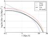 |
Fig. 1 Void size function predicted by four different models. The blue dot-dashed line represents the linear theory result given by Eq. (3). The red dashed line is the SvdW model given by Eq. (4). The black solid line is the Vdn model given by Eq. (5). The green dotted line is the void size function obtained from the Press & Schechter (1974) mass function modified with Eq. (7). |
The void size function can also be predicted directly from the halo mass function2 (see Chongchitnan & Hunt 2017, and references therein). Specifically, the probabilities that the value of the local density contrast smoothed on scale R, δR, is above or below a certain threshold δv, are related to each other by the following equation:  (6)By taking the derivative of Eq. (6)with respect to R, it results that the halo size function, that is proportional to dP(δR>δv) / dR, is equivalent to the void size function, that is proportional to dP(δR<δv) / dR. Thus, to obtain the void size function, we can use the following equation:
  (7)The last equality comes from the assumed void sphericity. Equation (7)gives the comoving number density of voids per unit effective radius in linear theory, that is analogous to Eq. (3), with the difference that it only depends on one single underdensity threshold, δv. Following the same line of reasoning used to compute Eqs. (4)and (5), it is possible to derive the void size function in the non-linear regime from the halo mass function. As an example, the green dotted line in Fig. 1 shows a volume conserving size function obtained from the Press & Schechter (1974) mass function. A detailed comparison between the implemented size function models with measured void number counts extracted from numerical simulations is provided in Ronconi et al. (in prep.).
3. The size function of cosmic voids in the distribution of biased tracers
To extract unbiased cosmological constraints from the number counts of cosmic voids detected in galaxy redshift surveys, the tracer bias has to be correctly taken into account (see e.g. Pollina et al. 2016). Indeed, voids in the DM and in the DM halo density fields do not trace the same underdensity regions. To account for the effect of tracer bias, the void size function has to be modified by changing the shell-crossing underdensity threshold with a scale- and bias-dependent barrier (Furlanetto & Piran 2006).
Even though this solution might work in principle, the analytical framework is computationally time consuming, and yields underdensity threshold values that are too low to be applied in realistic tracer samples. To overcome this issue, we implemented a simpler method to embed the bias dependency in the underdensity threshold value. Pollina et al. (2017) found that the relation between the non-linear density contrast of tracers,  , and matter,
  , around voids is linear and determined by a multiplicative constant which corresponds to the value of the bias parameter of the tracer sample, b:
  (8)To recover the linear density contrast of tracers needed to compute the void size function,
  , we apply the fitting formula provided by Bernardeau (1994) to the non-linear value given by Eq. (8), as follows:
 ![Mathematical equation: \begin{equation} \label{eq:bias02} \delta_{v,\,\text{tr}}^{\rm L} = \mathcal{C}\, \bigl[1 - (1 + b\, \delta_{v,\, \text{DM}}^{\rm NL})^{-1/\mathcal{C}} \bigr], \end{equation}](/articles/aa/full_html/2017/11/aa30852-17/aa30852-17-eq31.png) (9)with
(9)with  . Both Eq. (9) and its inverse have been implemented in the CBL, to recover the non-linear density contrast that is used to estimate the void expansion factor, r(rL). These built-in functions can be used to obtain the void size function with the models described in Sect. 2. An application of this method is presented in Ronconi et al. (in prep.).
4. Void-catalogue cleaner
4.1. The method
One of the main issues in exploiting cosmic voids as cosmological probes lies in the different void definitions adopted in observations and theoretical models. In particular, the size function models described in Sect. 2 define the cosmic voids as underdense, spherical, non-overlapped regions that have gone through shell crossing. To extract cosmological information from void distributions it is thus required either to use the same definition when detecting voids from real galaxy samples, or to clean properly the void catalogues detected with standard methods.
Following the latter approach, we expanded the CBL by implementing a new algorithm to manage a detected void catalogue to make it directly comparable to model predictions3. The algorithm is used to select and rescale the underdense regions. The procedure is completely independent of the void finding algorithm used to select the underdensities, since it only requires the void centre positions. Optionally, the user can also provide (i) the effective radii, Reff, that is, the radii of the spheres having the same volume of the considered structures; (ii) the central density of the regions, ρ0, that is, the density within a small sphere around the centres; and (iii) the density contrast between the central and the bordering regions, Δv. Alternatively, the latter two quantities are computed by two specific CBL functions4, while the former is set to a large enough value (see description below).
To implement our cleaning algorithm, we follow the procedure described in Jennings et al. (2013), which can be divided into three steps.
-
First step: we consider two selection criteria to remove non-relevant objects, that are: (i) underdensities whose effective radii are outside a given user-selected range [rmin,rmax]; if the effective radius, Reff, is not provided, it is automatically set to rmax; and (ii) underdensities that have a central density higher than
 , where
  is a given non-linear underdensity threshold, and
  is the mean density of the sample. We also included a third optional substep to deal with ZOBOV-like void catalogues. Specifically, we prune the underdensities that do not satisfy a statistical-significance criterium, Δv> Δv,0, where Δv,0 is a multiple of the typical density contrast due to Poisson fluctuations. Threshold values for several N-σ reliabilities are reported in Neyrinck (2008). The user can select which of these three sub-steps to run.
 -
Second step: we rescale the underdensities to select shell-crossing regions. To satisfy this requirement, we impose the same density threshold as the one used by theoretical models (Eq. (1)). To this end, our algorithm reconstructs the density profile of each void candidate in the catalogue, exploiting the highly optimised and parallelised chain-mesh algorithm implemented in the CBL5. After this step, the void effective radius is computed as the largest radius from the void centre which encloses an underdensity equal to δv.
-
Third step: finally, we check for overlaps. This last step is aimed to avoid double countings of cosmic voids. The collection of regions left from the previous steps are scanned one by one, checking for overlappings. When two voids do overlap, one of them is rejected. We consider two different criteria, dubbed larger-favoured and smaller-favoured. In the larger-favoured (smaller-favoured) case, one of the two overlapping voids is rejected according to which of them has the higher (lower) central density (central density selected) or the lower (higher) density contrast (density contrast selected). The user can choose which one of these criteria to apply. Also this step is optimised by exploiting the chain-mesh algorithm.
4.2. Impact of the cleaning steps
Figure 2 shows the void size distribution at the different steps of the cleaning algorithm6. The original void sample has been detected with the VIDE void finder (Sutter et al. 2015) from a ΛCDM N-body simulation with 2563 DM particles, and side length of 128 Mpc /h. The different symbols show the void size function after each step of the procedure, as indicated by the labels.
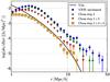 |
Fig. 2 The void size function at the different steps of the cleaning procedure. The blue dots show the distribution of voids detected by VIDE from a ΛCDM N-body simulation. The green triangles are obtained by applying both the rmin−rmax criterion and the central density criterion (first step). The red upside-down triangles show the void distribution after having rescaled the voids (second step), while the orange squares are the final output of the cleaning algorithm in case the larger-favoured overlapping criterion chosen (third step) is the decreasing central density (for the density contrast criterion see Fig. D.1). The black line shows the Vdn model prediction. |
The first selection criterion removes the voids with a radius either smaller than twice the mean particle separation, that for this simulation is 0.5 Mpc/h, or larger than half the boxside length. The effect of this first step is negligible in the size range shown in the Figure. Then the algorithm removes all the voids with central density higher than  (second selection criterion of the first cleaning step).
The VIDE void radii enclose a compensation wall, that is, an overdense region at the border of the density basin where the matter evacuated from the inner part accumulates. The second cleaning step of our algorithm provides void radii that are always smaller than the VIDE ones, thus substantially modifying the void distribution, which is shifted to smaller radii. Moreover, the total number count is decreased due to the removal of those underdensities whose radii have been shrinked to zero.
As explained in Sect. 4.1, the cleaning algorithm provides different options to deal with overlapping voids. With the smaller-favoured criterion (see Appendix D), the size distribution has a loss of power at large radii (r > Mpc /h). On the other hand, voids with radii up to tens of Mpc/h are present when the larger-favoured central density criterion (ρc) is applied.
Figure 2 shows that all the steps of our cleaning procedure are required to match the theoretical predictions. However, if we clean the overlapping voids according to their density contrast, too many large voids are erased (see Appendix D), leading to an overcleaning. Better results are found with the larger-favoured central density criterion, which provides a good match in the range 2−10 Mpc /h. The turnover at small radii appears to be in a different location after the cleaning of the void catalogue. In the uncleaned catalogue, the loss of power becomes relevant at around four times the mean inter-particle separation (≈ 2 Mpc /h). As a result of the rescaling process, small voids in the cleaned catalogue can have radii smaller than the resolution limit. This leads to a plateau in the size function at small radii.
The good agreement between the size distribution of voids in our cleaned catalogue and the Vdn model demonstrates that there is no need to fine-tune the model parameters (as has been done in previous works). A systematic comparison of different size function models is given in Ronconi et al. (in prep.), who investigate the possibility of constraining cosmological parameters from the size distribution of cosmic voids, focusing in particular on the case of biased samples.
5. Conclusions
We implemented a set of new numerical tools to analyse cosmic void catalogues and model their size distributions. The software is implemented inside the CosmoBolognaLib, a large set of open source C++/Python numerical libraries.
Even though some numerical toolkits for the detection of cosmic voids have been provided in the literature, no cosmological libraries with void-dedicated tools were available. The CBL provides a set of highly optimised methods to handle catalogues of extragalactic sources, to measure statistical quantities, such as two-point and three-point correlation functions, and to perform Bayesian statistical analyses, specifically to derive cosmological constraints. This set of libraries is a living project, constantly expanding and upgrading. The aim of this work was to upgrade the existing software by adding new numerical tools for a cosmological exploitation of cosmic void statistics.
We implemented different size function models, for voids detected in both DM and DM halo density fields. Moreover, we provide a catalogue-cleaning algorithm, that can be used to manage void samples obtained with any void finder. This point is crucial in order to offer a common ground to compare results obtained independently. A new void finder based on dynamical criteria, fully integrated in the CBL, will be released in the near future (Elyiv et al. 2015; Cannarozzo et al., in prep.).
The doxygen documentation of all the classes and methods implemented in this work is provided at the same webpage where the libraries can be downloaded, together with a set of sample codes that show how to use this software.
The models are implemented in the cosmobl::cosmology::Cosmology class.
The mass function is implemented in the cosmobl::cosmology::Cosmology class.
Specifically, we implemented a new dedicated catalogue constructor in the cosmobl::catalogue::Catalogue class.
The two functions to compute ρ0 and Δv are cosmobl::compute_centralDensity() and cosmobl::compute_densityContrast(), respectively.
The chain-mesh algorithm is implemented in the cosmobl::chainmesh class.
The size distribution has been computed with the cosmobl::catalogue::var_distr() function of the cosmobl::catalogue::Catalogue class.
We used a similar code to obtain the model size distributions shown in Fig. 1.
We used a similar code to obtain the size distributions shown by coloured points in Fig. 2.
The provided input catalogue has been obtained with VIDE from a 128 Mpc side length ΛCDM N-body simulation, with 2563 DM particles.
Acknowledgments
We thank C. Cannarozzo, L. Moscardini, M. Baldi and A. Veropalumbo for useful discussions about numerical and scientific issues related to these libraries. We also thank M. Baldi for providing the N-body simulations used in this work. We want to thank the anonymous referee for the useful suggestions that helped to improve this paper.
References
- Barreira, A., Cautun, M., Li, B., Baugh, C. M., & Pascoli, S. 2015, JCAP, 08, 028 [CrossRef] [Google Scholar]
- Bernardeau, F. 1994, ApJ, 427, 51 [NASA ADS] [CrossRef] [Google Scholar]
- Blumenthal, G. R., da Costa, L. N., Goldwirth, D. S., Lecar, M., & Piran, T. 1992, ApJ, 388, 234 [CrossRef] [Google Scholar]
- Bond, J. R., Cole, S., Efstathiou, G., & Kaiser, N. 1991, ApJ, 379, 440 [NASA ADS] [CrossRef] [Google Scholar]
- Cai, Y.-C., Padilla, N., & Li, B. 2015, MNRAS, 451, 1036 [NASA ADS] [CrossRef] [Google Scholar]
- Chongchitnan, S., & Hunt, M. 2017, JCAP, 03, 049 [NASA ADS] [CrossRef] [Google Scholar]
- Clampitt, J., Cai, Y.-C., & Li, B. 2013, MNRAS, 431, 749 [NASA ADS] [CrossRef] [Google Scholar]
- Colberg, J. M., Sheth, R. K., Diaferio, A., Gao, L., & Yoshida, N. 2005, MNRAS, 360, 216 [NASA ADS] [CrossRef] [Google Scholar]
- Colberg, J. M., Pearce, F., Foster, C., et al. 2008, MNRAS, 387, 933 [NASA ADS] [CrossRef] [Google Scholar]
- Elyiv, A., Marulli, F., Pollina, G., et al. 2015, MNRAS, 448, 642 [NASA ADS] [CrossRef] [Google Scholar]
- Furlanetto, S. R., & Piran, T. 2006, MNRAS, 366, 467 [NASA ADS] [CrossRef] [Google Scholar]
- Hawken, A. J., Granett, B. R., Iovino, A., et al. 2017, A&A, in press, DOI: 10.1051/0004-6361/201629678 [Google Scholar]
- Jennings, E., Li, Y., & Hu, W. 2013, MNRAS, 434, 2167 [NASA ADS] [CrossRef] [Google Scholar]
- Lacey, C., & Cole, S. 1993, MNRAS, 262, 627 [NASA ADS] [CrossRef] [Google Scholar]
- Lacey, C., & Cole, S. 1994, MNRAS, 271, 676 [Google Scholar]
- Lam, T. Y., Clampitt, J., Cai, Y.-C., & Li, B. 2015, MNRAS, 450, 3319 [NASA ADS] [CrossRef] [Google Scholar]
- Li, B., Zhao, G.-B., & Koyama, K. 2012, MNRAS, 421, 3481 [NASA ADS] [CrossRef] [Google Scholar]
- Marulli, F., Veropalumbo, A., & Moresco, M. 2016, Astronomy and Computing, 14, 35 [NASA ADS] [CrossRef] [Google Scholar]
- Massara, E., Villaescusa-Navarro, F., Viel, M., & Sutter, P. M. 2015, JCAP, 11, 018 [NASA ADS] [CrossRef] [Google Scholar]
- Nadathur, S., & Hotchkiss, S. 2015, MNRAS, 454, 2228 [NASA ADS] [CrossRef] [Google Scholar]
- Neyrinck, M. C. 2008, MNRAS, 386, 2101 [NASA ADS] [CrossRef] [Google Scholar]
- Pisani, A., Sutter, P. M., Hamaus, N., et al. 2015, Phys. Rev. D, 92, 083531 [NASA ADS] [CrossRef] [Google Scholar]
- Pollina, G., Baldi, M., Marulli, F., & Moscardini, L. 2016, MNRAS, 455, 3075 [NASA ADS] [CrossRef] [Google Scholar]
- Pollina, G., Hamaus, N., Dolag, K., et al. 2017, MNRAS, 469, 787 [NASA ADS] [CrossRef] [Google Scholar]
- Press, W. H., & Schechter, P. 1974, ApJ, 187, 425 [NASA ADS] [CrossRef] [Google Scholar]
- Sahlén, M., & Silk, J. 2016, ArXiv e-prints [arXiv:1612.06595] [Google Scholar]
- Sahlén, M., Zubeldía, Í., & Silk, J. 2016, ApJ, 820, L7 [NASA ADS] [CrossRef] [Google Scholar]
- Sheth, R. K., & van de Weygaert, R. 2004, MNRAS, 350, 517 [NASA ADS] [CrossRef] [Google Scholar]
- Springel, V. 2005, MNRAS, 364, 1105 [NASA ADS] [CrossRef] [Google Scholar]
- Sutter, P. M., Lavaux, G., Wandelt, B. D., & Weinberg, D. H. 2012, ApJ, 761, 44 [NASA ADS] [CrossRef] [Google Scholar]
- Sutter, P. M., Lavaux, G., Hamaus, N., et al. 2015, Astronomy and Computing, 9, 1 [Google Scholar]
- Viel, M., Colberg, J. M., & Kim, T.-S. 2008, MNRAS, 386, 1285 [NASA ADS] [CrossRef] [Google Scholar]
- Zentner, A. R. 2007, Int. J. Mod. Phys. D, 16, 763 [NASA ADS] [CrossRef] [Google Scholar]
- Zivick, P., Sutter, P. M., Wandelt, B. D., Li, B., & Lam, T. Y. 2015, MNRAS, 451, 4215 [NASA ADS] [CrossRef] [Google Scholar]
Appendix A: Size function example
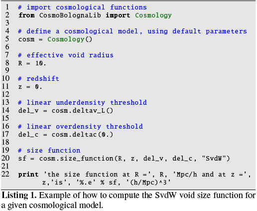
The following Python code illustrates how to compute the theoretical size function of cosmic voids for a given cosmological model7. This is done by creating an object of the Cosmology class and then using one of its internal functions to compute the size function. Alternatively to what is shown in this example, the free model parameters can be set via a parameter file managed by a dedicated class (i.e. cosmobl::ReadParameters), as shown in the CBL webpage.
Appendix B: Void-catalogue-cleaning example
The following C++ code shows how to construct a catalogue of spherical non-overlapped voids which have gone through shell-crossing, and how to store it in an ASCII file8.
In step I, an ASCII void catalogue9 is read by the constructor, searching for columns containing the requested attributes. In step II, we load the original N-body simulation snapshot into a halo catalogue. Optionally, the user can exploit a constructor specifically designed to read binary output files obtained with GADGET-2 (Springel 2005). Then we compute the snapshot properties (i.e. volume and mean particle separation), and use them to store the DM particle positions in a chain-mesh. In step III, after computing the central densities of voids in the input catalogue, we call the catalogue constructor which implements the algorithm described in Sect. 4. Finally, we use a built-in function of the CBL to store the new catalogue in an ASCII file.

We release also a fully automatic Python pipeline that performs all the cleaning steps of the method. It is available with the latest CosmoBolognaLib release. By setting a self-explaining parameter file, also provided in the package, the user can control each variable of the code. Both the Python script, called cleanVoidCatalogue.py, and the parameter file can be found in the Examples folder of the CosmoBolognaLib package.
Appendix C: Time performances of the cleaning algorithm
We test the time performances of the presented cleaning algorithm as a function of both the density and volume of the input catalogue. The analysis has been performed on one single cluster node with 2 GHz of clock frequency and 64 Gb of RAM memory.
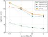 |
Fig. C.1 Time performances of the cleaning algorithm as a function of the mean inter-particle separation. The orange dots show the total amount of time spent by the code, while the other symbols refer to each step of the cleaning method, as indicated by the labels. |
Figure C.1 shows the computational time as a function of resolution, that is measured in terms of the mean inter-particle separation (m.i.s.). Both the time spent by each single step of the procedure and the global time are shown. The volume of the simulation used for this analysis is fixed at V = 1283(Mpc/h)3. The first step of the cleaning method is the least time-consuming, while the other two have a similar impact: while the second step contributes the most to the total time at low resolution (high m.i.s.), it becomes less relevant with respect to the third step at higher resolution (small m.i.s.). The total amount of time spent by the algorithm, as well as that spent by each single step, increases almost exponentially with increasing resolution.
A similar behaviour is found as a function of volume. The performances of the algorithm at fixed resolution (m.i.s. = 2 Mpc/h) and with varying total volume are shown in Fig. C.2.
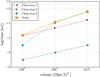 |
Fig. C.2 The same of Fig. C.1, but as a function of volume. The resolution is fixed at m.i.s. = 2 Mpc/h. |
As in the fixed volume case, the first step is the least time-consuming. The third step is less time-consuming at small volumes than the second step, and it takes more time at larger volumes.
The outlined behaviour shows that the time spent by the algorithm increases exponentially with increasing number of voids. In the first case (Fig. C.1), a larger number of voids are detected at small radii when the resolution is increased, while in the second case (Fig. C.2) more voids are found at all radii when increasing the volume.
Appendix D: Testing how to clean the overlapping voids
The algorithm presented in this work provides two possible methods to clean the overlapping voids. The choice depends on the purpose of the study the user wants to perform. Figure D.1 compares the void size function obtained with all the implemented criteria.
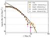 |
Fig. D.1 Comparison between the void size functions obtained with the smaller-favoured (central density criteria – yellow diamonds; density contrast criteria – grey pentagons) and the larger-favoured density contrast overlapping criteria (central density criteria – orange squares; density contrast criteria – magenta stars) of the third step of the cleaning method. The black line shows the Vdn model prediction. |
The void size functions obtained with all these different criteria agree reasonably well with the Vdn model. The two smaller-favoured criteria select deeper density basins, that typically correspond to smaller voids. Such a choice is not convenient for cosmological analyses that aim to extract constraints from the void size function in the largest possible range of radii. Nevertheless, it can be a convenient choice if the goal is to study small voids around the resolution limit of the sample.
All Figures
|
Fig. 1 Void size function predicted by four different models. The blue dot-dashed line represents the linear theory result given by Eq. (3). The red dashed line is the SvdW model given by Eq. (4). The black solid line is the Vdn model given by Eq. (5). The green dotted line is the void size function obtained from the Press & Schechter (1974) mass function modified with Eq. (7). |
| In the text | |
|
Fig. 2 The void size function at the different steps of the cleaning procedure. The blue dots show the distribution of voids detected by VIDE from a ΛCDM N-body simulation. The green triangles are obtained by applying both the rmin−rmax criterion and the central density criterion (first step). The red upside-down triangles show the void distribution after having rescaled the voids (second step), while the orange squares are the final output of the cleaning algorithm in case the larger-favoured overlapping criterion chosen (third step) is the decreasing central density (for the density contrast criterion see Fig. D.1). The black line shows the Vdn model prediction. |
| In the text | |
|
Fig. C.1 Time performances of the cleaning algorithm as a function of the mean inter-particle separation. The orange dots show the total amount of time spent by the code, while the other symbols refer to each step of the cleaning method, as indicated by the labels. |
| In the text | |
|
Fig. C.2 The same of Fig. C.1, but as a function of volume. The resolution is fixed at m.i.s. = 2 Mpc/h. |
| In the text | |
|
Fig. D.1 Comparison between the void size functions obtained with the smaller-favoured (central density criteria – yellow diamonds; density contrast criteria – grey pentagons) and the larger-favoured density contrast overlapping criteria (central density criteria – orange squares; density contrast criteria – magenta stars) of the third step of the cleaning method. The black line shows the Vdn model prediction. |
| In the text | |
Current usage metrics show cumulative count of Article Views (full-text article views including HTML views, PDF and ePub downloads, according to the available data) and Abstracts Views on Vision4Press platform.
Data correspond to usage on the plateform after 2015. The current usage metrics is available 48-96 hours after online publication and is updated daily on week days.
Initial download of the metrics may take a while.