| Issue |
A&A
Volume 606, October 2017
|
|
|---|---|---|
| Article Number | A143 | |
| Number of page(s) | 6 | |
| Section | Celestial mechanics and astrometry | |
| DOI | https://doi.org/10.1051/0004-6361/201731681 | |
| Published online | 26 October 2017 | |
Tropospheric delay modelling and the celestial reference frame at radio wavelengths
Department of Geodesy and GeoinformationTechnische Universität Wien, Karlsplatz 13, 1040 Vienna, Austria
e-mail: david.mayer@tuwien.ac.at
Received: 31 July 2017
Accepted: 29 August 2017
Aims. We examine the relationship between Very Long Baseline Interferometry (VLBI) tropospheric delay modelling and source positions. In particular, the effect of a priori ray-traced slant delays on source declination is investigated.
Methods. We estimated source coordinates as global positions from 5830 geodetic VLBI sessions incorporating about 10 million group delay measurements. This data set was used for the International Celestial Reference Frame 3 (ICRF3) prototype solutions as of December 2016.
Results. We report on a significant bias in source declination of about 50 μas, which can be found between a normal solution and a solution where a priori ray-traced slant delays are used. More traditional tropospheric delay modelling techniques, such as a priori gradients, are tested as well. Significant differences of about 30 μas in declination can only be found when absolute constraints are used for a priori gradient models. Further, we find that none of these models decrease the declination bias between ICRF3 prototype solutions and ICRF2.
Key words: atmospheric effects / astrometry / reference systems
© ESO, 2017
 Open Access article, published by EDP Sciences, under the terms of the Creative Commons Attribution License (http://creativecommons.org/licenses/by/4.0),
which permits unrestricted use, distribution, and reproduction in any medium, provided the original work is properly cited.
Open Access article, published by EDP Sciences, under the terms of the Creative Commons Attribution License (http://creativecommons.org/licenses/by/4.0),
which permits unrestricted use, distribution, and reproduction in any medium, provided the original work is properly cited.
1. Introduction
The current realisation of the International Celestial Reference System (ICRS), the International Celestial Reference Frame 2 (ICRF2) (Ma et al. 2009; Fey et al. 2015), replacing the previous solution ICRF1 (Ma et al. 1998), was established 2009. The ICRF2 used the Very Long Baseline Interferometry (VLBI) group delay data from 1979 until March 2009. Since the release of the ICRF2 the amount of observed group delay measurements has almost doubled from 6.5 million group delays in 2009 to 10.5 million group delays in 2016. The increased amount of data and the higher demands on accuracy, with the Gaia mission providing a reference frame with comparable accuracy (Mignard et al. 2016; Petrov & Kovalev 2017), has motivated the geodetic VLBI community to release an updated reference frame in 2018. This will be called ICRF3.
The handling (modelling and estimating) of the tropospheric delays is the limiting factor in terms of accuracy in the current geodetic VLBI processing; see Pany et al. (2011) and Petrachenko et al. (2009). There has been steady progress in recent years with several new tropospheric delay modelling techniques emerging. In particular, ray tracing, which uses weather models to estimate slant path delays through the troposphere, is an interesting new approach to modelling the troposphere. Two groups tested ray-traced delays in geodetic VLBI analysis (Eriksson et al. 2014; Hofmeister & Böhm 2017) and identified this approach as an interesting alternative to the standard approach of estimating gradients when station coordinates are considered. However, the influence of ray tracing on source positions is not discussed in either of these two publications. Furthermore, new gradient models were developed by Landskron et al. (2015) and are shown to improve station positions; however, source positions have not yet been considered.
These new developments and the increased demand on source position accuracy motivated us to test these new tropospheric delay models and question the state-of-the-art tropospheric delay modelling techniques.
2. Data and analysis
In order to evaluate the effect of tropospheric delay modelling on source positions, celestial reference frames are estimated and used for comparison.
2.1. Naming convention
A naming convention is chosen for the different CRF solutions that helps to identify the various solutions with a single glance. These names are as short as possible and carry meaning about the data set and parameterisation. The convention is as follows:
-
the first section resembles the data set. It can either be Vie16 (thedata range for ICRF3) or Vie09 (the data range for ICRF2).
-
The second section relates to the troposphere delay parameterisation. It can be DAO (a priori DAO gradients), GRD (a priori GRAD gradients), RAY (a priori ray-traced delays) or ELW (elevation angle dependent weighting). More information concerning the parameterisation can be found in the corresponding sections.
-
The last entry can either be fixgd (fix gradients) or estgd (estimate gradients).
For example, the Vie09-RAY-fixgd reference frame covers the data range of the ICRF2 (1979 – March 2009) with a priori ray-traced delays and fixed, i.e. no estimation of gradients.
2.2. The Vienna ICRF3 prototype solution (Vie16)
The Vienna VLBI group at the Technische Universität Wien, Vienna, Austria is contributing to the development of the new celestial reference frame by estimating a version of the ICRF3 using an independent analysis software called VieVS (Vienna VLBI and Satellite Software; Böhm et al. 2012). This version is used as a basis for further comparisons.
The general data analysis for geodetic VLBI is basically divided into two steps when a reference frame is estimated. The first step is a single session analysis with one normal equation matrix per session as a result. In a second step the global parameters are estimated. Basically, all the normal equations are rearranged and divided into matrices containing the session specific (arc parameters – rapidly changing with time) parameters, such as tropospheric parameters, clock parameters and Earth orientation parameters (EOP), and common parameters (global parameters – not changing with time), such as station coordinates and source coordinates. The reduced normal equation matrices, those containing the global parameters, are then stacked to produce one global normal equation system. The parameters of interest, in our case the source and station positions, can be estimated using least squares adjustment.
A priori geophysical models used in the present analysis generally follow the IERS Conventions 2010 by Petit & Luzum (2010) with the addition of the antenna thermal deformation model by Nothnagel (2009) and the tidal/non-tidal atmospheric loading (APLO) model by Wijaya et al. (2013). Nutation and precession are modelled using the IAU 2000A and IAU 2006 model, respectively, as suggested in the electronic updates of the IERS Conventions by Petit & Luzum (2010).
Formal errors from the correlator are usually too optimistic, which is why these errors are increased by 1 cm2.
The following single session parameterisation is used for generating the normal equations per session:
-
clocks at the stations are estimated as a quadratic polynomial forlong-term variations and piecewise linear offsets (PWLO) every60 min with relative constraints of1.3 cm for short-term variations.
-
Troposphere wet zenith delays are estimated as PWLO per station every 30 min with relative constraints of 1.5 cm.
-
Tropospheric gradients in north-south and east-west direction are estimated per station as PWLO every 6 h with relative constraints of 0.5 mm.
-
Earth orientation parameters are estimated as one offset per session (realised as PWLO every 48 h with very tight constraints).
-
Estimation of station coordinates that only observe in a limited number (not enough sessions to estimate a reliable velocity) of sessions (less than 20 sessions or a time span of less than 2 yr).
-
Estimation of source coordinates that experience systematic variation in their time series (so-called special handling sources).
The following parameterisation is used for setting up the global solution:
-
station coordinates and velocities for the reference epoch 2005are estimated using no-net-rotation and no-net-translationconstraints on 22 stations to align the terrestrial reference frame tothe ITRF2014 (Altamimi et al. 2016).
-
Discontinuities are introduced to stations that experienced a jump in their coordinates – either through seismic events or humanly introduced. If the discontinuity happened without any recorded seismic event (e.g. relocation or repair of the telescope) the velocity is constrained to be the same before and after the event.
-
Post seismic deformation is modelled by the ITRF2014. Additional artificial discontinuities are introduced at selected sites when necessary.
-
Stations on the same site are constrained to have the same velocity.
-
Source coordinates are estimated for all sources with more than three observations; sources with fewer than four observations are excluded in the single session step. No-net-rotation constraints are imposed on 295 sources (defining sources of the ICRF2) to align the celestial reference frame with the ICRF2.
This set of parameters is set as default for every reference frame presented in this paper, if not specified otherwise.
2.3. Ray-traced delays
In geodetic VLBI the troposphere delays are usually estimated. The standard processing includes the estimation of wet zenith delays (ZWD) in a certain time interval while the zenith hydrostatic delays are modelled a priori with pressure values at the site (Saastamoinen 1972). These zenith delays are mapped to lower elevation angles using a mapping function. The most accurate mapping functions currently available are derived from numerical weather models; see Böhm et al. (2006). To account for the asymmetry of the troposphere, north-south and east-west gradients are usually estimated at a certain time interval.
In contrast, ray tracing uses a priori information from numerical weather models to estimate the path and the corresponding delay through the troposphere for every observation. This calculated path delay can then be used to correct the actual VLBI observation.
A combination of traditional tropospheric delay modelling and ray-traced delays usually provides the best results, e.g. ray-traced delays used a priori and gradients estimated (Hofmeister & Böhm 2017).
A priori ray-traced tropospheric slant delays used in our analysis are calculated using the program RADIATE, by Hofmeister (2016), which was developed at the Department of Geodesy and Geoinformation at the Technische Universität Wien, Vienna, Austria. This program uses operational and re-analysed weather data from the European Centre for Medium-Range Weather Forecasts (ECMWF) with a spatial resolution of one degree and a temporal resolution of six hours to determine an a priori tropospheric delay per observation.
2.4. A priori gradients
2.4.1. Mean site gradients computed from GSFC Data Assimilation Office (DAO)
In the Vienna ICRF3 prototype solution gradients are estimated (no a priori gradients are used) every 6 h with relative constraints. Another option would be to use a priori gradients, such as the DAO model by MacMillan (1995) and MacMillan & Ma (1997). These constant gradients are calculated from numerical weather models and, in addition to station dependent systematic effects, account for the systematic north-south gradients.
2.4.2. GRAD gradients
A more refined gradient model, the so-called GRAD model, by Landskron et al. (2015), which estimates a time series of a priori gradients from numerical weather models, was developed at the Department of Geodesy and Geoinformation at the Technische Universität Wien, Vienna, Austria. This model provides gradients with a 6 h time resolution and is based on ray-traced delays estimated with the program RADIATE.
2.5. Elevation dependent weighting
In order to decorrelate the station height, troposphere delays, and clock parameters, geodetic VLBI observes down to an elevation angle of 5o (this is the usual threshold for geodetic sessions). At such low elevation angles the influence of the troposphere is magnified and possible mismodelling has a greater effect on the solution. Therefore, if we introduce an elevation angle dependent noise factor instead of the constant value, thereby effectively downweighting observations with low elevation angle, we expect an effect on source declination. The amount of added noise n (in pico seconds) was calculated with Eq. (1), where e1 and e2 are the elevation angles of the two stations participating in the observation, i.e. 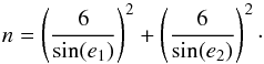 (1)
(1)
3. Method
3.1. Source coordinate difference
Since we are interested in the effect of different tropospheric delay models on the ICRF we compare the resulting source coordinates. In order to keep the plots simple we decided to focus on a subset of sources, the so-called defining sources. These sources define the orientation of the ICRF2. Only the most stable sources with the most observations were selected as defining sources. However, the global distribution of the sources had to be considered as well. Consequently, since the Southern Hemisphere has less VLBI telescopes than the northern hemisphere, southern sources are not as precise as northern sources.
In order to compare the difference of many models with one glance we decided to approximate their coordinates with a moving average filter with a window size of 30 sources. An illustration of this is depicted in Fig. 1 where the underlying data (declination difference – blue dots) is approximated with a moving average filter (black line). However, the differences of particularly interesting models are then illustrated and discussed separately without any approximation.
3.2. Declination bias
When comparing Vie16 to Vie09 (same data as ICRF2) one finds a systematic difference in declination, this is the so-called declination bias. A depiction of this bias can be found in Fig. 1 where the difference in declination is plotted with respect to declination. Only the 295 defining sources are shown. A very similar systematic difference was found by other groups using independent analysis with different software (personal communication with the IAU Working Group on the ICRF3). The reason for this shift in declination is not yet fully understood. Basically two scenarios are possible. First, the ICRF2 was estimated from a data set that was dominated by observations by northern stations. Therefore, southern sources are mainly observed under low elevation angle from northern stations, which in turn systematically adds up tropospheric delay modelling errors. The ICRF3 data set includes many new observations from southern stations (in particular the AuScope array should be mentioned here; see Plank et al. 2016, for more detail) and, therefore, many observations to southern sources at high elevation angles. These new observations would expose present systematic effects and these would show up as a bias in declination. The second argument is that the new observations from the southern stations have shortcomings (some sort of systematic station dependent effect). This is a reasonable possibility since the previously mentioned AuScope array, which is responsible for a majority of the new observations to southern sources, consists of three identically constructed low-cost antennas. Interestingly, observations with the station HOBART12 are responsible for a majority of the bias; see Mayer et al. (2017).
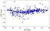 |
Fig. 1 Declination bias between Vie16 and Vie09 (Vie16 minus Vie09). Only ICRF2 defining sources are depicted. |
Tropospheric delay modelling has a potential effect on this bias that we see in declination. Since understanding this relationship is of utmost importance for the reference frame community and the release of the ICRF3, we discuss the effect of these models on the declination bias in detail below.
4. Results
4.1. Source coordinate difference
In this section we focus on the influence of tropospheric delay modelling on the source coordinates.
Figure 2 depicts the difference, i.e. the ICRF3 prototype solution with normal parameterisation minus solution with respective model, in declination (upper plot, ΔDE) and right ascension (lower plot, ΔRA·cos(DE)) of the ICRF2 defining sources of the various solutions. A clear systematic difference in declination for the solutions where ray-traced delays are used is visible. The declination of sources from solutions with a priori gradients (DAO and GRAD) and absolute constraints seems to be systematically offset as well. Elevation dependent weighting influences the source declination with changes of about 10 μas.
The right ascension of all solutions agrees within 20 μs with the reference solution.
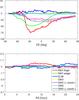 |
Fig. 2 Differences in declination (upper plot) and right ascension (lower plot) of the ICRF2 defining sources. Solution with normal parameterisation minus respective model solution. The legend is the same for both. For readability reasons the naming convention in the legend is abbreviated (only the suffix that specifies the model used is kept). |
4.2. Declination bias
In this section we discuss the influence of the choice of tropospheric delay modelling on the declination bias, i.e. we always use the same approach for tropospheric delay modelling but change the time span.
Figure 3 illustrates the declination biases from solutions with different models. We plot the differences in source declination (ΔDE) of a solution using the ICRF3 data set minus a solution using the ICRF2 data set. The same model was always used for both data sets.
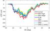 |
Fig. 3 Differences in declination of the ICRF2 defining sources. Solution with ICRF3 data set minus solution with ICRF2 data set. The same model is used in both data sets. For readability reasons the naming convention in the legend is abbreviated (only the suffix that specifies the model used is kept). |
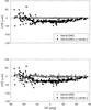 |
Fig. 4 Differences in declination of the ICRF2 defining sources (all 295 sources are depicted). The upper plot depicts the solution with normal parameterisation minus solutions with a priori DAO gradients. The lower plot is similar with the difference that the GRAD model was used. |
The declination bias in our reference solution is depicted in black and it is almost identical with the declination bias of the solution where DAO gradients are used a priori (yellow). No solution decreases the declination bias. However, we can clearly see a systematic difference when ray-traced delays are used.
5. Discussion
5.1. Source coordinate difference
When considering Fig. 2 we can assume that using a priori gradient models, such as the DAO and GRAD models, does not have a big impact on source coordinates. However, when we put absolute constraints on these models, as is done in the current ICRF2 solution, we find a significant deviation in declination. A detailed depiction of this effect is provided in Fig. 4 where the difference between the reference solution and the solution with a priori gradients (for the DAO and GRAD models) for all ICRF2 defining sources is plotted. Putting absolute constraints (0.5 mm) on these a priori gradients affect the sources in mid-declinations most. The effect is larger when the GRAD model is used. Sources in this region have many observations through the atmospheric bulge around the equator. The DAO and GRAD models account for this effect, which is why we can see the biggest influence here. This feature demonstrates that systematic effects in the gradients cannot be properly accounted for by VLBI observations, at least not at sites with sparse observation density on the sky. Especially, sessions in the early VLBI history suffer from this effect, which results in unrealistic gradient estimates for these sessions. Using absolute constraints mitigates this effect; see Spicakova et al. (2011). Therefore, we believe that the solutions using absolute constraints on a priori gradients are more trustworthy than solutions where gradients are not constrained.
An interesting effect can be observed when ray-traced delays are used as a priori information. Figure 5, where the difference of the reference solution and the solutions with ray-traced delays is depicted, illustrates this in detail; this is shown once with gradients estimated and once with gradients fixed, i.e. without estimating gradients. Similar to Fig. 4 the ICRF2 defining sources are depicted. A clear systematic effect is visible in both solutions. When gradients are estimated (black dots) we can see a very clear systematic effect. The sources from 30o to 90o are not affected. Sources to the south are affected more with a peak at about − 30o and an interesting feature (intermediate peak) at − 60o. When gradients are not estimated (grey dots) there is a similar effect with a larger scatter.
The origin of this bias is still unclear. One possible explanation is that the traditional troposphere estimation process used in geodetic VLBI is not sufficient and accurate enough and does not absorb the whole signal owing to troposphere. Another possibility is that the ray-tracing algorithm or the underlying weather model has shortcomings; however, we have not found any evidence for that reason.
Interestingly, the source declination of Vie16-RAY-fixgd, Vie16-DAO and Vie16-GRD, which both have absolute constraints, is very similar above 30o of declination.
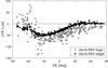 |
Fig. 5 Differences in declination of the ICRF2 defining sources (all 295 sources are depicted). Solution with normal parameterisation minus solutions with a priori ray-traced delays. |
5.2. Declination bias
When looking at Fig. 3, it is evident that they differ significantly. In particular, the solutions with ray-traced delays have a significant offset. Since the declination bias represents the difference between the old (ICRF2) and new (ICRF3) data set, we can conclude that these models affect the old and new data set differently.
One way of explaining this is that the new data (added after the release of the ICRF2) has more observations in the south, which means that the ICRF3 has less errors due to tropospheric delay mismodelling at low elevation angles. Therefore, solutions with modelling approaches that are more sensitive to tropospheric delay errors have a higher declination difference between the old and new data set.
Another possible explanation, at least for the solution without gradient estimation and the solutions with absolute constraints on gradients, is that the early sessions suffer from sparse observation density on the sky, which results in unrealistic gradient estimates. Since the ICRF3 data set includes more recent sessions than the ICRF2 data set, these early sessions do not have as much weight as in the ICRF2, which could result in a difference in declination.
However, the conclusion we can draw from Fig. 3 is that none of the models succeed in reducing the declination bias, which indicates that the declination bias is not due to tropospheric delay modelling errors.
6. Conclusions and outlook
We used the ICRF3 data set to investigate the influence of tropospheric delay modelling on source positions. A priori models for gradients, such as the DAO and the GRAD model, as well as a priori ray-traced slant delay models are tested. Further, we looked at the influence of elevation dependent weighting.
When gradient models are used a priori and gradients are estimated we find almost no effect on source position. This changes when absolute constraints are used for these gradients, which causes differences of about 30 μas in source declination.
When a priori ray-traced slant delays are used in the processing we find a significant bias in source declination of distinct shape and a maximum of about 50 μas. This reported bias does not explain the so-called declination bias.
Additionally, we discussed the impact of these models on the declination bias, which basically reflects the difference between solutions with the VLBI data set until 2009 and the VLBI data set until 2016. We find no decrease of the declination bias when any of these models are used. This indicates that the declination bias is not caused by insufficient tropospheric delay modelling but rather by a station dependent effect.
In the future we plan to compare our solutions to celestial reference frames from different wavelengths, such as K band and Ka band, or Gaia. Furthermore, we will try to implement more sophisticated stochastic models and test their influence on tropospheric delay modelling.
Acknowledgments
D.M., J.B. and H.K. are grateful to the Austrian Science Fund (FWF), which funded part of this research with the project SORTS (I2204), Radiate VLBI (P25320) and Galactic VLBI (T697-N29). We would like to thank the Vienna Scientific Cluster (VSC-3) for supporting our VLBI work. This research made use of the data provided by the IVS (Nothnagel et al. 2015).
References
- Altamimi, Z., Rebischung, P., Métivier, L., & Collilieux, X. 2016, J. Geophys. Res., 121, 6109 [Google Scholar]
- Böhm, J., Werl, B., & Schuh, H. 2006, J. Geophys. Res., 111, b02406 [Google Scholar]
- Böhm, J., Böhm, S., Nilsson, T., et al. 2012, The New Vienna VLBI Software VieVS, eds. S. Kenyon, M. C. Pacino, & U. Marti (Berlin, Heidelberg: Springer), 1007 [Google Scholar]
- Eriksson, D., MacMillan, D. S., & Gipson, J. M. 2014, J. Geophys. Res., 119, 9156 [NASA ADS] [CrossRef] [Google Scholar]
- Fey, A. L., Gordon, D., Jacobs, C. S., et al. 2015, AJ, 150, 58 [NASA ADS] [CrossRef] [Google Scholar]
- Hofmeister, A. 2016, Ph.D. Thesis, Department f. Geodäsie u. Geoinformation/ Höhere Geodäsie [Google Scholar]
- Hofmeister, A., & Böhm, J. 2017, J. Geodesy Berlin, 91, 945 [NASA ADS] [CrossRef] [Google Scholar]
- Landskron, D., Hofmeister, A., & Böhm, J. 2015, Refined Tropospheric Delay Models for CONT11 (Berlin, Heidelberg: Springer), 1 [Google Scholar]
- Ma, C., Arias, E. F., Eubanks, T. M., et al. 1998, AJ, 116, 516 [NASA ADS] [CrossRef] [Google Scholar]
- Ma, C., Arias, E. F., Bianco, G., et al. 2009, IERS Technical Note, 35 [Google Scholar]
- MacMillan, D. S. 1995, Geophys. Res. Lett., 22, 1041 [NASA ADS] [CrossRef] [Google Scholar]
- MacMillan, D. S., & Ma, C. 1997, Geophys. Res. Lett., 24, 453 [NASA ADS] [CrossRef] [Google Scholar]
- Mayer, D., Böhm, J., Krásná, H., & McCallum, L. 2017, in Proc. of the 23rd European VLBI Group for Geodesy and Astrometry Working Meeting, 15–19 May 2017 [Google Scholar]
- Mignard, F., Klioner, S., Lindegren, L., et al. 2016, A&A, 595, A5 [NASA ADS] [CrossRef] [EDP Sciences] [Google Scholar]
- Nothnagel, A. 2009, J. Geodesy Berlin, 83, 787 [Google Scholar]
- Nothnagel, A., Alef, W., Amagai, J., et al. 2015, in GFZ Data Services, Helmoltz Centre, Potsdam, Germany [Google Scholar]
- Pany, A., Böhm, J., MacMillan, D., et al. 2011, J. Geodesy Berlin, 85, 39 [NASA ADS] [CrossRef] [Google Scholar]
- Petit, G., & Luzum, B., eds. 2010, IERS Conventions 2010 (Frankfurt am Main: Verlag des Bundesamts für Kartographie und Geodäsie), IERS Technical Note, 36 [Google Scholar]
- Petrachenko, B., Niell, A., Behrend, D., et al. 2009, Design Aspects of the VLBI2010 System, Progress Report of the IVS VLBI2010 Committee, nASA/TM-2009-214180, 2009 [Google Scholar]
- Petrov, L., & Kovalev, Y. Y. 2017, MNRAS, 467, L71 [NASA ADS] [Google Scholar]
- Plank, L., Lovell, J. E. J., McCallum, J. N., et al. 2016, J. Geodesy Berlin, 1 [Google Scholar]
- Saastamoinen, J. 1972, Bull. Géod., 105, 279 [Google Scholar]
- Spicakova, H., Plank, L., Nilsson, T., Böhm, J., & Schuh, H. 2011, in 20th Meeting of the European VLBI Group for Geodesy and Astronomy, March 29-30, eds. W. Alef, S. Bernhart, & A. Nothnagel, 118 [Google Scholar]
- Wijaya, D., Böhm, J., Karbon, M., Krásná, H., & Schuh, H. 2013, Atmospheric Pressure Loading, eds. J. Böhm, & H. Schuh (Berlin, Heidelberg: Springer), 137 [Google Scholar]
All Figures
|
Fig. 1 Declination bias between Vie16 and Vie09 (Vie16 minus Vie09). Only ICRF2 defining sources are depicted. |
| In the text | |
|
Fig. 2 Differences in declination (upper plot) and right ascension (lower plot) of the ICRF2 defining sources. Solution with normal parameterisation minus respective model solution. The legend is the same for both. For readability reasons the naming convention in the legend is abbreviated (only the suffix that specifies the model used is kept). |
| In the text | |
|
Fig. 3 Differences in declination of the ICRF2 defining sources. Solution with ICRF3 data set minus solution with ICRF2 data set. The same model is used in both data sets. For readability reasons the naming convention in the legend is abbreviated (only the suffix that specifies the model used is kept). |
| In the text | |
|
Fig. 4 Differences in declination of the ICRF2 defining sources (all 295 sources are depicted). The upper plot depicts the solution with normal parameterisation minus solutions with a priori DAO gradients. The lower plot is similar with the difference that the GRAD model was used. |
| In the text | |
|
Fig. 5 Differences in declination of the ICRF2 defining sources (all 295 sources are depicted). Solution with normal parameterisation minus solutions with a priori ray-traced delays. |
| In the text | |
Current usage metrics show cumulative count of Article Views (full-text article views including HTML views, PDF and ePub downloads, according to the available data) and Abstracts Views on Vision4Press platform.
Data correspond to usage on the plateform after 2015. The current usage metrics is available 48-96 hours after online publication and is updated daily on week days.
Initial download of the metrics may take a while.