| Issue |
A&A
Volume 606, October 2017
|
|
|---|---|---|
| Article Number | A91 | |
| Number of page(s) | 13 | |
| Section | Stellar atmospheres | |
| DOI | https://doi.org/10.1051/0004-6361/201731291 | |
| Published online | 17 October 2017 | |
A combined HST and XMM-Newton campaign for the magnetic O9.7 V star HD 54879
Constraining the weak-wind problem of massive stars⋆
1 Institute for physics and astronomy, University of Potsdam, Karl-Liebknecht-Str. 24/25, 14476 Potsdam, Germany
e-mail: This email address is being protected from spambots. You need JavaScript enabled to view it.
2 Leibniz-Institute for astrophysics Potsdam (AIP), An der Sternwarte 16, 14482 Potsdam, Germany
3 International Centre for Radio Astronomy Research, The University of Western Australia, 35 Stirling Hwy Crawley, 6009 Western Australia, Australia
Received: 1 June 2017
Accepted: 9 August 2017
Abstract
Context. HD 54879 (O9.7 V) is one of a dozen O-stars for which an organized atmospheric magnetic field has been detected. Despite their importance, little is known about the winds and evolution of magnetized massive stars.
Aims. To gain insights into the interplay between atmospheres, winds, and magnetic fields of massive stars, we acquired UV and X-ray data of HD 54879 using the Hubble Space Telescope and the XMM-Newton satellite. In addition, 35 optical amateur spectra were secured to study the variability of HD 54879.
Methods. A multiwavelength (X-ray to optical) spectral analysis is performed using the Potsdam Wolf-Rayet (PoWR) model atmosphere code and the xspec software.
Results. The photospheric parameters (T∗ = 30.5 kK, log g = 4.0 [cm s-2], log L = 4.45 [L⊙]) are typical for an O9.7 V star. The microturbulent, macroturbulent, and projected rotational velocities are lower than previously suggested (ξph,vmac,vsini ≤ 4 km s-1). An initial mass of 16 M⊙ and an age of 5 Myr are inferred from evolutionary tracks. We derive a mean X-ray emitting temperature of log TX = 6.7 [K] and an X-ray luminosity of LX = 1 × 1032 erg s-1. Short- and long-scale variability is seen in the Hα line, but only a very long period of P ≈ 5 yr could be estimated. Assessing the circumstellar density of HD 54879 using UV spectra, we can roughly estimate the mass-loss rate HD 54879 would have in the absence of a magnetic field as log ṀB = 0 ≈ −9.0 [M⊙ yr-1]. The magnetic field traps the stellar wind up to the Alfvén radius rA ≳ 12 R∗, implying that its true mass-loss rate is log Ṁ ≲ −10.2 [M⊙ yr-1]. Hence, density enhancements around magnetic stars can be exploited to estimate mass-loss rates of non-magnetic stars of similar spectral types, essential for resolving the weak wind problem.
Conclusions. Our study confirms that strongly magnetized stars lose little or no mass, and supplies important constraints on the weak-wind problem of massive main sequence stars.
Key words: stars: massive / stars: magnetic field / stars: mass-loss / stars: individual: HD 54879
Based on observations obtained with XMM-Newton, an ESA science mission with instruments and contributions directly funded by ESA Member States and NASA.
© ESO, 2017
1. Introduction
Massive stars (Mini ≳ 8 M⊙) can outshine a million suns and radiate at energies that greatly exceed the ionization threshold of H, He i, and He ii atoms. Through their powerful stellar winds and their final explosion as core-collapse supernova, they provide large amounts of kinetic energy and metals to their environment. Yet despite the importance of massive stars, our understanding of their evolution is prone to much debate. Along with binarity (e.g., Eldridge & Stanway 2016; Shenar et al. 2016, 2017), rotation (e.g., Georgy et al. 2012; Shenar et al. 2014; Shara et al. 2017), and metallicity effects (e.g., Crowther & Hadfield 2006; Hainich et al. 2015), another important question concerns the incidence of globally organized magnetic fields in massive stars and their impact on the stellar properties and evolution (see reviews by Donati & Landstreet 2009; Langer 2012).
Roughly 5–7% of massive stars are estimated to possess global atmospheric magnetic fields (Wade et al. 2014; Schöller et al. 2017; Grunhut et al. 2017), the majority of which are B-type. The first detection of an organized magnetic field in an O-type star was reported by Donati et al. (2002) for θ1 Orionis C. Since then, about ten O-stars were added to the sample, thanks to the Magnetism in Massive Stars (MiMeS: Grunhut et al. 2009; Petit et al. 2011; Alecian et al. 2014; Wade et al. 2016), B fields in OB stars (BOB: Morel et al. 2014; Fossati et al. 2015; Hubrig et al. 2015a), and magnetic field origin (MAGORI: Hubrig et al. 2011) collaborations. It is commonly believed that massive stars may become magnetic if they originate in significantly magnetized molecular clouds, and hence their magentic fields are fossil. Alternatively, global magnetic fields may form as a result of merger events or dynamos produced during the pre-main sequence phase (Moss 2003; Ferrario et al. 2009; Donati & Landstreet 2009).
Atmospheric magnetic fields can impact surface rotation rates via magnetic braking (Weber & Davis 1967; ud-Doula et al. 2008), introduce chemical abundance inhomogeneities and peculiarities (Hunger & Groote 1999), and confine the stellar wind in a so-called magnetosphere (e.g., Friend & MacGregor 1984; ud-Doula & Owocki 2002; Townsend et al. 2005). As a result of the latter, magnetic fields can significantly reduce the mass loss from the star, favoring the creation of massive compact objects upon core collapse (e.g., Petit et al. 2017). As the ejected matter streams along the field lines towards the magnetic equator, powerful collisions occur that produce copious X-ray emission (Babel & Montmerle 1997). Considering how little is known about the incidence, evolution, and impact of magnetic fields, studying massive magnetized stars is essential.
The subject of our study, HD 54879, was classified as O9.7 V by Sota et al. (2011). Castro et al. (2015, C2015 hereafter) measured a longitudinal magnetic field reaching a maximum of |Bz| ≈ 600 G for HD 54879, from which they estimated a dipole field of Bd ≳ 2 kG. The star is believed to reside in the CMa OB1 association, for which an age of ≈3 Myr was estimated (Clariá 1974). There are several distance estimates for the CMa OB1 cluster (e.g., Clariá 1974: 1.15 ± 0.14 kpc, Humphreys 1978: 1.32 kpc; Kaltcheva & Hilditch 2000: 0.99 ± 0.05 kpc). The first data release by the Gaia satellite gives  kpc for HD 54879 (Gaia Collaboration 2016). Following Gregorio-Hetem (2008), we adopt d = 1.0 ± 0.2 kpc in this study.
C2015 showed that a very large mass-loss rate (log Ṁ ≈ −5.0 [M⊙ yr-1]) is necessary to reproduce the Hα emission of HD 54879. This value is orders of magnitude larger than what is expected for late O-type dwarf stars. C2015 therefore suggested that the Hα emission originates in the magnetosphere. In fact, late massive main sequence stars are generally known to exhibit mass-loss rates which are significantly lower than predicted by theory (Vink et al. 2000), often referred to as the weak wind problem (e.g., Marcolino et al. 2009).
Our study benefits from new UV and X-ray spectra that we have acquired using the Hubble Space Telescope (HST), and the XMM-Newton satellite simultaneously (see Sect. 2 for details). Complemented by optical HARPS spectra, the data at hand allow for a multiwavelength spectral analysis of the stellar photosphere and magnetosphere of HD 54879 (Sect. 3), performed here using the Potsdam Wolf-Rayet (PoWR) code. The evolutionary channel of HD 54879 is discussed in Sect. 4. X-ray data are analyzed using the xspec software (Sect. 5). The combination of X-ray, UV, and optical data is essential, as these spectral ranges probe different regions of the magnetosphere and stellar wind (see Fig. 1 and Sect. 3.3). Additionally, we collected 35 amateur spectra covering the Hα line to study the spectral variability of the star (Sect. 6). A follow-up study (Järvinen et al., in prep.) will focus on the structure and variability of the magnetic field of HD 54879.
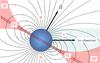 |
Fig. 1 A schematic sketch of a star with a global dipole magnetic field, illustrating the formation regions of different features in the spectrum of HD 54879. Region I: blue-shifted UV resonance line absorption (e.g., C iv, Si iv); Region II: UV resonance line emission; Region III: shocked, X-ray emitting region; Region IV: recombination line emission at the magnetic equator (Hα, Hβ). |
2. Observational data
We acquired three UV spectra of HD 54879 on April 30, 2016, using the HST high-resolution (R = 45 800) Space Telescope Imaging Spectrograph (STIS)1. The spectra cover the spectral range 1123–1710 Å. As no notable variability in the spectral lines could be identified, we co-added the three exposures to obtain a single spectrum with a signal-to-noise ratio S/N ≈ 100. While the exposures are flux calibrated, they have a significant offset relative to one another of the order of a factor of two, likely associated with light losses originating in thermal “breathing” that changes the focus over orbital time scales (Proffitt et al. 2017). The co-added spectrum was therefore recalibrated to match photometry from the TD-1 satellite (Thompson et al. 1978).
XMM-Newton observed HD 54879 on May 01, 2016 (PI: Hamann, ID: 0780180101) with an exposure time of ≈40 ks. All three European Photon Imaging Cameras (EPICs: MOS1, MOS2, and PN) were operated in the standard, full-frame mode with the medium UV filter. The observations were affected by periods of high flaring background, likely caused by soft protons populating Earth’s magnetosphere2. After excluding these periods, the useful exposure time was reduced to 29.8 ks. The data were reduced using the most recent calibration. The spectra and light curves were extracted using standard procedures from a region with a diameter of about 15′′. The background area was chosen to be nearby the star and free of X-ray sources.
Derived physical parameters for HD 54879.
Three spectropolarimetric observations of HD 54879 were obtained with the HARPS polarimeter (HARPSpol, Snik et al. 2008) attached to ESO’s 3.6 m telescope (La Silla, Chile) within ESO Large programme ID 191.D-0255 (PI Morel) on April 22, 2014 as well as on March 11 and 14, 2015. In this study, we make use only of the intensity spectra, which are of high resolution (R = 115 000), high (S/N ≈ 300), and cover the wavelength range 3780–6912 Å with a gap at 5259–5337 Å.
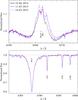 |
Fig. 2 The three HARPS observations focusing on Hα (upper panel) and a few photospheric lines (lower panel). |
To study the spectral variability, we employed 35 spectra from the Shenton Park Observatory (SPO) taken by Paul Luckas using a 0.35 m Ritchey-Chrétien telescope equipped with a Shelyak Lhires iii spectrograph operating at a resolution of R ≈ 16 000 and producing spectra with S/N ≈ 100. The spectra cover the spectral range 6500–6610 Å (Hα). Spectral images were bias-, dark-, and flat field corrected in the normal manner, and calibrated using Ne/Ar arc lamp spectra taken nightly and adjacent to science imaging. We also use seven spectra taken with the FEROS and FIES spectrographs from the IACOB and OWN projects (Barbá et al. 2010; Simón-Díaz et al. 2011a,b; Simón-Díaz & Herrero 2014) between the years 2009 and 2013 (see latter references for details). Together with the HARPS data, this makes a total of 45 spectra used to study the spectral variability. The spectra were cleaned from tellurics using the ESO tool Molecfit (Smette et al. 2015; Kausch et al. 2015) and rectified by eye. A log containing the epochs of observation is given in Table A.1.
For the spectral analysis, we also use UV photometry taken by the TD-1 satellite (Thompson et al. 1978), UBV photometry from Myers et al. (2003), R and JHKs 2MASS photometry from Zacharias et al. (2005), and I-band photometry from Monet et al. (2003).
3. Spectral analysis
With the goal of inferring the fundamental stellar and wind parameters, we now perform a consistent, multiwavelength analysis of the optical and UV spectra at hand. HD 54879 has previously been spectroscopically analyzed (C2015), but the analysis did not include UV data. The spectral modeling is performed with the PoWR model atmosphere code3. The PoWR code solves the radiative transfer and statistical equations in an expanding, spherically symmetric atmosphere, relaxing the assumption of local thermodynamic equilibrium (i.e., non-LTE). Indeed, the spherical symmetry in HD 54879 is broken by the presence of the strong magnetic dipole. A complete non-LTE solution of a magnetized stellar atmosphere in multiple dimensions is currently unfeasible. Nevertheless, our model provides a good approximation for the stellar photosphere, and can deliver significant insights on the stellar wind and mass-loss, as we show in the following sections. For more details on the PoWR code, we refer to Gräfener et al. (2002) and Hamann & Gräfener (2003).
By fitting synthetic spectra to the observations, we derive the effective temperature T∗, the surface gravity g∗, and the stellar luminosity L. The effective temperature T∗ refers to the stellar radius R∗, so that  . The stellar radius R∗ is defined at the model’s inner boundary, fixed at a mean Rosseland optical depth of τRoss = 20. The velocity field consists of two regimes. In the subsonic regime, hydrostatic equilibrium is approached (Sander et al. 2015). In the supersonic regime, the velocity follows the β-law with the value β = 0.8, typical for O-stars (Castor et al. 1975; Kudritzki et al. 1989; Puls et al. 1996). The co-moving frame radiative transfer is calculated adopting Gaussians for the absorption/emission coefficients with a constant Doppler width of vDop = 20 km s-1. During the calculation of the emergent spectrum, vDop is calculated via
  , where vth is the thermal velocity, and the microturbulent velocity ξ(r) is assumed to grow from the photospheric value ξph to the peak value ξmax at a prespecified radius Rξmax (see detailed in Shenar et al. 2015). A depth-dependent wind clumping is assumed here, reaching a maximum of D = 10. The synthetic profiles are convolved with Gaussians corresponding to the respective instrumental profiles. A comparison between the best-fitting model and the observations is shown in Fig. B.1. The derived stellar parameters are given in Table 1.
3.1. The stellar photosphere
Figure 2 shows several photospheric lines and the Hα line as observed in the three available HARPS spectra (see Table A.1). As the figure illustrates, the Hα line varies notably in shape, width, and equivalent width (EW). The intriguing three-peak profile of Hα is persistent in all observations. In contrast, no variability is detected in the photospheric features in the HARPS spectra. In fact, within the limitation set by the spectral resolution and S/N, no notable variability of the photospheric features is detected in the FEROS, FIES, or HARPS spectra taken between the years 2009 and 2015. He ii lines also show no evidence for variability, unlike in other massive magnetic stars (e.g., Grunhut et al. 2012; Hubrig et al. 2015b). Assuming that the star changes its orientation over the span of six years because of its rotation, this seems to suggest that the spherical symmetry of the photospheric layers is virtually unbroken by the presence of the magnetic field. Until evidence for photospheric variability is observed in HD 54879, a spherical symmetric model appears to be adequate for the analysis of its photosphere.
The surface gravity log g∗ is derived primarily from the pressure broadened wings of the Hγ and Hδ lines as well as He ii lines in the optical spectrum (see Fig. 3). Hα, and to a lesser extent Hβ, are strongly contaminated by emission originating at the magnetic equator (Sundqvist et al. 2012; ud-Doula et al. 2013). Since this is an inherently non-spherically symmetric structure (see Fig. 1 and Sect. 3.3), we do not attempt to include the disk emission in our model, and ignore Hα and Hβ for the estimation of log g∗. Our estimate for log g∗ is found to be consistent with the value reported by C2015.
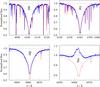 |
Fig. 3 Our best fitting model with parameters as in Table 1 (red dotted line) compared to the first four Balmer lines, as observed in the HARPS spectrum (blue solid line). The disk emission of Hα and Hβ is not included in the model. |
The temperature is determined from the ratios between lines from different ionization stages of the same element, for example, He i/ii (see Fig. 4), N ii/iii/iv, and C ii/iii/iv. The temperature we obtain (30.5 ± 0.5 kK) is significantly lower than that derived by C2015 (33 ± 1 kK). We note, however, that the temperature derived here is more consistent with our target’s spectral type, O 9.7 V, considering calibrations by Martins et al. (2005a). Moreover, a comparison of the observed photospheric spectra with TLUSTY model atmospheres (Hubeny & Lanz 1995; Lanz & Hubeny 2003) implies a similar temperature to that derived here.
By fitting the star’s spectral energy distribution (SED), we derive the luminosity L and reddening EB−V (see upper panel of Fig. B.1). Different extinction laws were tested, and the SED is best reproduced using laws published by Seaton (1979) and Nandy et al. (1975). The luminosity derived here agrees well with C2015 when scaling L ∝ d2 to the distance used by C2015 (d = 1.32 kpc), which is likely overestimated (see discussion on the distance in Sect. 1).
Finally, having constrained the fundamental parameters of the star, the abundances are inferred from the overall strength of spectral lines belonging to the corresponding element. Abundances that could not be derived due to the absence of corresponding spectral lines are assumed to have solar values (Asplund et al. 2009). The derived/adopted values are given in Table 2. We can exclude a significant overabundance of He compared to the solar value. Our results agree well with those by C2015, within errors. It is interesting to note that both C and N are found to be significantly subsolar, standing in contrast to reports of nitrogen enhancement in magnetic B-type stars (e.g., Morel et al. 2008).
Derived chemical abundances (in mass fractions) for HD 54879.
3.2. Rotation and turbulence
Any periodicities observed in our target are likely to correlate with its rotational period Prot. It is therefore important to constrain the projected rotational velocity vsini from our high-resolution spectra. C2015 used the Fourier tool iacob-broad (Simón-Díaz & Herrero 2014) to derive a projected rotational velocity of vsini = 7 ± 2 km s-1. However, for rotational velocities that are comparable to the microturbulent velocity, the tool strongly underestimates the involved errors, making it inapplicable for HD 54879 (see discussion by Simón-Díaz & Herrero 2014, Sect. 3.4). Constraining vsini is difficult, because its associated spectral line broadening “competes” with the microturbulent velocity ξph, the macroturbulent velocity vmac, and the thermal velocity vth = 2kBT/m. To overcome this, we consider first spectral lines belonging to CNO ions. For these elements, vth ≈ 6−7 km s-1, which alone agrees with the observed line widths. Therefore, the unknowns ξph, vsini, and vmac must be smaller than vth.
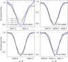 |
Fig. 5 Selected CNO spectral lines of our best fitting model convolved with rotation profiles for vsini = 0,4, and 8 km s-1 (red, green, and black dotted lines, respectively), compared to observations (blue solid line). |
Figure 5 displays selected CNO spectral lines compared to our best fitting model convolved with rotation profiles of different vsini values (see legend and caption) calculated with ξph = 0 km s-1. It is evident that, for the majority of spectral lines, no broadening mechanism beyond those which are included in the calculation are required. Figure 5 shows that we can only hope to derive an upper limit for the projected rotation velocity. Based on our study, we can constrain this limit to vsini ≤ 4 km s-1.
The microturbulence could only be estimated approximately from the UV iron lines, which are subject to low thermal broadening (vth ≈ 3 km s-1) . We estimate ξph ≈ 3 km s-1, but can only reliably constrain an upper limit of ξph ≤ 4 km s-1. Similarly, we can conclude vmac ≤ 4 km s-1, as opposed to vmac = 8 km s-1 reported by C2015.
The small value of vmac derived here stands in contrast to the significant macroturbulent velocities reported for other magnetic O-type stars (Sundqvist et al. 2013). A very low macroturbulent velocity (<3 km s-1) was reported by the latter authors only for the strongly magnetized star NGC 1624-2. However, Sundqvist et al. (2013) showed that this can be understood as a consequence of its extraordinary magnetic field (Bd = 20 kG), which is strong enough to stabilize the atmosphere at deep sub-photospheric layers, where the iron opacity peak is reached and macroturbulence is thought to originate (e.g., Cantiello et al. 2009). The same argument does not hold for our target given its much weaker magnetic field. Rather, we suggest that the small value found here for HD 54879 is related to its low effective temperature (compared to the sample analyzed by Sundqvist et al. 2013). τ Sco is another magnetic star of a similar spectral type and magnetic field strength for which a low macroturbulent velocity was reported (Smith & Karp 1978). Recent studies by Simón-Díaz et al. (2017) imply that late-type massive stars exhibit systematically lower macroturbulent velocities compared to early-type stars, although the large scatter in vmac values prevents us from concluding this unambiguously.
3.3. The stellar wind
Empirically derived mass-loss rates of low luminosity (log Lbol/L⊙< 5.2) OB-dwarfs are orders of magnitude lower than predicted by standard mass-loss recipes (Bouret et al. 2003; Martins et al. 2005b; Marcolino et al. 2009; Oskinova et al. 2011; Huenemoerder et al. 2012). This is often referred to in the literature as the weak wind problem.
There are various explanations as to why measured mass-loss rates of OB-dwarfs are so low. Some authors suggest that the wind-driving force in OB dwarfs is lower than predicted by current models, and that their winds are genuinely weak. For example, Drew et al. (1994) proposed that the ionization of winds by X-rays reduces the total radiative acceleration. However, Oskinova et al. (2011) showed that ionization by X-rays does not significantly inhibit the wind driving power in magnetic B-dwarfs. An alternative idea was proposed by Lucy (2012), who suggested that, in late-type O dwarfs, the shock-heating of the ambient gas results in a single-component flow with a temperature of a few MK. This hot wind coasts to high velocities as a pure coronal wind. Hence, the bulk of the wind is not visible in the optical/UV, and mass-loss rates derived from these spectral ranges are not reliable. High-resolution X-ray spectroscopy of O-dwarfs seem to support this scenario (e.g., Huenemoerder et al. 2012, and references therein).
A comparison of HST UV data of the prototypical O9.7 V star υ Ori (HD 36512) with the HST data collected for our target, HD 54879, is shown in Fig. 6, where we focus on the two most prominent wind features, the resonance lines C iv λλ1548,1551 and Si iv λλ1394,1403. It is evident that υ Ori shows no, or very little, evidence for a stellar wind. Assuming υ Ori has the same fundamental parameters as HD 54879, and adopting a terminal velocity of v∞ = 1700 km s-1 (Kudritzki & Puls 2000), a quick analysis of its UV spectrum using the PoWR code suggests an upper limit of log Ṁ ≲ −9.3 [M⊙ yr-1] for υ Ori. This is lower by almost two orders of magnitude compared to predictions by Vink et al. (2000), following the trend of other weak-wind stars.
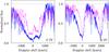 |
Fig. 6 Comparison of normalized HST observations of the prototypical O9.7 V star HD 36512 (ID: 13346, PI: Ayres, pink solid line) and of HD 54879 (blue solid line) in Doppler space. Shown are the resonance lines C iv λλ1548,1551 (left panel) and Si iv λλ1394,1403 (right panel). |
In contrast to υ Ori, our target shows a clear asymmetry that is suggestive of absorption stemming from matter surrounding the star. At first glance, this seems to suggest that the magnetic field in fact spurs mass-loss from the star, contrary to expectation. However, the profiles of the resonance lines of HD 54879 have unusually shallow blueshifted edges, suggesting the presence of a large velocity dispersion, reaching a maximum speed of ≈1000 km s-1. Similar line profiles were reported in other studies of magnetic stars (e.g., Marcolino et al. 2013; Nazé et al. 2015).
The magnetic field in HD 54879 dominates the behavior of the stellar wind for radii smaller than the Alfvén radius rA, which is estimated to rA ≳ 12 R∗ in this work (see below). To understand the line profiles of the Si iv and C iv resonance lines (Fig. 6), as well as the prominent Hα emission (Fig. 3), we refer the reader to Fig. 1. The absorption of the UV resonance lines is mostly blueshifted, because it is formed in front of the stellar disk, where the material moves mostly towards the observer (region I). Some emission in the resonance lines (blueshifted and redshifted) is formed in the less dense region II, but it competes with line absorption originating in the stellar photosphere. Moreover, X-rays formed in region III (Owocki et al. 2016) ionize the Si iv and C iv ions and reduce their emissivity/opacity. Finally, as a recombination line, the emission in Hα scales with ρ2, ρ being the density. Therefore, Hα emission stems primarily from the magnetic equator (region IV), where ρ is orders of magnitudes larger. In case of a pronounced shock retreat, the formation of a disk-like structure may be inhibited (ud-Doula et al. 2014). However, Hα is still expected to trace dense environments that strongly deviate from spherical symmetry, and is therefore not modeled in the framework of this study. Both the dynamic nature of the disk as well as possible co-rotation contribute to the width of the Hα feature. The presence of Hα emission or broadened, asymmetric lines in the UV is therefore not related to the stellar wind, but to the magnetosphere, and they do not imply a mass-loss from HD 54879 (see also Nazé et al. 2015; Erba et al. 2017).
To illustrate the inability of a standard, spherically-symmetric outflow to reproduce the observations, we plot in Fig. 7 several synthetic spectra calculated with the parameters given in Table 1, but with v∞ = 900 km s-1 (roughly corresponding to the observed blue edge of the lines), a standard wind turbulent velocity (0.1 v∞), and different mass-loss rates. It is evident from the figure that no combination of wind parameters can reproduce the observed shallow profiles, which indicates that the stellar wind is heavily affected by the magnetic field.
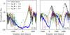 |
Fig. 7 Normalized HST observations of HD 54879 (blue solid line) compared to synthetic spectra with a terminal velocity of v∞ = 900 km s-1 and different mass-loss rates (given in the legend in [M⊙ yr-1]). |
Solving the full non-LTE radiative transfer in the presence of a magnetic field in 3D is currently not feasible and beyond the scope of this study. Instead, we simulate the motion of the matter along the field lines by a turbulent velocity which is strongly enhanced close above the stellar surface, at r ≈ 1.1 R∗. We find the best fit for the combination of v∞,sph = 300 km s-1, ξwind,sph = 500 km s-1, and log Ṁsph = −8.8 [M⊙ yr-1]. X-rays ionization is approximately accounted for in a spherically-symmetric fashion (see Sect. 3.4). The results are shown in Fig. 8. We note that these parameters do not correspond to actual physical parameters, since they are obtained via a spherically symmetric model which assumes a constant outflow. Rather, these parameters serve to reproduce the conditions in the formation region of the resonance lines. For example, the model predicts that the density at the main line forming region, at r ≈ 1.1−2 R∗, is ρ ≈ 10-15−10-16 g cm-3.
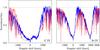 |
Fig. 8 Normalized HST observations of HD 54879 (blue solid line) compared to our best-fitting model, which accounts for a large microturbulence and superionization by X-rays. |
By comparing the derived densities to predictions by an analytical model derived for stars with a constant outflow and a global dipole magnetic field (Owocki et al. 2016), we can provide a rough estimate of the mass-loss rate that HD 54879 would have in the absence of a magnetic field, ṀB = 0. This model assumes three components: (a) an upflow along the dipole lines towards the loop apex; (b) a shocked, X-ray-emitting plasma; and (c) a cooled downflow from the dipole apices back towards the star. Assuming simplistically a β-type law for the expansion speed, the model predicts the densities ρu, ρs, and ρd (Eqs. (10), (20), and (25) in Owocki et al. 2016) as a function of the polar coordinates (r,θ) of the upflowing, shocked, and downflowing plasma as a function of v∞, R∗, M∗, and ṀB = 04. Since the P-Cygni absorption originates in the upflowing and downflowing plasma in the magnetosphere, we compare the densities derived from our spherical models with the sum ρu + ρd. Evaluating this for a typical viewing angle of θ = 60° at different radii between 1.1 and 2.0 R∗, and assuming v∞ = 1700 km s-1 and the parameters derived in our model, we obtain values for log ṀB = 0 that range between −9.2 and −8.8 [M⊙ yr-1]. This is smaller than the values predicted by Vink et al. (2000) (≈−7.7 [M⊙ yr-1]) by more than an order of magnitude, but in line with values reported for other stars of similar spectral type (e.g., Marcolino et al. 2009).
Since our radiative transfer assumes spherical symmetry, our result should be considered as an order-of-magnitude estimate (±0.5 dex), and not as an accurate derivation of log ṀB = 0. From log ṀB = 0 ≈ −9.0 [M⊙ yr-1] and Bd ≳ 2 kG, and assuming again v∞ = 1700 km s-1, we can constrain the Alfvén radius to rA ≳ 12 R∗. From this, we can then estimate the true mass-loss from the star to log Ṁ ≲ −10.2 [M⊙ yr-1] (see Eqs. (1)–(3) of Petit et al. 2017). However, we cannot exclude the possibility that some mass is lost from the star as a hot, X-ray emitting wind.
Importantly, while the magnetic field suppresses mass-loss from the star, it causes a density enhancement around it that leaves a spectroscopic signature. Therefore, the analysis of massive magnetic stars using appropriate models may enable one, in principle, to predict the mass-loss rates of non-magnetic stars of a similar spectral type, which cannot be measured otherwise. Magnetic stars can therefore help to resolve the weak-wind problem.
3.4. The effect of X-rays on the stellar wind
The X-rays present in the stellar atmosphere are expected to affect the ionization balance via K-shell Auger ionization (Auger 1923). This effect is known to lead to high ionization stages such as N v and O vi (Cassinelli & Olson 1979; Oskinova et al. 2011). Moreover, X-rays affect diagnostic wind lines such as the resonance lines of C iv and Si iv. In our case, the N v λλ1239,1243 resonance lines are clearly present in the HST data, while our model predicts that N v is not significant in the stellar wind when not including X-rays. This suggests that X-rays contribute to the appearance of the UV spectrum.
Auger ionization via X-rays is accounted for in our model by assuming optically thin, thermally emitting filaments of shocked plasma embedded in the wind (Baum et al. 1992). While the topology of the X-ray emitting plasma may be more complex in reality, the important quantity here is merely the amount of ionizing radiation. The observed X-ray spectrum is characterized by two temperature components TX,1 and TX,2 and corresponding filling factors Xfill,1 and Xfill,2. These parameters are adopted from our analysis presented in Sect. 5, where only the two dominant components are accounted for. The onset radius of these filaments is set to R0 = 1.05 R∗. Slightly different values deliver similar results, but onset radii which are too large trivially do not affect the spectra.
In Fig. 9, we compare the HST observations of the N v λλ1239,1243 and Si iv λλ1394,1403 resonance lines to our best-fitting model with and without X-rays. As discussed above, the N v resonance doublet is clearly seen in the observations but not in the model without X-rays. With the inclusion of X-rays, the N v lines appear. The N v line profiles have a similar shape to the C iv and Si iv resonance lines, suggesting that they too form in the magnetosphere. The strength of the lines implies a nitrogen abundance slightly lower than derived from our photospheric analysis by a factor of ≈0.7, but this is within our given uncertainty. The X-rays also significantly influence the resonance lines of Si iv (see Fig. 9, right panel) and C iv. Including X-rays, our model successfully reproduces the main characteristics of our observations.
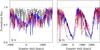 |
Fig. 9 Normalized HST observations of HD 54879 (blue solid line) compared to our best-fitting model (red dotted line) and to the same model without the inclusion of X-rays (black dashed line). |
4. Evolutionary status
Using the parameters given in Table 1, we can derive an evolutionary scenario for HD 54879. Here, we use the BONNSAI5 tool (Schneider et al. 2014), which implements Bayesian statistics on a set of evolutionary tracks for massive stars (Brott et al. 2011) to constrain the best-fitting evolutionary channel. Previously performed by C2015, we repeat this procedure in light of the different parameters derived in this study. The parameters used are log L,log T, and log g∗. The errors for log T∗ and log g∗, and log L are taken from Table 1. The peculiar C and N abundances are ignored.
Our BONNSAI solution predicts an initial mass of Mini = 16 ± 1 M⊙ and an age of 5 ± 1 Myr. Our results are consistent with the findings by C2015 within errors. We do not find any indication that a merger event was involved in the formation of HD 54879, such as rejuvenation or rapid rotation. Nevertheless, traces for a past merger event may be unobservable if it occurred several million years ago.
We note that the evolution models used by the BONNSAI tool do not include the effect of magnetic fields. Thus, in addition to the uncertainties involved in evolution models of massive stars (e.g., overshooting, mass-loss rates), systematic errors due to the omission of magnetic fields in the models may interfere with our results. For example, according to our results in Sect. 3.3, HD 54879 loses significantly less mass than assumed by the BONNSAI evolution tracks. Because the magnetic field is known to strongly dampen the surface rotation, and in light of the very low vsini value measured in this work, we used tracks which neglect rotationally induced mixing by setting the equatorial rotational velocity to zero (vrot,ini = 0 km s-1).
5. X-ray spectral analysis
To analyze the XMM-Newton spectra, we used the standard spectral fitting software xspec (Arnaud 1996). The abundances were adopted from our spectral analysis in Sect. 3 (cf. Table 2). The X-ray flux of HD 54879 in the 0.2–12 keV band measured by the XMM-Newton is ≈2 × 10-13 erg cm-2 s-1 (see Table 3). The unabsorbed flux corresponds to an X-ray luminosity at a distance of 1.0 kpc log LX ≈ 32.0 erg s-1, resulting in log LX/Lbol ≈ −6 (cf. Table 1). This is a higher value compared to other stars with similar spectral types. For example, the X-ray luminosity and the temperature of the hottest plasma found in μ Col (O9.5 V), ζ Oph (O9.2I V), 10 Lac (O9 V), σ Ori (O9.5 V), and other non-magnetic late O-dwarfs are at least an order of magnitude lower than in HD 54879 (Oskinova et al. 2006; Waldron & Cassinelli 2007; Huenemoerder et al. 2012).
In contrast, all known magnetic O-dwarfs – θ1 Orionis C (O7 Vp), Tr 16-22 (O8.5 V), HD 57682 (O9.5 V), τSco – have relatively hard X-ray spectra and X-ray luminosities ≳1032 erg s-1, similar to HD 54879 (Schulz et al. 2000; Nazé et al. 2014). Thus, it appears safe to conclude that there is a clear dichotomy in the X-ray properties among non-magnetic and magnetic O-dwarfs, with the latter being significantly more X-ray luminous and displaying harder X-ray spectra than the former (the situation may be more complex in case of OB-supergiants and Of?p stars, see recent reviews by Nazé et al. 2014; ud-Doula & Nazé 2016). On this basis, we attribute the relatively high X-ray luminosity of HD 54879 to its magnetic nature.
It order to establish the temperature of the X-ray-emitting plasma, we have analyzed the observed low-resolution XMM-Newton spectra of HD 54879 (high-resolution RGS spectra have an insufficient signal and are not useful). The X-ray spectra of magnetic hot stars are usually well described by multi-temperature thermal plasma models (e.g., Oskinova et al. 2011; Nazé et al. 2014). This is also the case for HD 54879.
As a first step, we fitted the observed spectra in the 0.2–10.0 keV band with a thermal two-temperature spectral model that assumes optically thin plasma in collisional equilibrium. At this step, the absorption was modeled as originating in the cold interstellar medium (Wilms et al. 2000). The resulting spectral fit is statistically significant, with a reduced χ2 = 1.3. The best fit parameters are shown in Table 3.
There is no physical motivation for restricting the plasma temperature distribution to two temperatures. In fact, spectroscopic analyses show a continuous temperature distribution in hot stars (Wojdowski & Schulz 2005). Therefore, as a next step, we fitted a three-temperature spectral model to the observed EPIC spectra of HD 54879. Also in this case, the fit is statistically significant, with χ2 = 1.1. The three-temperature model fit is shown in Fig. 10, and the associated parameters are shown in Table 3. The three-temperature fit reveals the hottest plasma component with a temperature of about 2 keV (~20 MK). Better S/N is required to confirm the presence of this high-temperature plasma. We also tried to fit a four-temperature plasma model. However, the quality of the data is not sufficient to further constrain the temperature distribution.
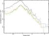 |
Fig. 10 XMM-Newton PN, MOS1, and MOS2 spectra of HD 54879 (black, red, and green curves, respectively) with error bars corresponding to 3σ with the best fit three-temperature thermal model (solid lines). The model parameters are shown in Table 1. |
X-ray spectral parameters derived from the XMM-Newton observations of HD 54879 assuming a three-temperature plasma model.
In the framework of the magnetically confined wind shocks (MCWS) model (Babel & Montmerle 1997; ud-Doula & Owocki 2002), the wind plasma streams collide at the magnetic equator and give rise to a shock that heats the plasma. Hence, the maximum temperature follows from a Rankine-Hugoniot condition and cannot exceed a value determined by the maximum streaming velocity. Motivated by the recent discovery of a non-thermal component in the X-ray emission of the magnetic star HR 7355 (Leto et al. 2017), we also fitted the observed spectra with a composite two-temperature thermal plasma and a non-thermal, power law component. The model provides a fit of similar quality to the observed spectra (χ2 = 1.2 for 138 degrees of freedom). The best fit thermal plasma temperatures are kT1 = 0.18 ± 1.2 [keV], kT2 = 0.74 ± 0.02 [keV], and the power-law exponent is Γ = 2.5 ± 0.7. Thus, the quality of the data is not sufficient to discriminate between three-temperature thermal and two-temperature thermal plus non-thermal component models.
Interestingly, the total absorption derived from our X-ray analysis is found to be somewhat higher than that derived from the analysis of UV and optical data (Sect. 3). Using the averaged relation NH = EB−V·6 × 1021 cm-2 (Gudennavar et al. 2012), EB−V = 0.35 implies NH,ISM = 2.1 × 1021 cm-2, which is lower by almost a factor of two compared to what is found from the X-ray data (see Table 3). Since the absorption derived from X-rays includes both interstellar and intrinsic absorption, it is possible that the additional X-ray absorption occurs in the magnetosphere of HD 54879. Alternatively, this discrepancy could be merely a consequence of the large error on NH (see Table 3) when derived from our low-resolution X-ray spectra, and of the uncertain relations between NH, EB−V, and the extinction parameters AV and RV (e.g., Güver & Özel 2009).
To test whether or not some X-ray absorption originates in the magnetosphere, we searched for the presence of absorption edges corresponding to the leading ionization stages of abundant metals in HD 54879. Fitting the observed spectra with an absorption model that includes multiple ions did not statistically improve the fit. Hence, we concentrated on searching absorption edges of individual ions. Fitting a three-temperature plasma model that, in addition to the interstellar absorption, is also attenuated by a “warm” absorber resulted in a detection of an absorption edge at 0.61 ± 0.15 keV with an optical depth 0.9 ± 0.6. This energy corresponds to the absorption edges of O iii-vii (Verner & Yakovlev 1995). The fact that these are leading ionization stages of oxygen in the magnetosphere of HD 54879 provides additional support for the detection of the absorption edge. Including ionization edges in the X-ray spectral model does not significantly affect the derived value of the total ISM absorption NH,ISM. Hence, while the data agree with some X-ray absorption due to the warm material trapped in the magnetosphere, the quality of our data prevents us from measuring the warm absorption component unambiguously.
In Sect. 3.3, we showed that the true wind parameters (Ṁ,v∞) cannot be derived for this object based on UV/optical spectra. However, as suggested by Lucy (2012), it is possible that a significant amount of matter leaves the star in a very hot phase and emits in X-rays. From high-resolution X-ray spectra, one could study in detail the properties of the stellar wind of the HD 54879, if it indeed exists. To shed light on the urgent weak wind problem, as well as on the true mass-loss rates of massive main sequence stars, we therefore encourage future observational campaigns to acquire high-resolution X-ray spectra for HD 54879.
6. Variability
6.1. Photometric variability
In Fig. 11, we present a light curve collected by the All Sky Automated Survey 3 (ASAS3, six-pixel wide aperture) for our target (Pojmanski 2002). The dataset was scanned for significant periods using Fourier and F-statistics, but none could be identified. Striking are the sudden decreases in brightness, which only last for ≈1 d, evident in Fig. 11. We checked whether these events occur periodically and can safely reject this possibility, excluding binary eclipses as a possible explanation. Sudden brightness changes could also arise from outbursts. However, the intensity of change in magnitude and the short time scale over which these events occur do not plausibly agree with such a model. Similar outliers can be seen in other light curves obtained by the ASAS (e.g., Paczyński et al. 2006). We conclude that these events are most likely observational artefacts.
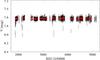 |
Fig. 11 ASAS3 light curve of HD 54879. |
6.2. Spectroscopic variability
HD 54879 appears to exhibit both small-scale and large-scale variability that are especially evident in the Hα line (see Fig. 2). While the dynamic structure of the magnetosphere implies some stochastic variability (e.g., Sundqvist et al. 2012; ud-Doula et al. 2013), it is also expected that a periodic variability that correlates with the rotational period of the star should be present (e.g., Stibbs 1950; Townsend & Owocki 2005; Wade et al. 2011).
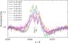 |
Fig. 12 FEROS, FIES, and HARPS spectra of Hα taken in the years 2009–2015 (see legend and Table A.1). |
To illustrate the short-scale variability, we refer the reader to Fig. 2 in Sect. 3. The figure shows that, while Hα maintains a similar equivalent width between 11-03-2015 and 14-03-2015, some variability can be seen in the strength of the leftmost emission peak and the right absorption wing. In other words, the star exhibits some variability on the scale of days, which can be considered short-scale in our context. The third spectrum, taken about half a year prior to the others (April 22, 2014), shows a higher equivalent width (less emission) and a narrower profile. This suggests that a mechanism is present that is responsible for long-term variability. Figure 12 shows nine spectra of Hα taken in the years 2009–2015 (see Table A.1 and legends). One can see clear changes in the equivalent widths and full widths at half maximum (FWHM) of the profiles, as well as differing strengths of the absorption wings.
These spectra alone are not sufficient to determine a period. For this reason, we acquired 35 amateur spectra (P. Luckas, priv. comm.) collected specifically for this project (see Sect. 2). The spectra are of lower quality, but offer the advantage of a much denser time coverage. A few selected spectra are shown in Fig. 13.
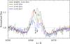 |
Fig. 13 A few amateur SPO spectra of Hα, shown with a single HARPS spectrum for comparison. |
It is not trivial to identify the quantity whose time series would best constrain a period for the global variability. A rotational modulation can lead to a partial polar/equatorial view (relative to the magnetic axis) of the disk-like, Hα emitting structure, which in turn leads to a periodic variation in the equivalent widths (e.g., Sundqvist et al. 2012; ud-Doula et al. 2013). We therefore measured the equivalent width of the Hα line in the range 6551–6576 Å in all available spectra. The error bars are attributed mostly to uncertainty in rectification, and are roughly estimated by Δλ/S/N, where Δλ = 25 Å is the integration domain. The results are listed in Table A.1 and shown in Fig. 14.
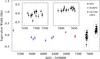 |
Fig. 14 Equivalent widths of Hα versus heliocentric Julian date, as measured in the IACOB/OWN, HARPS and amateur SPO spectra. |
Figure 14 seems to be suggestive of a modulation of the equivalent widths over a very long period, of the order of years. A Fourier analysis of the signal (Scargle 1982; Horne & Baliunas 1986) suggests a period of ≈5 yr as the only significant period. This result is consistent with the upper limit of vsini< 4 km s-1 derived in Sect. 3. From the derived period and stellar radius, and assuming the probable value i ≈ 60°, this suggests a very low rotational velocity of veq ≈ 0.2 km s-1. Additional attempts to constrain the period using other proxies such as the line width or its centroid did not result in any coherent periods. We therefore suggest in this paper a rotational period of ≈5 yr, but more spectra will be necessary to validate our claim. Overall, this result is consistent with the fact that magnetic stars are very slow rotators that have lost their angular momentum via magnetic braking (Weber & Davis 1967; ud-Doula & Owocki 2002).
7. Summary
We performed a comprehensive, multiwavelength analysis of HD 54879 (O9.7 V). With a dipole magnetic field of Bd ≳ 2 kG, it is one of about ten magnetized O-stars known. Using high-quality X-ray, UV, and optical spectra acquired by the XMM-Newton, HST, and HARPS instruments, respectively, we could derive the X-ray properties of HD 54879 and analyze its atmosphere and wind. Moreover, 45 spectra were used to constrain a periodic variability of the Hα line. We conclude the following:
-
The fundamental stellar parameters (T∗,L,log g) ofHD 54879 are typical for its spectral type.Nitrogen and carbon abundances are found to be subsolar.
-
The projected rotational velocity vsini, the microturbulent velocity ξph, and the macroturbulent velocity vmac, are all found to be smaller than 4 km s-1.
-
The X-ray spectrum can be well-fitted with a thermal model accounting for either two or three components, and implies a higher-than-average X-ray luminosity (log LX/Lbol = −6.0). In the three-component model, the X-ray temperature reaches values up to TX ≈ 20 MK.
-
Variability of Hα equivalent widths is suggestive of a very long period of the order of ≈5 yr, consistent with the low vsini value.
-
The mass-loss rate that our target would have in the absence of a magnetic field could be roughly estimated to be log ṀB = 0 ≈ −9.0 [M⊙ yr-1]. This is significantly less than theoretically predicted (Vink et al. 2000), but is in line with what is found for non-magnetic stars of similar spectral types (Marcolino et al. 2009). With an Alfvén radius of rA ≳ 12 R∗, the true mass-loss rate of HD 54879 is estimated as log Ṁ ≲ −10.2 [M⊙ yr-1].
To conclude, we would like to point out that, as our study illustrates, slowly rotating magnetic stars can provide important constraints on the weak wind problem. The spectra of main sequence OB-type stars often exhibit very little or no signatures for a stellar wind in UV spectra, which contain the principle diagnostics for mass-loss rates. Magnetic fields that confine the stellar winds enhance the circumstellar densities and result in clear spectral features. Using sophisticated models for the magnetospheres of massive magnetic stars, one can therefore infer values for log ṀB = 0. These should be similar to true mass-loss rates for non-magnetic main sequence stars of the same spectral type.
Based on observations made with the NASA/ESA Hubble Space Telescope, obtained at the Space Telescope Science Institute, which is operated by the Association of Universities for Research in Astronomy, Inc., under NASA contract NAS 5-26555. These observations are associated with the proposal ID 14480, PI: Hamann.
See XMM-Newton Users Handbook.
PoWR models of Wolf-Rayet and OB-type stars can be downloaded at www.astro.physik.uni-potsdam.de/PoWR
The model also introduces the parameter δ which describes the location of onset of matter infall along the dipole loop. The impact of this parameter is, for our estimation, negligible.
The BONNSAI web-service is available at www.astro.uni-bonn.de/stars/bonnsai
Acknowledgments
T.S. and L.O. acknowledge support from the german “Verbund- forschung” (DLR) grants 50 OR 1612 and 50 OR 1302. A.S. is supported by the Deutsche Forschungsgemeinschaft (DFG) under grant HA 1455/26. The IACOB spectroscopic database is based on observations made with the Nordic Optical Telescope (www.not.iac.es) operated by the Nordic Optical Telescope Scientific Association, and the Mercator Telescope (www.mercator.iac.es), operated by the Flemish Community, both at the Observatorio de El Roque de los Muchachos (www.iac.es) (La Palma, Spain) of the Instituto de Astrofísica de Canarias (www.iac.es). This research has made use of the VizieR catalogue access tool, CDS, Strasbourg, France. The original description of the VizieR service was published in Ochsenbein et al. (2000). We thank our referee, G. Wade, for his constructive and careful reviewing of our manuscript.
References
- Alecian, E., Kochukhov, O., Petit, V., et al. 2014, A&A, 567, A28 [NASA ADS] [CrossRef] [EDP Sciences] [Google Scholar]
- Arnaud, K. A. 1996, in Astronomical Data Analysis Software and Systems V, eds. G. H. Jacoby, & J. Barnes, ASP Conf. Ser., 101, 17 [Google Scholar]
- Asplund, M., Grevesse, N., Sauval, A. J., & Scott, P. 2009, ARA&A, 47, 481 [NASA ADS] [CrossRef] [Google Scholar]
- Auger, P. 1923, C.R.A.S. Paris, 177, 169 [Google Scholar]
- Babel, J., & Montmerle, T. 1997, A&A, 323, 121 [NASA ADS] [Google Scholar]
- Barbá, R. H., Gamen, R., Arias, J. I., et al. 2010, Rev. Mex. Astron. Astrofis. Conf. Ser., 38, 30 [NASA ADS] [Google Scholar]
- Baum, E., Hamann, W.-R., Koesterke, L., & Wessolowski, U. 1992, A&A, 266, 402 [NASA ADS] [Google Scholar]
- Bouret, J.-C., Lanz, T., Hillier, D. J., et al. 2003, ApJ, 595, 1182 [NASA ADS] [CrossRef] [Google Scholar]
- Brott, I., Evans, C. J., Hunter, I., et al. 2011, A&A, 530, A116 [NASA ADS] [CrossRef] [EDP Sciences] [Google Scholar]
- Cantiello, M., Langer, N., Brott, I., et al. 2009, A&A, 499, 279 [NASA ADS] [CrossRef] [EDP Sciences] [Google Scholar]
- Cassinelli, J. P., & Olson, G. L. 1979, ApJ, 229, 304 [NASA ADS] [CrossRef] [Google Scholar]
- Castor, J. I., Abbott, D. C., & Klein, R. I. 1975, ApJ, 195, 157 [NASA ADS] [CrossRef] [Google Scholar]
- Castro, N., Fossati, L., Hubrig, S., et al. 2015, A&A, 581, A81 [NASA ADS] [EDP Sciences] [Google Scholar]
- Clariá, J. J. 1974, A&A, 37, 229 [NASA ADS] [Google Scholar]
- Crowther, P. A., & Hadfield, L. J. 2006, A&A, 449, 711 [NASA ADS] [CrossRef] [EDP Sciences] [Google Scholar]
- Donati, J.-F., & Landstreet, J. D. 2009, ARA&A, 47, 333 [NASA ADS] [CrossRef] [MathSciNet] [Google Scholar]
- Donati, J.-F., Babel, J., Harries, T. J., et al. 2002, MNRAS, 333, 55 [NASA ADS] [CrossRef] [MathSciNet] [Google Scholar]
- Drew, J. E., Hoare, M. G., & Denby, M. 1994, MNRAS, 266, 917 [NASA ADS] [CrossRef] [Google Scholar]
- Eldridge, J. J., & Stanway, E. R. 2016, MNRAS, 462, 3302 [NASA ADS] [CrossRef] [Google Scholar]
- Erba, C., David-Uraz, A., Petit, V., & Owocki, S. P. 2017, ArXiv e-prints [arXiv:1702.08535] [Google Scholar]
- Ferrario, L., Pringle, J. E., Tout, C. A., & Wickramasinghe, D. T. 2009, MNRAS, 400, L71 [NASA ADS] [CrossRef] [Google Scholar]
- Fossati, L., Castro, N., Schöller, M., et al. 2015, A&A, 582, A45 [NASA ADS] [CrossRef] [EDP Sciences] [Google Scholar]
- Friend, D. B., & MacGregor, K. B. 1984, ApJ, 282, 591 [NASA ADS] [CrossRef] [Google Scholar]
- Gaia Collaboration (Brown, A. G. A., et al.) 2016, A&A, 595, A2 [NASA ADS] [CrossRef] [EDP Sciences] [Google Scholar]
- Georgy, C., Ekström, S., Meynet, G., et al. 2012, A&A, 542, A29 [NASA ADS] [CrossRef] [EDP Sciences] [Google Scholar]
- Gräfener, G., Koesterke, L., & Hamann, W.-R. 2002, A&A, 387, 244 [NASA ADS] [CrossRef] [EDP Sciences] [Google Scholar]
- Gregorio-Hetem, J. 2008, in Handbook of Star Forming Region, Vol. II, ed. B. Reipurth (ASP Monograph Publications), 1 [Google Scholar]
- Grunhut, J. H., Wade, G. A., Marcolino, W. L. F., et al. 2009, MNRAS, 400, L94 [NASA ADS] [CrossRef] [Google Scholar]
- Grunhut, J. H., Wade, G. A., Sundqvist, J. O., et al. 2012, MNRAS, 426, 2208 [NASA ADS] [CrossRef] [Google Scholar]
- Grunhut, J. H., Wade, G. A., Neiner, C., et al. 2017, MNRAS, 465, 2432 [NASA ADS] [CrossRef] [Google Scholar]
- Gudennavar, S. B., Bubbly, S. G., Preethi, K., & Murthy, J. 2012, ApJS, 199, 8 [NASA ADS] [CrossRef] [Google Scholar]
- Güver, T., & Özel, F. 2009, MNRAS, 400, 2050 [NASA ADS] [CrossRef] [Google Scholar]
- Hainich, R., Pasemann, D., Todt, H., et al. 2015, A&A, 581, A21 [Google Scholar]
- Hamann, W.-R., & Gräfener, G. 2003, A&A, 410, 993 [NASA ADS] [CrossRef] [EDP Sciences] [Google Scholar]
- Horne, J. H., & Baliunas, S. L. 1986, ApJ, 302, 757 [NASA ADS] [CrossRef] [Google Scholar]
- Hubeny, I., & Lanz, T. 1995, ApJ, 439, 875 [Google Scholar]
- Hubrig, S., Schöller, M., Kharchenko, N. V., et al. 2011, A&A, 528, A151 [NASA ADS] [CrossRef] [EDP Sciences] [Google Scholar]
- Hubrig, S., Schöller, M., Fossati, L., et al. 2015a, A&A, 578, L3 [NASA ADS] [CrossRef] [EDP Sciences] [Google Scholar]
- Hubrig, S., Schöller, M., Kholtygin, A. F., et al. 2015b, MNRAS, 447, 1885 [NASA ADS] [CrossRef] [Google Scholar]
- Huenemoerder, D. P., Oskinova, L. M., Ignace, R., et al. 2012, ApJ, 756, L34 [NASA ADS] [CrossRef] [Google Scholar]
- Humphreys, R. M. 1978, ApJS, 38, 309 [NASA ADS] [CrossRef] [EDP Sciences] [Google Scholar]
- Hunger, K., & Groote, D. 1999, A&A, 351, 554 [NASA ADS] [Google Scholar]
- Kaltcheva, N. T., & Hilditch, R. W. 2000, MNRAS, 312, 753 [NASA ADS] [CrossRef] [Google Scholar]
- Kausch, W., Noll, S., Smette, A., et al. 2015, A&A, 576, A78 [NASA ADS] [CrossRef] [EDP Sciences] [Google Scholar]
- Kudritzki, R.-P., & Puls, J. 2000, ARA&A, 38, 613 [NASA ADS] [CrossRef] [Google Scholar]
- Kudritzki, R. P., Pauldrach, A., Puls, J., & Abbott, D. C. 1989, A&A, 219, 205 [NASA ADS] [Google Scholar]
- Langer, N. 2012, ARA&A, 50, 107 [NASA ADS] [CrossRef] [Google Scholar]
- Lanz, T., & Hubeny, I. 2003, ApJS, 146, 417 [NASA ADS] [CrossRef] [Google Scholar]
- Leto, P., Trigilio, C., Oskinova, L., et al. 2017, MNRAS, 467, 2820 [NASA ADS] [CrossRef] [Google Scholar]
- Lucy, L. B. 2012, A&A, 544, A120 [NASA ADS] [CrossRef] [EDP Sciences] [Google Scholar]
- Marcolino, W. L. F., Bouret, J.-C., Martins, F., et al. 2009, A&A, 498, 837 [NASA ADS] [CrossRef] [EDP Sciences] [Google Scholar]
- Marcolino, W. L. F., Bouret, J.-C., Sundqvist, J. O., et al. 2013, MNRAS, 431, 2253 [NASA ADS] [CrossRef] [Google Scholar]
- Martins, F., Schaerer, D., & Hillier, D. J. 2005a, A&A, 436, 1049 [NASA ADS] [CrossRef] [EDP Sciences] [Google Scholar]
- Martins, F., Schaerer, D., Hillier, D. J., et al. 2005b, A&A, 441, 735 [NASA ADS] [CrossRef] [EDP Sciences] [Google Scholar]
- Monet, D. G., Levine, S. E., Canzian, B., et al. 2003, AJ, 125, 984 [NASA ADS] [CrossRef] [Google Scholar]
- Morel, T., Hubrig, S., & Briquet, M. 2008, A&A, 481, 453 [NASA ADS] [CrossRef] [EDP Sciences] [Google Scholar]
- Morel, T., Castro, N., Fossati, L., et al. 2014, The Messenger, 157, 27 [NASA ADS] [Google Scholar]
- Moss, D. 2003, A&A, 403, 693 [NASA ADS] [CrossRef] [EDP Sciences] [Google Scholar]
- Myers, S. T., Jackson, N. J., Browne, I. W. A., et al. 2003, MNRAS, 341, 1 [NASA ADS] [CrossRef] [Google Scholar]
- Nandy, K., Thompson, G. I., Jamar, C., Monfils, A., & Wilson, R. 1975, A&A, 44, 195 [NASA ADS] [Google Scholar]
- Nazé, Y., Petit, V., Rinbrand, M., et al. 2014, ApJS, 215, 10 [NASA ADS] [CrossRef] [Google Scholar]
- Nazé, Y., Sundqvist, J. O., Fullerton, A. W., et al. 2015, MNRAS, 452, 2641 [NASA ADS] [CrossRef] [Google Scholar]
- Ochsenbein, F., Bauer, P., & Marcout, J. 2000, A&AS, 143, 23 [NASA ADS] [CrossRef] [EDP Sciences] [Google Scholar]
- Oskinova, L. M., Feldmeier, A., & Hamann, W.-R. 2006, MNRAS, 372, 313 [NASA ADS] [CrossRef] [Google Scholar]
- Oskinova, L. M., Todt, H., Ignace, R., et al. 2011, MNRAS, 416, 1456 [NASA ADS] [CrossRef] [Google Scholar]
- Owocki, S. P., ud-Doula, A., Sundqvist, J. O., et al. 2016, MNRAS, 462, 3830 [NASA ADS] [CrossRef] [Google Scholar]
- Paczyński, B., Szczygieł, D. M., Pilecki, B., & Pojmański, G. 2006, MNRAS, 368, 1311 [NASA ADS] [CrossRef] [Google Scholar]
- Petit, V., Massa, D. L., Marcolino, W. L. F., et al. 2011, MNRAS, 412, L45 [NASA ADS] [CrossRef] [Google Scholar]
- Petit, V., Keszthelyi, Z., MacInnis, R., et al. 2017, MNRAS, 466, 1052 [NASA ADS] [CrossRef] [Google Scholar]
- Pojmanski, G. 2002, Acta Astron., 52, 397 [NASA ADS] [Google Scholar]
- Proffitt, C. R., Monroe, T., & Dressel, L. 2017, Status of the STIS Instrument Focus, Tech. Rep. [Google Scholar]
- Puls, J., Kudritzki, R.-P., Herrero, A., et al. 1996, A&A, 305, 171 [NASA ADS] [Google Scholar]
- Sander, A., Shenar, T., Hainich, R., et al. 2015, A&A, 577, A13 [NASA ADS] [CrossRef] [EDP Sciences] [Google Scholar]
- Scargle, J. D. 1982, ApJ, 263, 835 [NASA ADS] [CrossRef] [Google Scholar]
- Schneider, F. R. N., Langer, N., de Koter, A., et al. 2014, A&A, 570, A66 [Google Scholar]
- Schöller, M., Hubrig, S., Fossati, L., et al. 2017, A&A, 599, A66 [NASA ADS] [CrossRef] [EDP Sciences] [Google Scholar]
- Schulz, N. S., Canizares, C. R., Huenemoerder, D., & Lee, J. C. 2000, ApJ, 545, L135 [NASA ADS] [CrossRef] [Google Scholar]
- Seaton, M. J. 1979, MNRAS, 187, 73 [Google Scholar]
- Shara, M. M., Crawford, S. M., Vanbeveren, D., et al. 2017, MNRAS, 464, 2066 [NASA ADS] [CrossRef] [Google Scholar]
- Shenar, T., Hamann, W.-R., & Todt, H. 2014, A&A, 562, A118 [NASA ADS] [CrossRef] [EDP Sciences] [Google Scholar]
- Shenar, T., Oskinova, L., Hamann, W.-R., et al. 2015, ApJ, 809, 135 [NASA ADS] [CrossRef] [Google Scholar]
- Shenar, T., Hainich, R., Todt, H., et al. 2016, A&A, 591, A22 [NASA ADS] [CrossRef] [EDP Sciences] [Google Scholar]
- Shenar, T., Richardson, N. D., Sablowski, D. P., et al. 2017, A&A, 598, A85 [NASA ADS] [CrossRef] [EDP Sciences] [Google Scholar]
- Simón-Díaz, S., & Herrero, A. 2014, A&A, 562, A135 [NASA ADS] [CrossRef] [EDP Sciences] [Google Scholar]
- Simón-Díaz, S., Castro, N., Garcia, M., Herrero, A., & Markova, N. 2011a, Bull. Soc. Roy. Sci. Liège, 80, 514 [NASA ADS] [Google Scholar]
- Simón-Díaz, S., Castro, N., Herrero, A., et al. 2011b, J. Phys. Conf. Ser., 328, 012021 [NASA ADS] [CrossRef] [Google Scholar]
- Simón-Díaz, S., Godart, M., Castro, N., et al. 2017, A&A, 597, A22 [NASA ADS] [CrossRef] [EDP Sciences] [Google Scholar]
- Smette, A., Sana, H., Noll, S., et al. 2015, A&A, 576, A77 [NASA ADS] [CrossRef] [EDP Sciences] [Google Scholar]
- Smith, M. A., & Karp, A. H. 1978, ApJ, 219, 522 [NASA ADS] [CrossRef] [Google Scholar]
- Snik, F., Jeffers, S., Keller, C., et al. 2008, in SPIE Conf. Ser., 7014, 22 [Google Scholar]
- Sota, A., Maíz Apellániz, J., Walborn, N. R., et al. 2011, ApJS, 193, 24 [NASA ADS] [CrossRef] [Google Scholar]
- Stibbs, D. W. N. 1950, MNRAS, 110, 395 [NASA ADS] [CrossRef] [Google Scholar]
- Sundqvist, J. O., ud-Doula, A., Owocki, S. P., et al. 2012, MNRAS, 423, L21 [NASA ADS] [CrossRef] [Google Scholar]
- Sundqvist, J. O., Petit, V., Owocki, S. P., et al. 2013, MNRAS, 433, 2497 [NASA ADS] [CrossRef] [Google Scholar]
- Thompson, G. I., Nandy, K., Jamar, C., et al. 1978, Catalogue of stellar ultraviolet fluxes. A compilation of absolute stellar fluxes measured by the Sky Survey Telescope (S2/68) aboard the ESRO satellite TD-1 [Google Scholar]
- Townsend, R. H. D., & Owocki, S. P. 2005, MNRAS, 357, 251 [NASA ADS] [CrossRef] [MathSciNet] [Google Scholar]
- Townsend, R. H. D., Owocki, S. P., & Groote, D. 2005, ApJ, 630, L81 [NASA ADS] [CrossRef] [Google Scholar]
- ud-Doula, A., & Owocki, S. P. 2002, ApJ, 576, 413 [NASA ADS] [CrossRef] [Google Scholar]
- ud-Doula, A., & Nazé, Y. 2016, Adv. Space Res., 58, 680 [NASA ADS] [CrossRef] [Google Scholar]
- ud-Doula, A., Owocki, S. P., & Townsend, R. H. D. 2008, MNRAS, 385, 97 [NASA ADS] [CrossRef] [Google Scholar]
- ud-Doula, A., Sundqvist, J. O., Owocki, S. P., Petit, V., & Townsend, R. H. D. 2013, MNRAS, 428, 2723 [NASA ADS] [CrossRef] [Google Scholar]
- ud-Doula, A., Owocki, S., Townsend, R., Petit, V., & Cohen, D. 2014, MNRAS, 441, 3600 [NASA ADS] [CrossRef] [Google Scholar]
- Verner, D. A., & Yakovlev, D. G. 1995, A&AS, 109, 125 [NASA ADS] [Google Scholar]
- Vink, J. S., de Koter, A., & Lamers, H. J. G. L. M. 2000, A&A, 362, 295 [NASA ADS] [Google Scholar]
- Wade, G. A., Howarth, I. D., Townsend, R. H. D., et al. 2011, MNRAS, 416, 3160 [NASA ADS] [CrossRef] [Google Scholar]
- Wade, G. A., Grunhut, J., Alecian, E., et al. 2014, in Magnetic Fields throughout Stellar Evolution, eds. P. Petit, M. Jardine, & H. C. Spruit, IAU Symp., 302, 265 [Google Scholar]
- Wade, G. A., Neiner, C., Alecian, E., et al. 2016, MNRAS, 456, 2 [NASA ADS] [CrossRef] [Google Scholar]
- Waldron, W. L., & Cassinelli, J. P. 2007, ApJ, 668, 456 [NASA ADS] [CrossRef] [Google Scholar]
- Weber, E. J., & Davis, Jr., L. 1967, ApJ, 148, 217 [NASA ADS] [CrossRef] [Google Scholar]
- Wilms, J., Allen, A., & McCray, R. 2000, ApJ, 542, 914 [NASA ADS] [CrossRef] [Google Scholar]
- Wojdowski, P. S., & Schulz, N. S. 2005, ApJ, 627, 953 [NASA ADS] [CrossRef] [Google Scholar]
- Zacharias, N., Monet, D. G., Levine, S. E., et al. 2005, VizieR Online Data Catalog: I/297 [Google Scholar]
Appendix A: Observations and Hα equivalent widths
Compilation of optical observations and measured Hα equivalent widths for HD 54879.
Appendix B: Additional figure
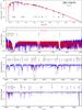 |
Fig. B.1 Upper panel: comparison between observed photometry (blue squares) and the flux-calibrated HST spectrum (blue line) with the SED of our best-fitting model (red line). Lower panels: comparison between observed normalized HST and HARPS spectra (blue solid line) and the best-fitting model (red dotted line). Hα is shown separately (see Fig. 3). |
All Tables
X-ray spectral parameters derived from the XMM-Newton observations of HD 54879 assuming a three-temperature plasma model.
Compilation of optical observations and measured Hα equivalent widths for HD 54879.
All Figures
|
Fig. 1 A schematic sketch of a star with a global dipole magnetic field, illustrating the formation regions of different features in the spectrum of HD 54879. Region I: blue-shifted UV resonance line absorption (e.g., C iv, Si iv); Region II: UV resonance line emission; Region III: shocked, X-ray emitting region; Region IV: recombination line emission at the magnetic equator (Hα, Hβ). |
| In the text | |
|
Fig. 2 The three HARPS observations focusing on Hα (upper panel) and a few photospheric lines (lower panel). |
| In the text | |
|
Fig. 3 Our best fitting model with parameters as in Table 1 (red dotted line) compared to the first four Balmer lines, as observed in the HARPS spectrum (blue solid line). The disk emission of Hα and Hβ is not included in the model. |
| In the text | |
 |
Fig. 4 Same as Fig. 3, but for several He i, ii lines. |
| In the text | |
|
Fig. 5 Selected CNO spectral lines of our best fitting model convolved with rotation profiles for vsini = 0,4, and 8 km s-1 (red, green, and black dotted lines, respectively), compared to observations (blue solid line). |
| In the text | |
|
Fig. 6 Comparison of normalized HST observations of the prototypical O9.7 V star HD 36512 (ID: 13346, PI: Ayres, pink solid line) and of HD 54879 (blue solid line) in Doppler space. Shown are the resonance lines C iv λλ1548,1551 (left panel) and Si iv λλ1394,1403 (right panel). |
| In the text | |
|
Fig. 7 Normalized HST observations of HD 54879 (blue solid line) compared to synthetic spectra with a terminal velocity of v∞ = 900 km s-1 and different mass-loss rates (given in the legend in [M⊙ yr-1]). |
| In the text | |
|
Fig. 8 Normalized HST observations of HD 54879 (blue solid line) compared to our best-fitting model, which accounts for a large microturbulence and superionization by X-rays. |
| In the text | |
|
Fig. 9 Normalized HST observations of HD 54879 (blue solid line) compared to our best-fitting model (red dotted line) and to the same model without the inclusion of X-rays (black dashed line). |
| In the text | |
|
Fig. 10 XMM-Newton PN, MOS1, and MOS2 spectra of HD 54879 (black, red, and green curves, respectively) with error bars corresponding to 3σ with the best fit three-temperature thermal model (solid lines). The model parameters are shown in Table 1. |
| In the text | |
|
Fig. 11 ASAS3 light curve of HD 54879. |
| In the text | |
|
Fig. 12 FEROS, FIES, and HARPS spectra of Hα taken in the years 2009–2015 (see legend and Table A.1). |
| In the text | |
|
Fig. 13 A few amateur SPO spectra of Hα, shown with a single HARPS spectrum for comparison. |
| In the text | |
|
Fig. 14 Equivalent widths of Hα versus heliocentric Julian date, as measured in the IACOB/OWN, HARPS and amateur SPO spectra. |
| In the text | |
|
Fig. B.1 Upper panel: comparison between observed photometry (blue squares) and the flux-calibrated HST spectrum (blue line) with the SED of our best-fitting model (red line). Lower panels: comparison between observed normalized HST and HARPS spectra (blue solid line) and the best-fitting model (red dotted line). Hα is shown separately (see Fig. 3). |
| In the text | |
Current usage metrics show cumulative count of Article Views (full-text article views including HTML views, PDF and ePub downloads, according to the available data) and Abstracts Views on Vision4Press platform.
Data correspond to usage on the plateform after 2015. The current usage metrics is available 48-96 hours after online publication and is updated daily on week days.
Initial download of the metrics may take a while.