| Issue |
A&A
Volume 606, October 2017
|
|
|---|---|---|
| Article Number | A41 | |
| Number of page(s) | 8 | |
| Section | Numerical methods and codes | |
| DOI | https://doi.org/10.1051/0004-6361/201731257 | |
| Published online | 05 October 2017 | |
The NOD3 software package: A graphical user interface-supported reduction package for single-dish radio continuum and polarisation observations
Max-Planck-Institut für Radioastronomie, Auf dem Hügel 69, 53121 Bonn, Germany
e-mail: This email address is being protected from spambots. You need JavaScript enabled to view it.
Received: 29 May 2017
Accepted: 13 July 2017
Abstract
Context. The venerable NOD2 data reduction software package for single-dish radio continuum observations, which was developed for use at the 100-m Effelsberg radio telescope, has been successfully applied over many decades. Modern computing facilities, however, call for a new design.
Aims. We aim to develop an interactive software tool with a graphical user interface for the reduction of single-dish radio continuum maps. We make a special effort to reduce the distortions along the scanning direction (scanning effects) by combining maps scanned in orthogonal directions or dual- or multiple-horn observations that need to be processed in a restoration procedure. The package should also process polarisation data and offer the possibility to include special tasks written by the individual user.
Methods. Based on the ideas of the NOD2 package we developed NOD3, which includes all necessary tasks from the raw maps to the final maps in total intensity and linear polarisation. Furthermore, plot routines and several methods for map analysis are available. The NOD3 package is written in Python, which allows the extension of the package via additional tasks. The required data format for the input maps is FITS.
Results. The NOD3 package is a sophisticated tool to process and analyse maps from single-dish observations that are affected by scanning effects from clouds, receiver instabilities, or radio-frequency interference. The “basket-weaving” tool combines orthogonally scanned maps into a final map that is almost free of scanning effects. The new restoration tool for dual-beam observations reduces the noise by a factor of about two compared to the NOD2 version. Combining single-dish with interferometer data in the map plane ensures the full recovery of the total flux density.
Conclusions. This software package is available under the open source license GPL for free use at other single-dish radio telescopes of the astronomical community. The NOD3 package is designed to be extendable to multi-channel data represented by data cubes in Stokes I, Q, and U.
Key words: methods: data analysis / techniques: image processing / techniques: polarimetric / radio continuum: general
© ESO, 2017
1. Introduction
Radio continuum and polarisation data from the 100-m Effelsberg radio telescope have usually been reduced and analysed with the NOD2 reduction system (Haslam 1974) and the library of routines described in the Hitch-Hiker’s Guide to NOD2 (Andernach 1985). The programs were written in Fortran and the maps needed to be in a special NOD2 data format. Several procedures were developed within NOD2 to reduce the so-called scanning effects.
Scanning effects in single maps can be suppressed with “presse” (Sofue & Reich 1979). Maps observed with multi-horn receivers can be combined with a restoration software (Emerson et al. 1979). Maps of observations scanned along different orientations within the sky can be combined with “basket weaving” (method unpublished) for orthogonally scanned maps or “plait” for double- or multi-horn observations (Emerson & Gräve 1988).
Present-day computing facilities offer interactive usage and graphical displays, fast data processing, and huge data storage. We designed an interactive software package for single-dish radio continuum observations, based on the FITS format, named NOD3, with a graphical user interface (GUI) that includes all tasks to produce final maps in total intensity and linear polarisation. Several of the data reduction methods originally introduced by NOD2 were significantly improved or revised.
While the widely used Common Astronomy Software Applications (CASA) package (McMullin et al. 2007) is mainly designed for the reduction and analysis of interferometer data, the new NOD3 package is – similar to its precursor NOD2 – explicitly developed for the different requirements of single-dish radio continuum observations.
2. Data format and general features
In order to make the new software package, NOD3, as flexible and compatible as possible with observations from other telescopes we chose the Flexible Image Transport System (FITS) format as the data format for the input maps. We labeled the header parameters of the FITS format identical to those chosen in CASA (McMullin et al. 2007). Additional header information can easily be added.
The program package is written in Python, which comfortably allows the user the inclusion of special tasks written by the individual user. In contrast to NOD2, the astronomical data in NOD3 are represented as a two-dimensional array or as a data cube for multi-channel observations, one each in Stokes I, Q, and U with its own header parameters.
The input parameters for all tasks can be entered either with the cursor or directly by typing the value. These parameters are shown and also stored within the tasks for the next application. They are also automatically compiled in a logfile that can easily be used to generate scripts for future utilisation and also for sequences (scripts) of different tasks. All tasks that have been applied to a map are listed in the NOD3 history file following the FITS header.
3. Typical data reduction steps for single-dish observations
The data stream (time series) from a telescope needs to be transformed into a two-dimensional map. We recommend the following steps:
-
Filtering of radio-frequency interference (RFI) in the raw continuum data stream from the output channels of the polarimeter (Stokes I, Q, U for each horn).
-
Calibration of the Stokes parameters (I, U, Q) by applying the MuellerMatrix.
-
Interpolation of the raw data with a sinc weighting function into square pixels and combination into maps in FITS format.
-
For maps scanned in azimuth direction, generate two additional maps for the sidereal time and the parallactic angle for each pixel in the map, to allow the transformation from the horizontal coordinate system to the equatorial coordinate system, if necessary.
For each radio telescope a specific system for generating the raw data has been developed. Those of the 100-m Effelsberg telescope are preprocessed with the “Toolbox” package (see Appendix). The format of the raw data from multi-horn Effelsberg observations is set in a way that all maps (Stokes I, U, Q) of a single coverage of a target are stored in one file, together with two additional maps for the sidereal time and parallactic angle for each pixel in the map.
The NOD3 package includes all necessary steps for the reduction of the raw FITS maps to the final maps. First, it is necessary to correct the base levels and suppress the scanning effects. These scanning effects can be further reduced by the following reduction steps:
-
combination of maps (for each channel) from multi-hornobservations;
-
averaging of the maps of total intensity channels to a map in Stokes I;
-
combination of all single coverages to maps in Stokes I, Q, and U;
-
computation of maps of linearly polarised intensity PI (bias-corrected) and polarisation angle PA;
-
calibration of absolute flux density with help of a map of a calibration source;
-
checking and correction of absolute polarisation angle with the help of a map of a linearly polarised calibration source.
4. Improved methods
Although we kept the original ideas of the reduction routines from the NOD2 library, we refined the methods if possible (e.g. Flatten) and also introduced some new procedures (e.g. Restore). As a result, we are able to reduce the scanning effects, which are distortions in the direction along which the map area was scanned on the sky during the observations. Furthermore, we can significantly reduce the root mean square (rms) noise in the maps.
4.1. Removal of scanning effects, base level correction, and noise reduction
4.1.1. Base level correction: Adjust
The measured system temperature of the receiver not only contains astronomical signals but also contains atmospheric and ground radiation. The latter depends on the elevation of the telescope and is usually much larger than the astronomical signal. The base level can be corrected for by a polynomial fit to each scan of a map. For small scanning lengths (<1°) it is sufficient to correct the base level linearly, otherwise the fit can have a higher order.
In principle we do not know the absolute base level of a map. Hence, we have to adjust the base level relative to zero at the beginning and at the end of each scan. To achieve this, we select a range of points on each side of each scan over which we determine the base level by a median filter. Although we get different median values for each scan, we get smooth transitions to adjacent scans owing to the application of the median filter. The advantage of the median filter is that it excludes extrema caused by point sources or RFI. Base levels can be affected by compact astronomical sources at the beginning or end of a scan, which is avoided with our filtering method. If scanning effects still remain, other methods are required; see e.g. Sect. 4.1.2.
4.1.2. Suppressing of scanning effects: Flatten
Because of several kinds of scanning effects (i.e. weather, atmospheric or ground radiation, and receiver instabilities) an individual single map usually still includes scanning effects after adjusting the scans to a zero level. It is possible to reduce these distortions with the method of “unsharp masking” (Sofue & Reich 1979). In contrast to that method, we do not smooth the data to values larger than the beam width of the telescope along the scanning direction and only slightly perpendicular to the scanning direction1 by 1.5 times the scan separation; this ensures that astronomical structures are not affected. The difference between the original and smoothed map is taken to fit a polynomial baseline iteratively. An acceptable result is reached after a few iterations, for which fits of the order 3 or higher can be applied if necessary.
4.1.3. Single-horn observations: BasketWeaving
This task can be used to remove scanning effects in maps that are scanned at least once along two orthogonal directions (in astronomical coordinates). Clouds moving in the atmosphere cause a time-dependent base level, which shows up as scanning effects. Base level distortions due to atmospheric or ground radiation cannot be removed and can only be suppressed by averaging. If more than one coverage is available in each scanning direction, all maps with the same scanning direction are averaged first.
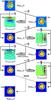 |
Fig. 1 Showing the work flow of the basket-weaving procedure, based on observations of the Tycho supernova remnant at 4.85 GHz with the Effelsberg 100-m telescope. The sketch shows 2 iterations of the method. |
The BasketWeaving algorithm is illustrated in Fig. 1. The goal is to remove the scanning effects by iteratively forming difference maps between the two orthogonal maps, starting with the input maps MapL,0(l,b) and MapB,0(l,b) (panels 1 and 2 of Fig. 1, respectively),  (1)This should remove the astronomical signal completely, except in case of pointing errors. Next, the global rms value of the difference map is calculated and all map values greater in magnitude than ± σclip × rms, where σclip is a user-given input, are set to this value. To ensure that no astronomical signal is left in the difference map, this cycle of rms computation and clipping is iterated three times. Each row of the clipped difference map is then smoothed by a (one-dimensional) Hanning window of width corresponding to half the column or row length, and the smoothed map (Fig. 1, panel 3) is subtracted from the original (averaged) map in the according scanning direction
  (2)The resulting map (panel 4), in turn, is now subtracted from the original (averaged) map in the other scanning direction
  (3)and the above steps (clipping, smoothing, and subtraction of the smoothed map) are repeated, but this time the Hanning smoothing is performed for each column (panels 5 and 6), i.e.
  (4)The entire process is iterated for successively narrower smoothing windows, hence higher spatial frequencies, until a minimum window size is reached. We choose a step size of four pixels and a minimum window size of five pixels, but these values are not critical.
In a final step (panel 11), the program forms the average of the last maps obtained in the two orthogonal scanning directions, which should be “cleaned” from scanning effects on various length scales,  (5)This BasketWeaving method is effective even for a pair of orthogonally scanned maps.
4.1.4. Restoration of dual- or multiple-horn observations: Restore
Dual- or multiple-horn observations can reduce scanning effects significantly. If the horns are mounted parallel to the azimuth direction and the telescope covers the field of the sky with azimuth scans, the assumption is that the horns detect the same clouds but at different positions on the sky. Emerson et al. (1979) published a method to restore multiple-horn observations obtained with a single-dish radio telescope. This method has the disadvantage that the noise increases with the number of pixels along a scan, which was noted already by Emerson et al. (1979). The method uses the difference of two maps covered by different horns with the underlying idea that the weather effects disappear while the astronomical signal remains in difference, shifted by the horn separation.
The new method takes a different approach by shifting the related scans of two horns by their azimuth distance. In this case, when computing the difference map, the astronomical signal disappears but the scanning effects due to the weather are now seen in difference. So we can manipulate the difference map without running the risk of influencing the astronomical signal.
If x is the astronomical position (measured in azimuth) at the sky and h is the distance in azimuth of two horns H1 and H2, then ![Mathematical equation: \begin{equation} D(x) = [H1(x+h/2) - H2(x-h/2)] / h , \end{equation}](/articles/aa/full_html/2017/10/aa31257-17/aa31257-17-eq23.png) (6)corresponds to a derivation of the signals of the two horns (Fig. 2), assuming equal weather effects in both horns. Now, an integration of the function D(x) solves the problem and we can easily restore the scanning (weather) effects W(a) at azimuth position a,
(6)corresponds to a derivation of the signals of the two horns (Fig. 2), assuming equal weather effects in both horns. Now, an integration of the function D(x) solves the problem and we can easily restore the scanning (weather) effects W(a) at azimuth position a,  (7)and subtract it from the corresponding scans from each of the horns. The integration constant c yields an offset, which has to be corrected separately with the Adjust method described in Sect. 4.1.1.
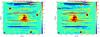 |
Fig. 2 One coverage of the spiral galaxy IC 342 observed at 4.85 GHz with the Effelsberg 100-m telescope (Beck 2015), simultaneously covered by the two different horns in the secondary focus. The maps from the two horns show an offset in source position, while the weather effects are at the same position. |
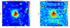 |
Fig. 3 Comparison of the results of the restoration process of the two maps shown in Fig. 2 after applying the NOD3 method (left) and NOD2 method (right). |
In our case h describes the distance of two horns. The value h is always greater than zero. For a mathematically correct treatment h → 0 is required. This acts like a low-pass filter and structures on scales smaller than the distance of the horns are not detectable. Small structures, however, are not relevant in our case, as we assumed that weather signals on small scales are equal in both horns, hence its angular extent is larger than that corresponding to the horn separation.
The low-pass filter has a positive effect as it avoids significant noise in the restored weather effects W(a) at azimuth position a. After subtracting W from the corresponding scans of the two horns, averaging of the scans leads to a noise improvement by a factor of  compared to that in single-horn observations, regardless of the length of the scan.
The noise levels in Fig. 3 are 14.7 units (left) and 29.3 units (right). So the signal-to-noise ratio of the new restoring method is two times better than for the old NOD2 method. The old NOD2 method increases the noise with the number of pixels per azimuth row. The new NOD3 method does not increase the noise but corrects the weather effects in each map separately, which yields an improvement in total of about a factor of 2.
Background sources at the edges of the scanned area do not influence the restoration process with the new method because only the overlapping areas are considered and hence do not have to be eliminated beforehand. This is different from the previous method of restoring double-horn observations by Emerson et al. (1979). Furthermore, the maps created with the new method do not suffer from a maximum visible structure of about three times the horn distance as was the case for the previous method by Emerson et al. (1979).
If a large number of coverages are combined, the final map created with the new method (Fig. 4 left) shows clear improvements compared to the map created with the previous method (Fig. 4 right). That is, the improvement in the noise level is a factor of 2, the background level is smoother, and fewer artefacts are visible at the edges. As a result, the diffuse emission of the galaxy can be traced to larger radii. A level of three times the rms noise is reached at 43′ radius compared to 35′ radius with the previous method (Beck 2015).
For observations with more than two horns, it is possible to combine all pairs of horns that are aligned in the azimuth scanning direction. However, the distance of the combined horns should not be too large, so that weather effects are similar in all horns and the low-pass filter effect is not too large.
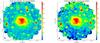 |
Fig. 4 Comparison of the results of the restoration process of all 20 coverages observed by Beck (2015) after the NOD3 method (left) and NOD2 method (right). |
4.2. Polarisation: PolInt
Polarised radio emission comes as Stokes Q and U maps. Both contain receiver noise NQ,U,P that is not part of the astronomical signal. The noise shifts the observed polarised intensity  up with respect to the “true” polarised intensity PT, which is called the polarisation bias.
The difference  has the probability density known as the Ricedistribution, which is always positive definite. The bias effect becomes more significant for smaller signal to noise of QT and UT. Rewriting the above formula to
 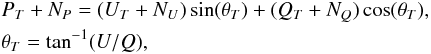 (8)allows us to get rid of the bias. The method is described comprehensively by Müller et al. (2017). It requires the knowledge of the “true” angle θT from the “true” QT and UT. A good approximation is given by the “modified median filter” of the adjacent angles in the map as described in Müller et al. (2017).
In most cases we have just Q and U and need to build the modified median value θm of the adjacent angles, 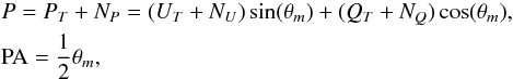 (9)where PA is close to the “true” polarisation angle. Numerical simulations show that P is almost bias free and the probability density of the noise NP is Gaussian with the same standard deviation as those of NQ and NU. The noise distribution of NQ and NU does not have to be Gaussian but needs to be centred around zero.
4.3. Combination of single-dish with interferometer observations: Immerge
It is a well-known problem that large holes in the u, v plane of interferometric data causes “missing flux” because telescope arrays do not cover all short baselines. This missing flux can be added from a large single-dish such as the Effelsberg 100-m radio telescope. Ideally, the receiver frequencies should cover the same range at both observations. Instead of combining both maps in the Fourier plane as in AIPS (Greisen 2003) or CASA (McMullin et al. 2007), we propose a straightforward combination method in the image plane. The resulting map is similar to the result of “feathering” in CASA.
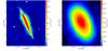 |
Fig. 5 VLA map (left) of the edge-on galaxy NGC 891. The map shows a missing flux that can be filled in with a single-dish Effelsberg map (right; Schmidt et al., in prep.). |
The single-dish map has to be resampled to the pixel resolution of the interferometer map and the interferometer map has to be convolved to the angular resolution of the single-dish map. The difference of both maps gives the missing flux of the interferometer map with the angular resolution of the single-dish map. In order to add the difference map to the interferometer map it is necessary to deconvolve the difference map to the resolution of the interferometer map.
The spatial structure of the difference map contains no structures smaller than the resolution of the single-dish map. Given that there is an overlap in the spacial frequency range between the single-dish and interferometer maps, the error should be small if we approximate the deconvolution by simply rescaling the difference map with the ratio of their beam areas Ω, ![Mathematical equation: \begin{eqnarray} D(l, b) &=& SD(l, b) - I(l, b) ,\nonumber\\ d(l, b) &=& [\Omega_{\rm I}/\Omega_{\rm SD}] \cdot D(l, b) ,\nonumber\\ \hat{I}(l, b) &=& I(l, b) + d(l, b) , \end{eqnarray}](/articles/aa/full_html/2017/10/aa31257-17/aa31257-17-eq51.png) (10)where D(l,b) is the difference map between the single-dish map SD(l,b) and the interferometer map I(l,b) with their beam areas ΩI and ΩSD. The rescaled map d(l,b) can now be added to the interferometer map I(l,b).
(10)where D(l,b) is the difference map between the single-dish map SD(l,b) and the interferometer map I(l,b) with their beam areas ΩI and ΩSD. The rescaled map d(l,b) can now be added to the interferometer map I(l,b).
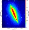 |
Fig. 6 Combination of the VLA map and Effelsberg maps of NGC 891 (Schmidt et al., in prep.). |
The advantage of this method is that the missing flux can be determined directly from the difference of the two maps in the image domain.
4.4. Box integration of edge-on galaxies: BoxModels
The determination of the vertical scale heights of the total radio continuum intensity of spiral galaxies seen edge-on (applicable for galaxy inclinations > 80°) goes back to the method initially described and applied by Dumke et al. (1995). The task is called “BoxModels” and works with (total intensity) maps in FITS format smoothed to a circular beam.
Within the task, strips are defined as perpendicular to the major axis of the galaxy (called the z-direction) by giving its position angle. The width and lengths of each strip can be defined with respect to the central position of the galaxy. Within one strip, the number and width of boxes can be chosen wherein the radio intensities are averaged. As errors of these values the noise errors within one box can be taken. The better way is to take the standard deviation of the mean in each box. In order to exclude the expected intensity gradient in the z-direction, the standard deviation is calculated along each rows parallel to the major axis of the galaxy separately within each box. Finally, they are averaged over all rows within each box. These averaged intensity distributions along each strip are used to fit the vertical radio scale height (along each single strip).
For inclinations i< 90°, the observed intensity distribution is the superposition of the intrinsic vertical distribution of the disk and halo emission and the inclined disk emission (even for an infinitesimally thin disk), convolved with the telescope beam. Because we are only interested in the vertical intensity distribution, the observed distribution has to be corrected for the contribution of the disk, which depends only on the diameter of the disk and its inclination.
We approximately compensate the projection of the inclined galaxy with an increase of the beam width perpendicular to its disk by ΔHPBW = Rcos(r/R·π/ 2)cosi, where HPBW is the half power beam width, R is the radius of the galaxy, r the distance from the centre, and i its inclination. Then the effective  . The resulting distribution is still Gaussian in the vertical direction with
 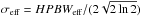 , decreasing from the centre outwards along the major axis of the galaxy towards the telescope beam width HPBW at the edges.
As an exact deconvolution of the observed intensity distribution with HPBWeff cannot be applied, we assume different possible vertical distributions convolved with the corresponding HPBWeff for each strip and compare these with the observed distributions by least-squares fits. Similar to Dumke et al. (1995), an intrinsic exponential 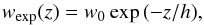 (11)or an intrinsic Gaussian distribution
  (12)is assumed with peak intensity w0 and scale height h. This is convolved with the effective telescope beam
 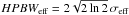 ,
,  (13)which describes the contribution of the telescope beam and the projected emission of the infinitesimally thin disk. The convolved emission profile has the form
 ![Mathematical equation: \begin{eqnarray} \label{convexp} W_{\mathrm{exp}}(z)&=&\frac{w_{0}}{2}\exp{\left(-z^{2}/2\sigma_{\rm eff}^{2}\right)} \nonumber\\[1.5mm] &&\quad \times\left[\exp{\left(\frac{\sigma_{\rm eff}^{2}-zh}{\sqrt{2}\sigma_{\rm eff} h} \right)}^{2}\mathrm{erfc}\left(\frac{\sigma_{\rm eff}^{2}-zh} {\sqrt{2}\sigma_{\rm eff} h}\right)\right. \nonumber\\[1.5mm] &&\left.\quad+ \exp{\left(\frac{\sigma_{\rm eff}^{2}+zh}{\sqrt{2}\sigma_{\rm eff} h} \right)}^{2}\mathrm{erfc}\left(\frac{\sigma_{\rm eff}^{2}+zh} {\sqrt{2}\sigma_{\rm eff} h}\right)\right], \end{eqnarray}](/articles/aa/full_html/2017/10/aa31257-17/aa31257-17-eq74.png) (14)in case of an exponential intrinsic distribution (Sievers 1988), where erfc is the complementary error function, defined as
(14)in case of an exponential intrinsic distribution (Sievers 1988), where erfc is the complementary error function, defined as  (15)For a Gaussian intrinsic distribution, the convolution yields (Dumke 1994)
  (16)The vertical radio scale heights h can be determined by fitting one or two “convolved” exponential or Gaussian functions of the form given in Eqs. (14) or (16) to the averaged radio intensities along each strip of a galaxy. The least-squares fits are made using the Levenberg−Marquard method. Single boxes along a strip with mean values that are smaller than the rms-noise intensity level of the map are omitted by the fitting procedure. The quality of the fit along each strip is determined by a reduced χ2-test.
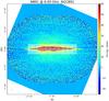 |
Fig. 7 Combination of the VLA and Effelsberg maps, rotated by the position angle and boxes indicated. |
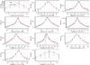 |
Fig. 8 For each individual strip along the major axis a profile is created from which a two-component scale-height model is fitted. |
4.5. Integration of galaxy segments in face-on view
In addition to the integration within boxes (as decribed above) and elliptical rings, NOD3 also offers the possibility to integrate map values in equally sized segments of rings that are circular in the plane of the galaxy. The primary application of this is to study different regions of spiral galaxies in a face-on view even if they are inclined. For this purpose, the task first rotates the input map by a user-given position angle and then deprojects the map by the specified inclination angle of the galaxy, so that it appears face-on. This is possible for inclinations up to 80°.
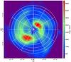 |
Fig. 9 Example of a sectored target. |
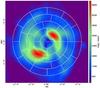 |
Fig. 10 Example of a segmented target. |
The integrated and averaged values are then computed for each segment in a set of concentric rings, where the number of rings (up to 15), the number of segments (up to 180 per ring), and the maximum ring radius are selected by the user. For the arrangement of the ring segments, two different options are offered. (i) In sector mode, all rings are divided into an equal number of segments with a constant separation in azimuth, in which case the width of the rings decreases with radius (Fig. 9). (ii) In segment mode, all rings have the same width, so that the number of segments per ring increases with radius (Fig. 10).
5. Summary
The NOD3 program package is designed to reduce and analyse single-dish maps. It is the result of developing an
interactive software package with a GUI that includes all the necessary programs to obtain the final maps in total intensity and linear polarisation. The program package is written in Python. The required data format for the input maps is FITS. The NOD3 package is especially powerful to remove “scanning effects” due to clouds, receiver instabilities, or RFI in single-dish observations. We significantly improved or revised several of the data reduction methods introduced by NOD2. The “basket-weaving” tool combines orthogonally scanned maps to a final map that is almost free of scanning effects. The new restoration tool for dual-beam observations reduces the noise by a factor of about two. The combination of single-dish with interferometer data in the map plane ensures the recovery of the full flux density. The NOD3 package also offers an improved method for bias correction of the polarised intensity map (Müller et al. 2017), and it offers the possibility of including special tasks written by the individual observer.
The NOD3 package is designed to be extendable to multi-channel data represented by data cubes in Stokes I, Q, and U, which is planned as the next step of our work. Another future extension will be the cleaning of the telescope side lobes.
The NOD3 software package is available under the open source license GPL for a free use at other single-dish radio telescopes of the astronomical community. The latest version can be obtained at the gitlab server of MPIfR Bonn2. A NOD3 user manual is included and available from the gitlab at the MPIfR Bonn.
According to the sampling theorem, the separation between scans must be smaller than half the beam width.
Acknowledgments
We thank René Gießübel, Maja Kierdorf, and Carolina Mora for testing the program package, René Gießübel for his work on the NOD3 User Manual, and Uli Klein for fruitful discussions. We also thank Alexander Kraus for critical comments on the manuscript.
References
- Andernach, H. 1985, Hitch-Hiker’s Guide to NOD2, MPIfR, Bonn [Google Scholar]
- Beck, R. 2015, A&A, 578, A93 [NASA ADS] [CrossRef] [EDP Sciences] [Google Scholar]
- Dumke, M. 1994, Diploma Thesis, University of Bonn [Google Scholar]
- Dumke, M., Krause, M., Wielebinsky, R., & Klein, U. 1995, A&A, 302, 691 [NASA ADS] [Google Scholar]
- Emerson, D. T., & Gräve, R. 1988, A&A, 190, 353 [NASA ADS] [Google Scholar]
- Emerson, D. T., Klein, U., & Haslam, C. G. T. 1979, A&A, 76, 92 [NASA ADS] [Google Scholar]
- Haslam, C. G. T. 1974, A&AS, 15, 133 [Google Scholar]
- Greisen, E. W. 2003, in Information Handling in Astronomy – Historical Vistas, ed. A. Heck (Dordrecht: Kluwer), 109 [Google Scholar]
- McMullin, J. P., Waters, B., Schiebel, D. et al. 2007, Astronomical Data Analysis Software and Systems XVI eds. R. A. Shaw, F. Hill, & D. J. Bell (San Francisco, CA: ASP), ASP Conf. Ser., 376, 127 [Google Scholar]
- Muders, D., Polehampton, E., & Hatchell, J. 2005, Multi-beam FITS Raw Data Format, APEX Report APEX-MPI-IFD-0002, Rev. 1.57 [Google Scholar]
- Müller, P., Beck, R., & Krause, M. 2017, A&A, 600, A63 [NASA ADS] [CrossRef] [EDP Sciences] [Google Scholar]
- Sieber, W., Haslam, C. G. T., & Salter, C. J. 1979, A&A, 74, 361 [NASA ADS] [Google Scholar]
- Sievers, A. 1988, Ph.D. Thesis, University of Bonn [Google Scholar]
- Sofue, Y., & Reich, W. 1979, A&AS, 38, 251 [NASA ADS] [Google Scholar]
Appendix A: Toolbox: The pre-processing software at the Bonn 100-m Telescope
The data observed in the mapping mode (“on the fly”) with the Effelsberg 100-m telescope are stored as they are received from the backends together with telescope position information and their time stamps. This is necessary to link astronomical coordinates and flux intensities. The mapping mode allows coverage of an arbitrarily chosen area on the sky that is measured in astronomical coordinates. The coverage can be scanned along the longitude axis or latitude axis in any coordinate system. The non-scanning coordinate is always fixed for one scan. With the following scans the non-scanning coordinate is incremented usually by a third of the telescope beam width (sampling theorem).
All frontends and backends at the 100-m radio telescope at Effelsberg are steered by uniform blank and sync signals produced by hardware. A blank-sync generator is designed to produce short time signals interrupted by a blank time signal. After n blank time signals a sync time signal is sent that contains the information of the integration time between the blank time signals. The length of a sync time signal is called phasetime, i.e.
the integration time of one phase. The blank time is dead time while the measurement is not recording. The blank time is much smaller then the sync time. Within one phase a noise diode or any other signal could switch alternately on and off to the frontend. We call a successive series of same phases phasecycle. A phasecycle is used for a pre-reduction in order to calibrate the astronomical signals.
Each phase is written to disk in the MBFITS format (Muders et al. 2005) during the observations. This data is used by a dedicated preprocessing software called Toolbox, which, similar to NOD3, is completely written in Python. The MBFITS files are used as input for the Toolbox. All radio continuum and spectral polarimeter data are pre-reduced by the Toolbox. Preprocessing means mainly calibrating the astronomical signals by the signal of noise diode (calsignal) removing radio frequency interference RFI, pre-adjusting the baselines, preparing, and calibrating the polarisation data.
The Toolbox is also used for the analysis of, for example cross-scans over a point-like source, on-offs, or skydips. In the case of sky mapping, the Toolbox outputs a FITS file ready for the NOD3 software.
All Figures
|
Fig. 1 Showing the work flow of the basket-weaving procedure, based on observations of the Tycho supernova remnant at 4.85 GHz with the Effelsberg 100-m telescope. The sketch shows 2 iterations of the method. |
| In the text | |
|
Fig. 2 One coverage of the spiral galaxy IC 342 observed at 4.85 GHz with the Effelsberg 100-m telescope (Beck 2015), simultaneously covered by the two different horns in the secondary focus. The maps from the two horns show an offset in source position, while the weather effects are at the same position. |
| In the text | |
|
Fig. 3 Comparison of the results of the restoration process of the two maps shown in Fig. 2 after applying the NOD3 method (left) and NOD2 method (right). |
| In the text | |
|
Fig. 4 Comparison of the results of the restoration process of all 20 coverages observed by Beck (2015) after the NOD3 method (left) and NOD2 method (right). |
| In the text | |
|
Fig. 5 VLA map (left) of the edge-on galaxy NGC 891. The map shows a missing flux that can be filled in with a single-dish Effelsberg map (right; Schmidt et al., in prep.). |
| In the text | |
|
Fig. 6 Combination of the VLA map and Effelsberg maps of NGC 891 (Schmidt et al., in prep.). |
| In the text | |
|
Fig. 7 Combination of the VLA and Effelsberg maps, rotated by the position angle and boxes indicated. |
| In the text | |
|
Fig. 8 For each individual strip along the major axis a profile is created from which a two-component scale-height model is fitted. |
| In the text | |
|
Fig. 9 Example of a sectored target. |
| In the text | |
|
Fig. 10 Example of a segmented target. |
| In the text | |
Current usage metrics show cumulative count of Article Views (full-text article views including HTML views, PDF and ePub downloads, according to the available data) and Abstracts Views on Vision4Press platform.
Data correspond to usage on the plateform after 2015. The current usage metrics is available 48-96 hours after online publication and is updated daily on week days.
Initial download of the metrics may take a while.