| Issue |
A&A
Volume 606, October 2017
|
|
|---|---|---|
| Article Number | A14 | |
| Number of page(s) | 18 | |
| Section | Galactic structure, stellar clusters and populations | |
| DOI | https://doi.org/10.1051/0004-6361/201731142 | |
| Published online | 26 September 2017 | |
Binary companions of nearby supernova remnants found with Gaia
1 Institute of Astronomy, University of Cambridge, Madingley Rise, Cambridge, CB3 0HA, UK
e-mail: This email address is being protected from spambots. You need JavaScript enabled to view it.
2 School of Physics, O’Brien Centre for Science North, University College Dublin, Belfield, Dublin 4, Ireland
3 Astrophysics Group, Cavendish Laboratory, 19 J. J. Thomson Avenue, Cambridge CB3 0HE, UK
Received: 9 May 2017
Accepted: 3 July 2017
Abstract
Aims. We search for runaway former companions of the progenitors of nearby Galactic core-collapse supernova remnants (SNRs) in the Tycho-Gaia astrometric solution (TGAS).
Methods. We look for candidates among a sample of ten SNRs with distances ≲2kpc, taking astrometry and G magnitude from TGAS and B,V magnitudes from the AAVSO Photometric All-Sky Survey (APASS). A simple method of tracking back stars and finding the closest point to the SNR centre is shown to have several failings when ranking candidates. In particular, it neglects our expectation that massive stars preferentially have massive companions. We evolve a grid of binary stars to exploit these covariances in the distribution of runaway star properties in colour – magnitude – ejection velocity space. We construct an analytic model which predicts the properties of a runaway star, in which the model parameters are the location in the grid of progenitor binaries and the properties of the SNR. Using nested sampling we calculate the Bayesian evidence for each candidate to be the runaway and simultaneously constrain the properties of that runaway and of the SNR itself.
Results. We identify four likely runaway companions of the Cygnus Loop (G074.0−08.5), HB 21 (G089.0+ 04.7), S147 (G180.0+ 01.7) and the Monoceros Loop (G205.5+ 00.5). HD 37424 has previously been suggested as the companion of S147, however the other three stars are new candidates. The favoured companion of HB 21 is the Be star BD+50 3188 whose emission-line features could be explained by pre-supernova mass transfer from the primary. There is a small probability that the 2M⊙ candidate runaway TYC 2688-1556-1 associated with the Cygnus Loop is a hypervelocity star. If the Monoceros Loop is related to the on-going star formation in the Mon OB2 association, the progenitor of the Monoceros Loop is required to be more massive than 40M⊙ which is in tension with the posterior for our candidate runaway star HD 261393.
Key words: supernovae: general / binaries: close / ISM: supernova remnants / methods: statistical / stars: emission-line, Be
© ESO, 2017
1. Introduction
Supernovae (SNe) mark the deaths of stars. They can be divided into two broad categories: core-collapse SNe from the gravitationally powered explosion of massive stars (e.g. Smartt 2009), and Type Ia SNe from the thermonuclear destruction of white dwarfs (e.g. Hillebrandt & Niemeyer 2000). In both cases, there has been considerable interest in recent years in understanding their progenitor systems for reasons as diverse as testing stellar evolutionary models, improving their use as cosmological probes, and understanding their role in driving galactic evolution.
The most direct method for studying the progenitors of supernovae is to detect them in pre-explosion imaging. This is limited however to the handful of cases where SNe have exploded in a nearby galaxy with deep, high-resolution images. Furthermore, it is most suited for studying core-collapse supernova progenitors (Smartt 2009) which are luminous supergiants (although see Li et al. 2011a; and McCully et al. 2014, for applications to Type Ia SNe). Alternative techniques to infer core-collapse SN progenitor properties using nucleosynthetic yields from late-time spectroscopy of SNe (e.g. Jerkstrand et al. 2014), or hydrodynamic estimates of ejecta mass (Bersten et al. 2014) are always model dependent. For Type Ia SNe, the spectroscopic and photometric signatures of interaction between SN ejecta and a companion may be used to constrain the progenitor system, but are relatively weak effects (Maeda et al. 2014).
Another means to study SN progenitors is to search for their former binary companions that have survived the explosion. At least 70% of massive stars are seen to be in binary systems (e.g. Sana et al. 2012). Furthermore, in a handful of cases, a surviving binary companion has been detected in deep imaging of extragalactic core-collapse SNe (Maund & Smartt 2009; Folatelli et al. 2014). Type Ia SNe require a binary companion to explode (Hillebrandt & Niemeyer 2000), and may leave behind a detectable non-degenerate companion (e.g. Han 2008; Pan et al. 2014; Noda et al. 2016, and references therin). For both Type Ia and core-collapse SNe, the stellar parameters of a surviving binary companion can constrain the evolutionary status of the SN progenitor at the point of explosion (Maund & Smartt 2009; Bersten et al. 2012). A SN progenitor companion may also be polluted with metals from the explosion (Israelian et al. 1999, and more recently Liu et al. 2015).
Several searches have already been made for runaway stars in Galactic Type Ia SN remnants, most notably in Tycho’s SN where a possible candidate (designated Tycho G) has been claimed to be the former binary companion (Ruiz-Lapuente et al. 2004; González Hernández et al. 2009; Bedin et al. 2014). This association has since been disputed (Kerzendorf et al. 2009, 2013; Xue & Schaefer 2015). Searches within other Galactic remnants such as that of SN 1006 (González Hernández et al. 2012) and Kepler’s SN (Kerzendorf et al. 2014) have failed to yield a companion, while a non-degenerate companion has been almost completely ruled out for SNR 0509−67.5 in the Large Magellanic Cloud (Schaefer & Pagnotta 2012).
Searches for companions to core-collapse SNe have mostly focussed on runaway OB stars near SN remnants (Blaauw 1961; Guseinov et al. 2005). HD 37424, a main sequence B star, has been proposed to be associated with the SN remnant S147 (Dinçel et al. 2015). The pulsar PSR J0826+2637 has been suggested to share a common origin with the runaway supergiant G0 star HIP 13962 (Tetzlaff et al. 2014), although there is no identified SNR. In the Large Magellanic Cloud, the fastest rotating O-star (VFTS102) has been suggested to be a spun-up SN companion associated with the young pulsar PSR J0537−6910 (Dufton et al. 2011).
Recently Kochanek (2017) used Pan-STARRS1 photometry (Chambers et al. 2016), the Green et al. (2015) dust-map and the NOMAD (Zacharias et al. 2005) and HSOY (Altmann et al. 2017) proper motion catalogues to search for runaway former companions of the progenitors of the three most recent, local core-collapse SNe: the Crab, Cas A and SN 1987A. Based on a null detection of any reasonable candidates Kochanek (2017) put limits on the initial mass ratio q = M2/M1 ≲ 0.1 for the nominal progenitor binary of these SNRs. Kochanek (2017) note that this limit implies a 90% confidence upper limit on the q ≳ 0.1 binary fraction at death of fb< 44% in tension with observations of massive stars.
The reason to search for runaway companions of core-collapse supernovae is that their presence or absence can be used to constrain aspects of binary star evolution. These include mass transfer rates, common-envelope evolution and the period and binary fraction distributions. Runaway stars are interesting in their own right for their dynamical properties with the fastest runaway stars being unbound from the Milky Way.
In this work, we present a systematic search for SN-ejected binary companions within the Gaia Data Release 1 (DR1; Gaia Collaboration 2016b). Unfortunately, the Kepler SNR is too distant at around 6kpc to search for a companion using DR1, however ten other remnants including S147 lie within our distance cut-off of 2kpc. The data sources for both the runaways and the SNR are discussed in Sect. 2. We then outline two approaches to this problem – the first using purely kinematic methods in Sect. 3, the second exploiting colour, magnitude and reddening together with the peculiar velocity of the progenitor binary with a Bayesian framework in Sect. 4. For four SNRs (the Cygnus Loop, HB 21, S147 and the Monoceros Loop) we identify likely runaway companions which are discussed in detail in Sect. 5.
2. Sources of data
The list of candidate stellar companions for each SNR is taken from a cross-match of TGAS and APASS (Sect. 2.1). There is no analogously uniform catalogue for SNRs and so we conduct a literature review for each SNR to establish plausible estimates for the central position, distance and diameter, which we discuss in Sect. 2.2 and in Appendix A.
2.1. Summary of stellar data
On the 14th September 2016 the Gaia Data Release 1 (GDR1) was made publicly available (Gaia Collaboration 2016a,b). The primary astrometric component of the release was the realisation of the Tycho-Gaia astrometric solution (TGAS), theoretically developed by Michalik et al. (2015), which provides positions, parallaxes and proper motions for the stars in common between the GDR1 and Tycho-2 catalogues. At 1kpc the errors in the parallax from TGAS typically exceed 30%. To constrain the distance of the candidates we nearest-neighbour cross-match with the AAVSO Photometric All-Sky Survey (APASS) DR9 to obtain the B−V colour. Gaia Data Release 2 is anticipated in early 2018 and will contain the additional blue GBP and red GRP magnitudes. Substituting for B−V with the GBP−GRP colour will allow our method to be applied using only data from Gaia DR2.
2.2. Summary of individual SNRs
We select SNRs that are closer than 2kpc, having stars in our TGAS-APASS cross-match within the central 25% of the SNR by radius, and lying within the footprint of Pan-STARRS so we can use the 3D dustmap of Green et al. (2015). The SNRs in our sample are typically older than 10kyr and so will have swept up more mass from the ISM than was ejected, which makes it difficult to type them from observations of their ejecta. We can say that these SNRs are likely the remnants of core-collapse SNe since around 80% of Galactic SNe are expected to be core-collapse SNe (e.g. Mannucci et al. 2005; Li et al. 2011b). Moreover, several are identified with regions of recent star formation (i.e. G205.5+ 00.5 with Mon OB2) or molecular clouds in OB associations (i.e. G089.0+ 04.7 with molecular clouds in Cyg OB7). The properties of this sample of ten SNRs are given in Table 1, where NTGAS is the number of candidates found in TGAS and NTGAS + APASS is the number remaining after the cross-match with APASS.
Establishing a potential association between a star and a SNR requires us to demonstrate a spatial coincidence at around the time of the supernova explosion. The relevant properties of each SNR are then the location of the centre (α,δ)SNR, distance dSNR, age tSNR, angular diameter θSNR and either the proper motion (μα ∗,μδ)SNR or peculiar velocity (vR,vz,vφ)SNR.
We take the Ferrand & Safi-Harb (2012, known as SNRcat and Green (2014) catalogues as the primary sources of SNR properties. We use the positions and angular diameters from the detailed version of the Green catalogue that is available online1. The distance to a SNR is usually uncertain and so we describe the origin of each distance in Appendix A.
We do not use estimates of the ages of SNRs because distance estimates to SNRs are degenerate with the age, so these two measurements are not independent. We thus conservatively assume that the supernova must be older than 1kyr and younger than 150kyr. A younger supernova at 1kpc would very likely be in the historical record (Stephenson & Green 2002; Green & Stephenson 2003) and the shell of an older SNR would no longer be detectable.
Determining the location of the centre of a SNR is usually not straightforward. The standard method to obtain the centre is to calculate the centroid of the projected structure of the SNR shell on the sky, but this position can be obfuscated by various effects such as the interaction between the ejecta and the local ISM, overlap between SNRs, and background objects misclassified as belonging to the SNR. G074.0−08.5 (Cygnus Loop) is notable for its peculiarity with a substantial blowout region to the south of the primary spherical shell (e.g. Fang et al. 2017). A naive calculation of the centroid for this SNR would result in a centre which is around 10arcmin away from the centroid of the shell. We have verified that our results for G074.0−08.5 are robust to this level of systematic error. Some of our SNR central positions have associated statistical errors, but because these estimates do not in general account for systematics we instead use a more conservative constraint. We adopt a prior for the true position of the SNR centre which is a two-dimensional Gaussian with a FWHM given by  (1)These values were chosen to attempt to balance the statistical and systematic errors which are present.
We assume that the progenitor system was a typical binary in the Milky Way thin disk and so is moving with the rotational velocity of the disk together with an additional peculiar motion. We sample a peculiar velocity from the velocity dispersions of the thin disk and propagate it into a heliocentric proper motion. We take the Sun to be at R⊙ = 8.5kpc and the Milky Way’s disk rotation speed to be vdisk = 240kms-1 with a solar peculiar velocity of (U⊙,V⊙,W⊙) = (11.1,12.24,7.25)kms-1 (Schönrich et al. 2010). We neglect uncertainties in these values since they are subdominant.
3. Searches with only kinematic constraints
The typical expansion velocities of supernova remnant shells are more than 1000kms-1 for the first few 104 yr of their evolution (Reynolds 2008). Thus, since recent estimates for the maximum velocity of runaways are 540kms-1 for late B-types and 1050kms-1 for G/K-dwarfs (Tauris 2015), it is reasonable to assume that the former companion to the SNR progenitor still resides in the SNR. For each SNR we select all stars in TGAS that are within 25% of the radius of the SNR giving us somewhere in the range of 10–300 stars per SNR. Less than 1% of runaways are ejected with velocities in excess of 200kms-1 (e.g. Eldridge et al. 2011) thus considering every star in the SNR would increase the number of potential candidates by an order of magnitude while negligibly increasing the completeness of our search. Our choice to search the inner 25% by radius is more conservative than the one sixth by radius searched by previous studies (e.g. Guseinov et al. 2005; Dinçel et al. 2015). For each of these stars, we have positions (α,δ), parallax ω and proper motions (μα ∗,μδ) as well as the mean magnitude G, with a full covariance matrix Cov for the astrometric parameters.
Given the geometric centre (αSNR,δSNR) and proper motion (μα,SNR,μδ,SNR) of the remnant and their errors, we can estimate the past location at time −t of each star by the equations of motion,  and we can write similar expressions for the remnant centre. Note we use ∗ to denote quantities we have transformed to a flat space, for instance α∗ = αcosδ. The angular separation Δθ is then approximated by,
 ![Mathematical equation: \begin{equation} \label{eq:theta} \Delta\theta(t) = \sqrt{\left[\alpha_{*}(t)-\alpha_{*,\mathrm{SNR}}(t)\right]^2+\left[\delta(t)-\delta_{\mathrm{SNR}}(t)\right]^2}. \end{equation}](/articles/aa/full_html/2017/10/aa31142-17/aa31142-17-eq77.png) (4)Since the typical angular separations involved are less than a few degrees at all times this approximation is valid to first order. This expression has a clearly defined global minimum given by,
(4)Since the typical angular separations involved are less than a few degrees at all times this approximation is valid to first order. This expression has a clearly defined global minimum given by, 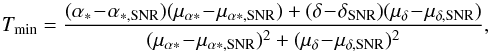 (5)which can be substituted back into Eq. (4) to obtain the minimum separation Δθmin.
We construct the covariance matrix Cov = D1/2CorrD1/2 using the correlation matrix Corr and the diagonal matrix of errors  which are given in TGAS. We have added on the 0.3mas systematic error in parallax recommended by Gaia Collaboration (2016a). We draw samples from the multivariate Gaussian distribution defined by the mean position (α,δ,ω,μα,μδ) and the covariance matrix Cov and from the distributions of the SNR centre, distance and peculiar velocity. These latter distributions are described in Sect. 2.2. We calculate Tmin and θmin for each of the samples which can be combined into distributions for the predicted minimum separation and time at which it occurs.
Once we have these distributions we classify stars by the plausibility of them being the former companion. We do this in a qualitative way by finding the fraction F of realizations of each star which satisfy 1 < (Tmin/ kyr) < 150, the line-of-sight distance between the star and the SNR is less than 153pc and has θmin corresponding to a physical separation less than 1pc. The latter two of these constraints use the distance to the location of the progenitor binary when the supernova exploded which can be calculated using the sampled parameters and the time of the minimum separation. The 153pc limit of the second constraint is simply the distance travelled by a star at 1000kms-1 over 150kyr and is the maximum likely distance travelled by a runaway associated with a SNR. The 1pc limit of the third constraint is approximately the maximum likely separation of two stars in a binary and is smaller than the 153pc limit in the radial direction because we have a measurement of the proper motion of each candidate. The value of F is shown for every star in each SNR in Fig. 1.
We rank the candidates in each SNR by this quasi-statistical measure and consider the star with the highest F to be the most likely candidate. For some of these stars, we can obtain APASS B−V photometry from a TGAS/APASS cross-match and, were this method effective, most of the best candidates would be blue. Of the ten best candidates two have no associated B−V in the cross-match and five have B−V> 1.3 hence are unlikely to be OB stars. One of the two best candidates without a measured B−V was HD 37424 in G180.0−01.7 (S147), which is one of the only five stars in G180.0−01.7 which did not have APASS magnitudes. HD 37424 has been previously suggested to be the runaway companion of G180.0−01.7 (Dinçel et al. 2015) and taking B−V = 0.073 ± 0.025 from that paper we see that our kinematic method would have proposed this star as a candidate if it had magnitudes in APASS. The remaining three stars with magnitudes are TYC 2688-1556-1 in G074.0−08.5 (Cygnus Loop) with B−V = 0.43, BD+50 3188 in G089.0+ 04.7 (HB 21) with B−V = 0.39 and TYC 4280-562-1 in G114.3+ 00.3 with B−V = 0.39. Of these stars only BD+50 3188 is specifically mentioned in the literature with Chojnowski et al. (2015) concluding that it is a B star. That one of the stars is B type suggests that the other two stars with similar colour are also B type by association, although it is possible that these two stars are less reddened by interstellar dust. G089.0+ 04.7 is at a distance of 1.7 ± 0.5kpc while the other SNRs are much closer at  and 0.70 ± 0.35kpc. The consequence of the B−V measurement being less reddened by dust is that the star is intrinsically redder and so the two untyped candidates may be A type or later.
This conclusion has some obvious problems. First, we have not established what fraction of runaways from core-collapse SNe we would expect to be later-type than OB. The distribution of mass ratios in massive binary systems is observed to be flat (e.g. Sana et al. 2012; Duchêne & Kraus 2013; Kobulnicky et al. 2014) which suggests that we would expect most runaways from core-collapse SNe to be bright, blue, OB-type stars. Thus, while it is possible to have low-mass companions of primaries with masses M> 8M⊙, around 80% of companions to massive stars will have masses in excess of 3M⊙ with a median of 7M⊙. This expectation is in conflict with the result above where five out of the ten best candidates are likely to be low-mass stars. One explanation for this seemingly large fraction of contaminants is that the method efficiently rules out those stars which are travelling in entirely the wrong direction to have originated in the centre of the SNR, but leaves in background stars which are co-incident on the sky with the centre of the SNR and whose proper motion is not constrained. This can explain the large fraction of our best candidates being stars whose photometry indicates that if they are at the distance of the SNR then they must be faint, red, late-type stars, because more distant stars will be more dust-obscured and so appear redder.
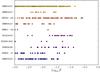 |
Fig. 1 The fraction F of realisations of each star in each SNR which are consistent with being spatially coincident with the centre of the SNR at one point in the past 150kyr. The criteria for determining whether a realisation is consistent are described in Sect. 3. |
A second problem is that, because we have not accounted for the reddening in E(B−V) in a quantitative way, the estimated spectral type of our candidates depended on one of them having already been typed. This estimated type is very uncertain, and two of the stars could be A type or even later. The method we used also did not make use of the Gaia G magnitude, despite it being the most accurate magnitude contained in the Gaia-APASS cross-match. Third, while we have generated a list of candidates, the ranking in the list is not on a firm statistical basis. There are four stars in G074.0−08.5 which have 0.25 <F< 0.28, only one of which is our best candidate. It is difficult to defend a candidate when a different statistical measure could prefer a different star. The fourth problem is that using the B−V photometry to further constrain our list of candidates relies on an expectation that most runaways from core-collapse supernova should be OB stars. Ideally our statistical measure should incorporate this prior but include the possibility that some runaways will be late-type.
These problems point towards the need for an algorithm that incorporates kinematics with photometry, dust maps and binary star simulations in a Bayesian framework.
4. Bayesian search with binaries, light and dust
4.1. Binary star evolution grid
The three most important parameters which determine the evolution of a binary star are the initial primary mass M1, initial secondary mass M2 and initial orbital period Porb. Empirical probability distributions have been determined for these parameters and combining these with a model for binary evolution allows us to calculate a probability distribution for the properties of runaway stars. The properties of runaway stars which we are interested in are the ejection velocity vej, the intrinsic colour (B−V)0 and the intrinsic Gaia G magnitude G0 at the time of the supernova.
There are two standard formalisms used when evolving a large number of binary stars to evaluate the probability distribution for an outcome. The first is Monte Carlo-based and involves sampling initial properties from the distributions and evolving each sampled binary. In this approach the initial properties of the evolved binaries are clustered in the high-probability regions of the initial parameter space and low-probability regions which may have interesting outcomes might not be sampled at all. The other method is grid-based and selects binaries to evolve on a regularly-spaced grid across the parameter space. This grid divides the parameter space into discrete elements (voxels) and the probability of a binary having initial properties which lie in that voxel can be found by integrating the probability distributions over the voxel. This probability is assigned to the outcome of the evolution of the binary that was picked in that voxel. The probability distribution for the runaway properties can be determined by either method. In the Monte Carlo approach the resulting runaways from the binary evolution are samples from the probability distribution for runaway properties while in the grid approach the distribution can be obtained by summing the probabilities which were attached to the runaway from each evolved binary.
Our choice of a grid over a Monte Carlo approach was motivated by our need to probe unusual areas of the parameter space. A Monte Carlo approach would require a large number of samples to fully explore these areas, while a grid approach gives us the location and associated probability of each voxel that produces a runaway star as well as the properties of the corresponding runaway star. These probabilities and other properties are thus functions of this initial grid.
We model the properties of stars ejected from binary systems in which one component goes supernova using the binary_c population-nucleosynthesis framework (Izzard et al. 2004, 2006, 2009). This code is based on the binary-star evolution (bse) algorithm of Hurley et al. (2002) expanded to incorporate nucleosynthesis, wind-Roche-lobe-overflow (Abate et al. 2013, 2015), stellar rotation (de Mink et al. 2013), accurate stellar lifetimes of massive stars (Schneider et al. 2014), dynamical effects from asymmetric supernovae (Tauris & Takens 1998), an improved algorithm describing the rate of Roche-lobe overflow (Claeys et al. 2014), and core-collapse supernovae (Zapartas et al. 2017). In particular, we take our black hole remnant masses from Spera et al. (2015) and use a fit to the simulations of Liu et al. (2015) to determine the impulse imparted by the supernova ejecta on the companion, both of which were options previously implemented in binary_c. We use version 2.0pre22, SVN 4585. Grids of stars are modelled using the binary_grid2 module to explore the single-star parameter space as a function of stellar mass M, and the binary-star parameter space in primary mass M1, secondary mass M2 and orbital period Porb.
We pre-compute this binary grid of 8 000 000 binaries with primary mass M1, mass ratio q = M2/M1 and orbital period Porb having the ranges, 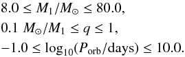 (6)We assume the primary mass has the Kroupa (2001) IMF,
 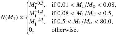 (7)We assume a flat mass-ratio distribution for each system over the range 0.1M⊙/M1<q< 1. We use a hybrid period distribution (Izzard et al. 2017) which gives the period distribution as a function of primary mass and bridges the log-normal distribution for low-mass stars (Duquennoy & Mayor 1991) and a power law (Sana et al. 2012) distribution for OB-type stars. The grid was set at solar metallicity to model recent runaway stars from nearby SNRs.
It is useful to distinguish between the runaway parameter space (B−V)0–G0–vej, which is best for highlighting the different runaway production channels, and the progenitor space M1–q–Porb, which is best for investigating the connection of those channels to other binary phenomena. For instance, our plot of runaway space in Fig. 2 has several gaps towards the top right, which, when viewed instead in the progenitor space, turn out to be regions where the binary has merged prior to the primary going supernova. There are several prominent trends in Fig. 2 which will be discussed in detail in a forthcoming paper. We note that most of the probability is concentrated on the left edge of the plot in slow runaways of all colours. These correspond to the scenario of binary ejection where the two stars do not interact and the ejection velocity is purely the orbital velocity of the companion at the time of the supernova. The rest of the structure corresponds to cases when at some point in the evolution the primary overflows onto the secondary and forms a common envelope (Izzard et al. 2012; Ivanova et al. 2013). The drag force of the gas on the two stellar cores causes an in-spiral, while the lost orbital energy heats and ejects the common envelope. These runaways are faster due to the larger orbital velocity from the closer orbit, but there is a small additional kick from the impact of SN ejecta on their surface.
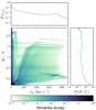 |
Fig. 2 Probability distribution in velocity-colour space of the runaways produced by our binary evolution grid. The top and right plots show 1D projections of the joint probability distribution. |
4.2. Algorithm
We want to assess the hypothesis that a given observed star with observables x is a runaway from a SNR. Our null hypothesis H0 is that a particular star is not the runaway companion and we wish to test this against the hypothesis H1 that it is. In Bayesian inference each hypothesis H has a set of model parameters θ which can take values in the region Ω. H is defined by a prior  and a likelihood ℒ(x | θ,H). The Bayesian evidence for the hypothesis is then
  , which is given by the integral
 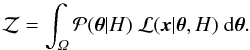 (8)The evidence is equivalent to Pr(x | H), i.e. the probability of the data given the hypothesis.
To compare the background (H0) and runaway (H1) hypotheses we calculate the Bayes factor  , where
  and
and  are the evidences for H0 and H1 respectively. The interpretation of Bayes factors is subjective but a Bayes factor greater than one indicates that H1 is more strongly supported by the data than H0 and vice versa. A review on the use of Bayes factors is given by Kass & Raftery (1995) who provide a table of approximate descriptions for the weight of evidence in favour of H1 indicated by a Bayes factor K. To aid the interpretation of our results we replicate this table in Table 2.
Subjective interpretation of Bayes factors K (taken from Kass & Raftery 1995).
To obtain the evidence for H0 we define a probability distribution using the stars in the TGAS/APASS cross-match that lie in an annulus of width 10° outside the circle from which we draw our candidates. Assuming that the locations of the stars in the space (ω,μα ∗,μδ,G,B−V) can be described by a probability distribution we can approximate that distribution in a non-parametric way by placing Gaussians at the location of each star and summing up their contributions over the entire space. This method is called kernel density estimation (KDE). Note that we normalise the value in each dimension by the standard deviation in that dimension for the entire sample. This normalisation is necessary because the different dimensions have different units. The prior for each candidate is a Gaussian in each dimension centred on the measured value with a standard deviation given by the measurement error. The likelihood for a point sampled from the prior is the KDE evaluated at that point. Strictly speaking this is the wrong way round. The KDE should define the prior and the likelihood should be a series of Gaussians centred on the data, but, since the definition of the evidence is symmetric in the prior and likelihood (Eq. (8)), we are free to switch them.
The evidence for H1 is more complicated to calculate because the model parameters θ are properties of the SNR and progenitor binary and thus need to be transformed into predicted observables  of the runaway. The likelihood is
  (9)where is a function of θ and
  denotes the PDF of a multivariate Gaussian distribution evaluated at a with mean b and covariance matrix C. For this preliminary work we neglect the off-diagonal terms of the covariance matrix.
Model parameters for the runaway hypothesis.
The prior combines the primary mass M1, mass ratio q and period Porb of the progenitor binary with the location (αSNR, δSNR), age tSNR, distance dSNR and peculiar velocity vpec of the SNR and the reddening E(B−V) along the line of sight. These model parameters are given in Table 3 for reference. The prior is 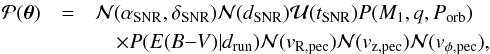 (10)where
  denotes a univariate Gaussian distribution in a,
  denotes a multivariate Gaussian distribution in a and b,
  denotes a uniform distribution in a and the other components are non-analytic. The additional variable drun is the predicted distance between the observer and runaway and is a function of the other model parameters. The ranges, means and standard deviations for the first three and last three distributions are given in Sect. 2.2 and were used for the simple method in Sect. 3.
The function P(M1,q,Porb) is the probability that, if there is a runaway star, it originates in a progenitor binary with those properties. This probability can be obtained directly from the PDFs of the binary properties (Sect. 4.1) after renormalising to remove the binaries which do not produce runaway stars.
The other non-analytic function P(E(B−V) | drun) expresses the probability of the reddening along the line of sight to the observed star if it is at a distance drun. Green et al. (2015) used Pan-STARRS 1 and 2MASS photometry to produce a 3D dustmap covering three quarters of the sky and extending out to several kiloparsec. Green et al. (2015) provide samples from their posterior for E(B−V) in each distance modulus bin for each HEALPix (nside= 512, corresponding to a resolution of approximately 7arcmin) on the sky. We use a Gaussian KDE to obtain a smooth probability distribution for E(B−V) in each distance modulus bin. We then interpolate between those distributions to obtain a smooth estimate of P(E(B−V) | μ) which we illustrate for one sight-line towards the centre of S147 in Fig. 3. Note that log 10drun = 1 + μ/ 5, where drun is a function of our other model parameters. Green et al. (2015) used the same definition of E(B−V) as Schlegel et al. (1998) so we have converted their E(B−V) to the Landolt filter system using coefficients from Schlafly & Finkbeiner (2011).
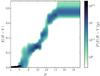 |
Fig. 3 The conditional PDF for the dust extinction along the line of sight to G180.0−1.7 calculated by interpolating samples from the Green et al. (2015) dust map. |
The rest of this section is devoted to describing the transform  between the model parameters and the predicted observables. The outcome of the binary evolution is a function solely of the progenitor binary model parameters. The pre-calculated grid of binary stars thus provides the ejection velocity vej, intrinsic colour (B−V)0 and intrinsic magnitude G0, which are essential to mapping the model parameters to predicted observables. In addition, we obtain other parameters of interest such as the present day mass of the runaway star Mrun and the age Trun.
The kinematics of the SNR centre are fully determined by the position, distance and peculiar velocity, under the assumption that the velocity is composed of a peculiar velocity on top of the rotation of the Galactic disk at the location of the SNR centre. The location of the runaway on the sky is known because the errors on the observed position of a star with Gaia are small enough to be negligible. The remaining kinematics that need to be predicted are the distance drun and proper motion. The velocity vector of the runaway vrun is the sum of the velocity of the SNR and the ejection velocity vector vej. The location of the explosion, now the centre of the SNR, continues along the orbit of the progenitor binary within the Galaxy. We advance the centre of the SNR and the runaway along their orbits for the current age of the SNR tSNR, noting that this time is so short that any acceleration is negligible and thus the orbits are essentially straight lines. The separation of the centre of the SNR and the runaway at this point is then simply the difference of their velocity vectors multiplied by tSNR, i.e. vejtSNR. We then fix the kinematics of the model by denoting the present-day centre of the SNR to be at (αSNR,δSNR) and the present-day distance to the centre of the SNR to be dSNR.
To obtain predictions for the proper motions and parallax we consider the intersection of the half-line defined by the observed position of the candidate on the sky and a sphere centred at the distance and position of the SNR. This sphere has a radius given by vejtSNR, which is the distance travelled by the runaway since the supernova. A diagram of this geometry is shown in Fig. 4. If the distance travelled by the runaway is not large enough then the sphere fails to intersect the line and thus the likelihood of this set of parameters is zero. In almost every case there are two intersections which correspond to the runaway moving either away from or towards us. If the SNR is close and old and the runaway is travelling rapidly, there is a pathological case in which there is only one solution because the solution which corresponds to a runaway moving towards us is already behind us. The geometry of the intersection point gives us the distance to the star which we can use to predict the parallax. The predicted proper motion of the runaway depends on the velocity of progenitor binary. We sample in the velocity dispersion of the Milky Way thin disk and add on the rotation of the disk and ejection velocity of the runaway. This velocity is converted to proper-motions and line-of-sight radial velocities using the transforms of Johnson & Soderblom (1987).
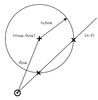 |
Fig. 4 A diagram of the geometry described in Sect. 4.2. The observer is at ⊙ and the centre of the supernova remnant is at +. The two possible locations of the candidate if it is the runaway are marked by × and correspond to the intersection of the sphere of radius vejtSNR centred on the SNR and the half-line defined by the coordinates of the candidate. |
We then obtain a prediction for B−V by simply using B−V = (B−V)0 + E(B−V). The Gaia G band is broader than the V band and so is more sensitive to the slope of the spectrum (Sanders et al., in prep.). One consequence of this is that the relative reddening in the G band A(G) /A(V) is a function of the intrinsic colour of the star. Assuming that A(V) = RVE(B−V), where the constant RV = 3.1 is related to the average size of the dust grains and has been empirically determined in the Milky Way (Schultz & Wiemer 1975), we recast this dependency as A(G) /E(B−V) as a function of (B−V)0. This relation has been calculated empirically by Sanders et al. (in prep.) and thus we have an expression for the apparent magnitude G = G0 + A(G) + μ.
We elected to use nested sampling (Skilling 2006) to explore the parameter space since it is optimised with estimating the evidence as the primary goal while more standard Markov Chain Monte Carlo (MCMC) methods are targeted at obtaining samples from the posterior which afterwards can be used to estimate the evidence. We use the MultiNest implementation of nested sampling (Feroz & Hobson 2008; Feroz et al. 2009, 2013) which we access through the PyMultiNest Python module (Buchner et al. 2014). MultiNest requires that we express our prior as a transform from a unit hypercube to the space covered by our prior. For independent parameters, this is a trivial application of inverting the cumulative distribution function. However, we have two prior probability distributions P(E(B−V) | μ) and P(M1,q,Porb) for which there are no suitable transforms. Note that μ is the distance modulus to the runaway which is a complicated function of the position, distance and age of the SNR and the ejection velocity of the runaway. For these parameters, we use the standard method of moving the probability distribution into the likelihood, which is implemented in MultiNest by assuming a uniform distribution in the prior and including a factor in the likelihood to remove this extra normalisation. Some technical details of the implementation of MultiNest are discussed in Appendix B.
Using nested sampling, we explore the parameter space and obtain a value for the log of the evidence for each candidate. We then obtain the Bayes factor by dividing the evidence for H1 by the evidence for H0. A Bayes factor less than one indicates that the null hypothesis is more strongly favoured, i.e. this star is likely a background star. A Bayes factor greater than one suggests that the runaway model is preferred.
4.3. Fraction of supernovae with runaways
Only a fraction of supernovae will result in a runaway companion. Some massive stars are born single and companions are not always gravitationally unbound from the compact remnant after the supernova. Companions of massive stars tend to also be massive and so some will themselves explode as a core-collapse supernova, either in a bound system with the compact remnant of the primary or after being ejected as a runaway star (e.g. Zapartas et al. 2017). A further contaminant is that binary evolution can cause stars to merge before the primary supernova occurs, through dynamical mass transfer leading to a spiral-in during common envelope evolution. Our model assumes that there was a runaway companion to the SNR and thus the calculated evidence needs to be multiplied by the fraction of SNRs with a runaway.
Evolving a population of binary stars as described above we find that the average number of core-collapse supernovae per binary system with a primary more massive than 8M⊙ is 1.22. All single stars in the mass range 8 <M/M⊙< 40 are expected to go supernova, with most stars more massive than 40M⊙ probably collapsing directly to black holes (Heger et al. 2003). Note that in the version of binary_c used for this work a core-collapse supernova is signalled whenever the core of a star collapses to a neutron star or black hole, including the case where the primary collapses directly to a black hole. Such collapses are sufficiently rare that we do not correct for this effect. An assumption on the binary fraction is required to combine statistics for single and binary populations. Arenou (2010) provides an analytic empirical fit to the observed binary fraction of various stellar masses,  (11)Based on this binary fraction and grids of single and binary stars evolved with binary_c we estimate that 32.5% of core-collapse supernovae have a runaway companion. This fraction is best described as “about a third” given the approximate nature of the prescriptions used to model the binary evolution and the uncertainties in the empirical distributions of binary properties.
4.4. Verification
We verify our calculation of the evidence above by sampling runaways from the model and using their (ω, μα, ∗, μδ, G,B−V) to generate a kernel density estimate of their PDF. The evidence for a candidate to be a runaway can then be computed identically to the background evidence. In contrast to the method described in Sect. 4.2, where the prior and likelihood are functions of the model parameters which are described in Table 3, this method casts the prior and likelihood as a function of the model observables. In the limit where we draw infinite samples from our model this method will give the same result as the method in Sect. 4.2. Drawing samples from the model and constructing a KDE is advantageous for its simplicity. The likelihood function is an evaluation of a KDE and thus is guaranteed to be smooth and non-zero everywhere, meaning that the considerations discussed in Appendix B are not relevant. The first disadvantage of calculating the evidence by this method is that it only gives accurate values of the evidence for regions of the parameter space which are well sampled. The second disadvantage is that by not being explicit about the model parameters we cannot directly constrain them, and so this method does not output the maximum-likelihood distance to the SNR or the mass of the progenitor primary. The implicit method is used in this work solely as a cross-check of our results.
4.5. Validation
We validate our method by considering approximations to the false positive and the false negative rate. For each SNR we assume there is a nominal SNR at Galactic coordinates (l,b) = (lSNR−1°,bSNR) with the same distance and diameter estimates as the true SNR. We acquire candidates from our TGAS and APASS cross-match and inject an equal number of model runaway stars sampled from our binary grid, calculating equatorial coordinates, parallaxes and proper motions which would correspond to a runaway from that location ejected in a random direction. These artificial measurements are convolved with a typical covariance matrix of errors, here using the mean covariance matrix in our list of candidates for this nominal SNR. For the dust correction, we randomly select one of the twenty samples provided by the Green et al. (2015) dustmap in each distance modulus bin along each line of sight, corresponding to the sight-line and distance modulus that we have sampled for the runaway. The injected runaways and real candidates are shuffled together so that the algorithm described in Sect. 4.2 is applied in the same manner to both the real stars and fake runaways. Since there is not a real SNR at this location all the real stars selected from the cross-match should be preferred to be background stars, while by construction the fake injected runaways should prefer the runaway hypothesis. An injected runaway which returns a Bayes factor K< 1 is a false negative and a real star with K> 1 is a false positive.
At the bottom of Fig. 5, we show the calculated Bayes factor K for all the real stars and injected stars. There are 217 stars in each series. Only three of the real stars are returned as false positives giving a false positive rate of 1.3%. All three of these false positives are from the fake version of G065.3+ 05.7 which we find is because of the large photometric errors of APASS in this field. These errors are around ± 0.142 in B−V which compare to ± 0.055mag for G180.0−01.7. This suggests that the millimag precision of the GBP and GRP bands in Gaia DR2 will further reduce the false positive rate.
There are 22 false negatives which corresponds to a false negative rate of about 10%. Given that we only expect a third of SNRs to have an associated runaway companion (see Sect. 4.3) and that we only consider ten SNRs, we should have at most one false negative in our observed sample.
We note that there are more stars closer to the 2lnK = 0 boundary in our science runs (above the line in Fig. 5) than were found in the false positive test. This is because runaways are more likely to be OB stars and that OB stars are typically found in star-forming regions. If a SN has occurred then a star-forming region is nearby and so there are OB stars in or close to the SNR which act as contaminants.
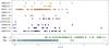 |
Fig. 5 Bayes factors for the hypothesis that each star in each SNR is a runaway star versus the hypothesis that it is a contaminant. The false positive and false negative series are described in Sect. 4.5. |
5. Results
We report the seven stars for which the Bayes factor is greater than one by at least the error on the evidence estimated by MultiNest. In Fig. 5, we show the calculated Bayes factor K for the candidates in each SNR over the range (− 20,20). In Sect. 5.1 we discuss the three contaminant stars which we are able to rule out and in Sect. 5.2 we analyze each of the four real candidates individually. Three of our candidates are new while HD 37424 in S147 has previously been suggested by Dinçel et al. (2015).
The only SNR in common with the search for OB runaways by Guseinov et al. (2005) is G089.0+ 04.7 and they proposed a different candidate, GSC 03582−00029. This star appears to be significantly brighter in the infrared (J = 10.2,H = 9.7,K = 9.6) than in the optical (B = 11.9) while an OB star should have B−K = −1 (Castelli & Kurucz 2004), so the classification of this star as OB seems unlikely.
Table of median posterior values for our new candidates.
5.1. Eliminating the contaminants
In Fig. 5, there are seven stars which have Bayes factors greater than one. The presence of two of these stars for G074.0−08.5 makes it clear that there is at least some level of contamination. We found empirically that there are two ways to produce false positives in our model. First, if the star is a high proper-motion star in the foreground then the evidence for it in the background model can be spuriously low. This can occur because the background is constructed by taking a kernel density estimate of stars around the SNR and it may not contain enough foreground stars to reproduce this population. A low evidence in favour of the background model boosts the Bayes factor so that the runaway model is preferred, even if the star would be a very low-likelihood runaway. Second, if the errors on the photometry from APASS are greater than around 0.1mag in each of B and V then it is possible for the algorithm to ascribe a high probability to a far-away blue star when the candidate is actually a nearby red star. This increases the likelihood in favour of the runaway hypothesis.
If a contaminant is caused by the first of these possibilities, then this is clear from an unusually jagged posterior of the runaway model. Foreground high proper-motion stars tend to not be OB stars and so to explain the star under the runaway hypothesis MultiNest is forced to sample in regions of the progenitor binary parameter space that produce fast, red runaways. These are rare and lie in the region to the top right of Fig. 2 that is not well sampled in the binary grid because there are very few of them. This under-sampling results in a jagged posterior dominated by spikes of high probability, with reported modes that are poorly converged with large errors on  . The stars with the highest Bayes factor in both G074.0−08.5 and G160.9+ 02.6 are contaminants of this first kind, which can clearly be seen in Fig. 5 as both these stars have much broader error bars than the typical candidate.
The second type of contaminant is only a problem in this work because we have chosen to take the photometry from APASS for all the SNRs, while for some fields Tycho2 has much smaller errors. This is mainly caused by a known problem in measurements taken for APASS DR8 in northern fields where the blue magnitudes have larger errors than expected2. If the best measurement of B−V has a large error then the problem discussed above is a feature, because the Bayesian evidence is the likelihood integrated against the probability of every possible combination of model parameters. The star with the highest Bayes factor in G065.3+ 05.7 is one such contaminant. BD+30 3621 was the only star in G065.3+ 05.7 with a Bayes factor greater than one. APASS reports a measurement (B−V) = 1.10 ± 0.88 for this star, but MultiNest picked out a most likely value of (B−V)0 = −0.22 ± 0.02. The Tycho 2 catalogue reports B−V = 1.37 ± 0.02 confirming BD+30 3621 as a late-type star. The large measurement error reported in APASS allowed the model to explore parameter space where this star is much bluer than in reality. This is a preliminary study in preparation for Gaia DR2, which will provide GBP and GRP with millimag precision across the entire sky. This second type of contaminant will not be a problem in Gaia DR2, because there will not be more accurate photometry that we could use to ‘double check’ the measurements.
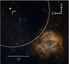 |
Fig. 6 Digitized Sky Survey image of the vicinity of the Rosette Nebula. The runaway star candidate HD 261393 is marked by a white cross, the white cross hairs indicate the geometric centre of the Monoceros Loop and the white circle approximately shows the inner edge of the Monoceros Loop shell. The Rosette Nebula is in the bottom right and the Mon OB2 association extends 3° to the east and north-east towards the centre of the Monoceros Loop. |
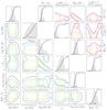 |
Fig. 7 Corner plots of the posterior samples from the model of TYC 2688-1556-1 in G074.0−08.5 with 1σ, 2σ and 3σ contours. The 1D histograms include the CDF of that parameter and the error bars indicate the median and 1σ errorbars of each mode. Bottom left: a corner plot showing the model parameters, excluding the five parameters related to the position and peculiar velocity of the SNR which did not have covariances with the other parameters. Top right: a corner plot showing a selection of the derived parameters which are functions of the model parameters. |
5.2. Individual candidates
TYC 2688-1556-1 The star TYC 2688-1556-1 in G074.0−08.5 (Cygnus Loop) has no known references in the literature. It is a relatively high proper-motion star with (μα ∗,μδ) = (3.92 ± 0.83,−21.03 ± 1.25)masyr-1 reported in TGAS. The colour and magnitude of this star in the TGAS/APASS cross-match suggest this star is likely A type, which agrees with the posterior for the current mass of the runaway of 1.73 ± 0.13M⊙. The posterior for the ejection velocity includes a second mode which corresponds to the clump of stars at vej = 700kms-1 in Fig. 2. Runaways in this region of (B−V)0−vej space have undergone significant mass exchange with the primary and will have had a common envelope phase. This mass exchange shrinks the orbit of the binary which increases the orbital velocity and is the origin of the high velocity of these stars. If this mode is the true origin of TYC 2688-1556-1, then the star is predicted to have lost several solar masses of material, having started off at around 6M⊙ and ended with around 2M⊙. In this case the star may be chemically peculiar. A more prominent observable of this channel is that it would predict a heliocentric radial velocity around + 600kms-1 or −600kms-1, where the uncertainty is due to the degeneracy in whether the star is moving towards or away from us. Looking at Fig. 7, this degeneracy appears as a “v”-shaped contour in the vr–vej plot. If the star is from this mode, it is likely unbound from the Milky Way. The covariance in the most probable mode between M1 and q is simply the relationship M2 = qM1 = const. This covariance is interpreted as there being minimal mass transfer in the binary system so that the mass of the runaway now is approximately the mass it was born with. The secondary mode is clearly visible as lying off this relationship.
BD+50 3188 The B-type star BD+50 3188 in G089.0+ 04.7 exhibits emission lines in its spectra and so is classed as a Be star (most recently studied by Chojnowski et al. 2015). The emission lines in Be stars are thought to originate from a low-latitude disk or ring-like envelope (Kogure & Leung 2007), which in the case of BD+50 3188 is measured to be rotating at 138kms-1 (Chojnowski et al. 2015). Be stars are also characterised by rapid rotation, which can be close to their break-up speed, and this is thought to be related to their formation mechanism (Kogure & Leung 2007). Be stars are observed in both single and binary systems. There are plausible formation mechanisms in the literature which can produce Be stars that are single or binary (Kogure & Leung 2007). A Be star can be formed if it is the mass gaining component in a binary in the Roche-lobe Overflow (RLOF) phase (see Harmanec 1987) where the emission-lines originate in the accretion disk formed of material lost by the Roche-lobe filling companion. Pols et al. (1991) argues that the duration of the RLOF phase, and hence the lifetime of the accretion disk, is not sufficiently long to explain the high fraction of B type stars which are Be stars. Pols et al. (1991) instead propose the post-mass-transfer model where most Be stars are in systems after the end of RLOF. During RLOF the mass-gaining component is spun up by the angular momentum of the accreted mass. If the mass gainer is rotating at close to break-up by the end of the RLOF phase we may see emission-lines from a decretion disk around the equator of the star. Shortly after the RLOF phase, the mass loser in such a system detonates as a supernova which may unbind the system and produce a runaway Be star (Kogure & Leung 2007). Rinehart (2000) used proper-motions from Hipparcos to compare the velocity distributions of B and Be type stars and, finding that they were consistent to within 1σ, argued that they were not consistent with most Be type stars being runaways. Berger & Gies (2001) performed a similar analysis but with the inclusion of radial velocities and found instead that around 7% of Be stars have large peculiar velocities. Berger & Gies (2001) points out that the runaway fraction among all B stars is about 2% and thus this result alone supports a runaway origin for at least some Be stars. Berger & Gies (2001) goes on to argue that the fraction of Be stars which have been spun up by binary interaction is unknown, because some binaries will remain bound post-supernova (Be + neutron star binary) and others will either be low-mass or experience extreme mass-loss and bypass the supernova altogether (Be + Helium star or Be + white dwarf binaries). In more recent work, de Mink et al. (2013) modelled massive binary stars and found that it is possible for all early-type Be stars to originate in binaries through mass transfer and mergers. Rivinius et al. (2013) review the origin and physics of Be stars and conclude that the emission-lines in a majority of the systems are due to a decretion disk around a rapidly rotating star, however they conclude that binarity is not a widespread mechanism because the statistical properties of B and Be binaries appear to be identical (Abt & Levy 1978; Oudmaijer & Parr 2010). BD+50 3188 is the only Be star within a 2° radius of G089.0+ 04.7 and is only 2.4arcmin from the centre. That it is a Be star with no known binary companion which is spatially co-located with the SNR lends circumstantial evidence to it being the runaway companion of G089.0+ 04.7.
HD 37424 This star is our most likely candidate with a Bayes factor K of 2lnK = 17.72 ± 0.13. A connection between this star and the SNR G180.0−01.7 was previously drawn by Dinçel et al. (2015) who used the kinematics of the star and the associated central compact object PSR J0538+2817 to show both were in the same location 30 ± 4kyr ago. Dinçel et al. (2015) estimated that this star has spectral type B0.5V ± 0.5 and a mass around 13M⊙, while our method found Mrun = 10.38 ± 1.04M⊙. Dinçel et al. (2015) used this mass and the lack of nearby O-type stars to argue that the progenitor primary must have a mass that is at most 20–25M⊙, with the possibility that the system may have been a twin binary. The most likely mode in our posterior (Fig. 9) corresponds to a scenario where the initial masses in the binary were M1 = 20 ± 5M⊙ and M2 = 7 ± 2M⊙. Our favoured initial primary mass is consistent with the lack of O-type stars while we find that the secondary has actually increased in mass because of mass transfer from the primary to the companion. The possibility of a twin progenitor binary is strongly excluded under our model.
Similarly to Sect. 3 we took B−V = 0.073 ± 0.025 from Dinçel et al. (2015) because HD 37424 is one of the five stars in G180.0−01.7 without APASS photometry. We were motivated to investigate this star despite it not having APASS photometry because it had been previously suggested to be the runaway companion.
HD 261393 The star HD 261393 in G205.5+ 00.5 is given a spectral type of B5V by Voroshilov et al. (1985) who also assigned it membership of NGC 2244, an open cluster at the centre of the Rosette Nebula. However, HD 261393 is  from the centre of the Rosette Nebula (Fig. 6), so it is more likely to be a member of the adjoining Monoceros OB2 association which extends to the east and north-east by several degrees. Odegard (1986) established that the Monoceros Loop is within the Mon OB2 association and is interacting with, and lies behind, the Rosette Nebula. This conclusion was supported by later work (see Xiao & Zhu 2012, for a review). Martins et al. (2012) modelled the stellar properties of ten O type stars in NGC 2244 and the surrounding Monoceros OB2 association and found that the age of the stars is in the range 1–5Myr. In order for HD 261393 to be a runaway with an age less than 5Myr, our model would require the primary of the progenitor binary to be at least 40M⊙. In the posterior shown in Fig. 10 a primary of this mass would lie between the 2 and 3σ contours. This extra constraint would decrease the Bayesian evidence for a runaway origin and may be enough to result in the background being more favourable. A similar line of reasoning for the mass of the primary was put forward by Gebel & Shore (1972) who argued that the minimum possible mass of the progenitor must exceed the 25M⊙ mass of the most massive O star in the SNR. The models used by Martins et al. (2012) to estimate the age of Mon OB2 did not include the possibility of rejuvenation by mass transfer or merger in binaries which can result in an underestimated age of OB associations (e.g. Schneider et al. 2014 used binary evolution simulations to predict that the 9 ± 3 and 8 ± 3 most massive stars in the Arches and Quintuplet star clusters respectively are likely merger products). Including the possibility of binary evolution would increase the estimated age of the Mon OB2 association and thus decrease the tension with our model. Gebel & Shore (1972) further speculated that the B type star HD 258982 might be the associated runaway star because it is the only B type star observed at that time in the SNR which displays the CaK absorption line at the 16kms-1 of the expanding SNR shell. HD 258982 is around
  away from the geometric centre of the Monoceros Loop and the proper motion of this star had not been measured at the time of Gebel & Shore (1972). In TGAS, this star has a measured proper motion of around 3masyr-1 meaning that the star can have travelled at most
  in the 150kyr age of the SNR and is effectively ruled out as a possible candidate.
6. Conclusions
We have used two methods to search for and quantify the significance of runaway former companions of the progenitors of nearby SNRs. The first method used kinematics from the Tycho-Gaia astrometric solution (TGAS) to find the star most likely to have been spatially coincident with the SNR centre in the past 150kyr and further filtered those candidates based on their B−V colour. This filtering was done to select likely OB stars. The second method is more elaborate and was designed to make full use of the available photometry, to incorporate 3D dustmaps, to be explicit about our expectation that most but not all runaways are OB type, and to be statistically rigorous. This Bayesian method has the advantage that it constrains the properties of both the progenitor binary and the present day runaway.
Both methods returned four candidates and reassuringly three of those were in common. These are TYC 2688-1556-1 in G074.0−08.5, BD+50 3188 in G089.0+ 04.7 and HD 37424 in G180.0−01.7. The remaining candidate from the kinematic method is TYC 4280-562-1 in G114.3+ 00.3 which has 2lnK = −4.69 ± 0.14 in the Bayesian method and thus is the seventh most likely runaway in this SNR. The remaining candidate from the Bayesian method is HD 261393 in G205.5+ 00.5, which was ranked fourth in this SNR by the kinematic method.
Three of the candidates proposed by our Bayesian method are new, while HD 37424 was previously suggested by Dinçel et al. (2015). It is reassuring that this star was picked out by both methods and was already in the literature. It has a Bayes factor K of 2lnK = 17.72 ± 0.13, which makes it a very strong candidate. The posterior suggests that this star may have gained several solar masses from the primary prior to the supernova. The best of our new candidates is BD+50 3188. This is a Be star which can be explained by the star being spun up by mass transfer from the primary prior to the supernova. It is also the only Be star within several degrees of this SNR and is only 2.4arcmin from the geometric centre. If TYC 2688-1556-1 is the runaway companion of G074.0−08.5 then it is likely to be an A type. There is a second mode in the posterior for TYC 2688-1556-1 which would correspond to this star having mass transferred onto its primary. It predicts that this star may be chemically peculiar and have a velocity greater than 600kms-1, making it a hypervelocity star. The final candidate from the Bayesian method is HD 261393. It is possible that the progenitor of the Monoceros Loop is part of the recent burst of star formation that has occurred in the Mon OB2 association over the last 1–5Myr. If this is true, then this extra constraint may mean HD 261393 is more likely to be a background star.
The method that Dinçel et al. (2015) used to propose HD 37424 as a candidate was based on a coincident spatial location with the pulsar in the past and thus is independent from our method which relates the star to the properties of the SNR. One advantage of our method is that it does not require there to be a known associated pulsar. Our Bayesian method could be altered to include stellar radial velocities and pulsar properties. The radial velocities would be an additional constraint on the model, the pulsar parallax could provide a more accurate distance to the SNR, and the pulsar proper motion combined with a time since the SN would set the location of the progenitor binary at the time of the SN. Gaia is aiming to provide radial velocities for a bright subset of the main photometric and astrometric sample. It is estimated that for a B1V star with apparent magnitude V = 11.3 the end-of-survey error on the radial velocity3 will be 15kms-1 which is sufficiently precise for tight constraints to be placed on runaway candidates.
A requirement of our Bayesian framework is the probability of a SNR to have a runaway companion. Accounting for single stars, merging stars, binaries that remain bound post-supernova and runaways that themselves go supernova, we find that one third of core-collapse SNRs should have a runaway companion. In agreement with this result, we find three runaway candidates from the ten SNRs considered.
As mentioned previously, Kochanek (2017) ruled out runaway companions of the Crab, Cas A and SN 1987A SNRs with initial mass ratios q ≳ 0.1. Including this null result for these three SNRs does not change our conclusion that the number of runaway candidates is consistent with the expected number of runaways, but if our two weaker candidates (TYC 2688-1556-1 and HD 261393) are subsequently ruled out a significant tension could arise. The SNRs considered by Kochanek (2017) are all younger (tSNR< 1kyr) and more distant (dSNR> 2kpc) than our SNR sample, making the two works complementary. The advantage of considering young SNRs is that a runaway companion is constrained to be much nearer to the centre of the SNR which limits the region that must be searched. The main disadvantage is the lack of parallaxes for distant stars which makes it harder to exclude candidates because of the degeneracy between distance, reddening and photometry. In terms of method Kochanek (2017) used PARSEC isochrones to carry out a pseudo-Bayesian fit to the photometry of each star while accounting for the distance and extinction to the SNR, which we would categorize as a middle ground between our simple and fully Bayesian approaches. Kochanek (2017) noted that a full simulation of binary evolution was beyond the scope of their work. It is the integration of binary evolution with a fully Bayesian method which is the main advance of this work. Future Gaia data releases will allow our fully Bayesian method to be applied to both the Crab and Cas A SNRs.
Gaia Data Release 2 (DR2) will contain positions, parallaxes, proper-motions and G, GBP and GRP for over a billion stars. This dataset is the reason for constructing our Bayesian framework. The millimagnitude precision of the photometry will remove poorly measured stars as contaminants, while the milliarcsecond precision of the parallaxes will remove high proper-motion foreground stars. The final Gaia data release aims to be complete down to G ≈ 20.5 and at that completeness we will be able to test the existence of a runaway companion for all the nearby SNRs.
Future spectroscopic observations of BD+50 3188, TYC 2688-1556-1 and HD 261393 will test whether they truly are SN companions, allowing them to be used to test binary star evolution. With Gaia DR2 in early 2018, our Bayesian framework provides a sharp set of tools that will allow us to find any runaways there are to find.
Green (2014), “A Catalogue of Galactic Supernova Remnants (2014 May version)”, Cavendish Laboratory, Cambridge, United Kingdom (available at http://www.mrao.cam.ac.uk/surveys/snrs/).
Green (2014), “A Catalogue of Galactic Supernova Remnants (2014 May version)”, Cavendish Laboratory, Cambridge, United Kingdom (available at http://www.mrao.cam.ac.uk/surveys/snrs/).
Acknowledgments
We thank Sergey Koposov, Vasily Belokurov, Jason Sanders and other members of the Streams group at the Institute of Astronomy in Cambridge for comments while this work was in progress. We also thank Gerry Gilmore for early discussions on this work. We are especially appreciative of Mathieu Renzo, Simon Stevenson, Manos Zapartas and the many other authors cited above who have contributed to the development of binary_c. DPB is grateful to the Science and Technology Facilities Council (STFC) for providing Ph.D. funding. M.F. is supported by a Royal Society – Science Foundation Ireland University Research Fellowship. This work was partly supported by the European Union FP7 programme through ERC grant number 320360. RGI thanks the STFC for funding his Rutherford fellowship under grant ST/L003910/1 and Churchill College, Cambridge for his fellowship. This work has made use of data from the European Space Agency (ESA) mission Gaia (https://www.cosmos.esa.int/gaia), processed by the Gaia Data Processing and Analysis Consortium (DPAC, https://www.cosmos.esa.int/web/gaia/dpac/consortium). Funding for the DPAC has been provided by national institutions, in particular the institutions participating in the Gaia Multilateral Agreement. This research has made use of the APASS database, located at the AAVSO web site. Funding for APASS has been provided by the Robert Martin Ayers Sciences Fund. Figures 2 and 3 made use of the cubehelix colour scheme (Green 2011).
References
- Abate, C., Pols, O. R., Izzard, R. G., Mohamed, S. S., & de Mink, S. E. 2013, A&A, 552, A26 [NASA ADS] [CrossRef] [EDP Sciences] [Google Scholar]
- Abate, C., Pols, O. R., Stancliffe, R. J., et al. 2015, A&A, 581, A62 [NASA ADS] [CrossRef] [EDP Sciences] [Google Scholar]
- Abt, H. A., & Levy, S. G. 1978, ApJ, 36, 241 [Google Scholar]
- Altmann, M., Roeser, S., Demleitner, M., Bastian, U., & Schilbach, E. 2017, A&A, 600, L4 [NASA ADS] [CrossRef] [EDP Sciences] [Google Scholar]
- Arenou, F. 2010, The simulated multiple stars (Gaia DPAC) [Google Scholar]
- Bedin, L. R., Ruiz-Lapuente, P., González Hernández, J. I., et al. 2014, MNRAS, 439, 354 [NASA ADS] [CrossRef] [Google Scholar]
- Berger, D. H., & Gies, D. R. 2001, ApJ, 555, 364 [NASA ADS] [CrossRef] [Google Scholar]
- Bersten, M. C., Benvenuto, O. G., Nomoto, K., et al. 2012, ApJ, 757, 31 [NASA ADS] [CrossRef] [Google Scholar]
- Bersten, M. C., Benvenuto, O. G., Folatelli, G., et al. 2014, AJ, 148, 68 [NASA ADS] [CrossRef] [Google Scholar]
- Blaauw, A. 1961, Bull. Astron. Inst. Netherlands, 15, 265 [NASA ADS] [Google Scholar]
- Blair, W. P., Sankrit, R., & Raymond, J. C. 2005, AJ, 129, 2268 [NASA ADS] [CrossRef] [Google Scholar]
- Boumis, P., Meaburn, J., López, J. A., et al. 2004, A&A, 424, 583 [NASA ADS] [CrossRef] [EDP Sciences] [Google Scholar]
- Buchner, J., Georgakakis, A., Nandra, K., et al. 2014, A&A, 564, A125 [NASA ADS] [CrossRef] [EDP Sciences] [Google Scholar]
- Byun, D.-Y., Koo, B.-C., Tatematsu, K., & Sunada, K. 2006, ApJ, 637, 283 [NASA ADS] [CrossRef] [Google Scholar]
- Castelli, F., & Kurucz, R. L. 2004, Proc. IAU Symp. 210, poster A20 [arXiv:astro-ph/0405087] [Google Scholar]
- Chambers, K. C., Magnier, E. A., Metcalfe, N., et al. 2016, ArXiv e-prints [arXiv:1612.05560] [Google Scholar]
- Chatterjee, S., Brisken, W. F., Vlemmings, W. H. T., et al. 2009, ApJ, 698, 250 [NASA ADS] [CrossRef] [Google Scholar]
- Chojnowski, S. D., Whelan, D. G., Wisniewski, J. P., et al. 2015, AJ, 149, 7 [NASA ADS] [CrossRef] [Google Scholar]
- Claeys, J. S. W., Pols, O. R., Izzard, R. G., Vink, J., & Verbunt, F. W. M. 2014, A&A, 563, A83 [NASA ADS] [CrossRef] [EDP Sciences] [Google Scholar]
- de Mink, S. E., Langer, N., Izzard, R. G., Sana, H., & de Koter, A. 2013, ApJ, 764, 166 [NASA ADS] [CrossRef] [Google Scholar]
- Dinçel, B., Neuhäuser, R., Yerli, S. K., et al. 2015, MNRAS, 448, 3196 [NASA ADS] [CrossRef] [Google Scholar]
- Duchêne, G., & Kraus, A. 2013, ARA&A, 51, 269 [Google Scholar]
- Dufton, P. L., Dunstall, P. R., Evans, C. J., et al. 2011, ApJ, 743, L22 [NASA ADS] [CrossRef] [Google Scholar]
- Duquennoy, A., & Mayor, M. 1991, A&A, 248, 485 [NASA ADS] [Google Scholar]
- Eldridge, J. J., Langer, N., & Tout, C. A. 2011, MNRAS, 414, 3501 [NASA ADS] [CrossRef] [Google Scholar]
- ESA 1997, The Hipparcos and Tycho catalogues, ESA SP, 1200 [Google Scholar]
- Fang, J., Yu, H., & Zhang, L. 2017, MNRAS, 464, 940 [NASA ADS] [CrossRef] [Google Scholar]
- Feroz, F., & Hobson, M. P. 2008, MNRAS, 384, 449 [NASA ADS] [CrossRef] [Google Scholar]
- Feroz, F., Hobson, M. P., & Bridges, M. 2009, MNRAS, 398, 1601 [NASA ADS] [CrossRef] [Google Scholar]
- Feroz, F., Hobson, M. P., Cameron, E., & Pettitt, A. N. 2013, ArXiv e-prints [arXiv:1306.2144] [Google Scholar]
- Ferrand, G., & Safi-Harb, S. 2012, Adv. Space Res., 49, 1313 [NASA ADS] [CrossRef] [Google Scholar]
- Folatelli, G., Bersten, M. C., Benvenuto, O. G., et al. 2014, ApJ, 793, L22 [NASA ADS] [CrossRef] [Google Scholar]
- Gaia Collaboration (Brown, A. G. A., et al.) 2016a, A&A, 595, A2 [NASA ADS] [CrossRef] [EDP Sciences] [Google Scholar]
- Gaia Collaboration (Prusti, T., et al.) 2016b, A&A, 595, A1 [NASA ADS] [CrossRef] [EDP Sciences] [Google Scholar]
- Gebel, W. L., & Shore, S. N. 1972, ApJ, 172, L9 [NASA ADS] [CrossRef] [Google Scholar]
- González Hernández, J. I., Ruiz-Lapuente, P., Filippenko, A. V., et al. 2009, ApJ, 691, 1 [NASA ADS] [CrossRef] [Google Scholar]
- González Hernández, J. I., Ruiz-Lapuente, P., Tabernero, H. M., et al. 2012, Nature, 489, 533 [NASA ADS] [CrossRef] [Google Scholar]
- Green, D. A. 2011, BASI, 39, 289 [NASA ADS] [Google Scholar]
- Green, D. A. 2014, BASI, 42, 47 [Google Scholar]
- Green, D. A., & Stephenson, F. R. 2003, in Supernovae and Gamma-Ray Bursters, ed. K. Weiler, Lect. Notes Phys., 598, 7 [NASA ADS] [CrossRef] [Google Scholar]
- Green, G. M., Schlafly, E. F., Finkbeiner, D. P., et al. 2015, ApJ, 810, 25 [NASA ADS] [CrossRef] [Google Scholar]
- Guseinov, O. H., Ankay, A., & Tagieva, S. O. 2005, Astrophysics, 48, 330 [NASA ADS] [CrossRef] [Google Scholar]
- Han, Z. 2008, ApJ, 677, L109 [NASA ADS] [CrossRef] [Google Scholar]
- Harmanec, P. 1987, in IAU Colloq. 92: Physics of Be Stars, 339 [Google Scholar]
- Heger, A., Fryer, C. L., Woosley, S. E., Langer, N., & Hartmann, D. H. 2003, ApJ, 591, 288 [NASA ADS] [CrossRef] [Google Scholar]
- Hillebrandt, W., & Niemeyer, J. C. 2000, ARA&A, 38, 191 [NASA ADS] [CrossRef] [Google Scholar]
- Humphreys, R. M. 1978, ApJS, 38, 309 [NASA ADS] [CrossRef] [EDP Sciences] [Google Scholar]
- Hurley, J. R., Tout, C. A., & Pols, O. R. 2002, MNRAS, 329, 897 [NASA ADS] [CrossRef] [Google Scholar]
- Israelian, G., Rebolo, R., Basri, G., Casares, J., & Martín, E. L. 1999, Nature, 401, 142 [NASA ADS] [CrossRef] [Google Scholar]
- Ivanova, N., Justham, S., Chen, X., et al. 2013, A&ARv, 21, 59 [Google Scholar]
- Izzard, R. G., Tout, C. A., Karakas, A. I., & Pols, O. R. 2004, MNRAS, 350, 407 [NASA ADS] [CrossRef] [Google Scholar]
- Izzard, R. G., Dray, L. M., Karakas, A. I., Lugaro, M., & Tout, C. A. 2006, A&A, 460, 565 [NASA ADS] [CrossRef] [EDP Sciences] [Google Scholar]
- Izzard, R. G., Glebbeek, E., Stancliffe, R. J., & Pols, O. R. 2009, A&A, 508, 1359 [NASA ADS] [CrossRef] [EDP Sciences] [Google Scholar]
- Izzard, R. G., Hall, P. D., Tauris, T. M., & Tout, C. A. 2012, in Planetary Nebulae: An Eye to the Future, Proc. IAU, 283, 95 [Google Scholar]
- Izzard, R. G., Preece, H., Jofre, P., et al. 2017, MNRAS, in press, [arXiv:1709.05237] [Google Scholar]
- Jerkstrand, A., Smartt, S. J., Fraser, M., et al. 2014, MNRAS, 439, 3694 [NASA ADS] [CrossRef] [Google Scholar]
- Johnson, D. R. H., & Soderblom, D. R. 1987, ApJ, 93, 864 [CrossRef] [Google Scholar]
- Kass, R. E., & Raftery, A. E. 1995, Journal of the American Statistical Association, 90, 773 [Google Scholar]
- Kerzendorf, W. E., Schmidt, B. P., Asplund, M., et al. 2009, ApJ, 701, 1665 [NASA ADS] [CrossRef] [Google Scholar]
- Kerzendorf, W. E., Yong, D., Schmidt, B. P., et al. 2013, ApJ, 774, 99 [NASA ADS] [CrossRef] [Google Scholar]
- Kerzendorf, W. E., Childress, M., Scharwächter, J., Do, T., & Schmidt, B. P. 2014, ApJ, 782, 27 [NASA ADS] [CrossRef] [Google Scholar]
- Kobulnicky, H. A., Kiminki, D. C., Lundquist, M. J., et al. 2014, ApJ, 213, 34 [Google Scholar]
- Kochanek, C. S. 2017, MNRAS, submitted [arXiv:1701.03109] [Google Scholar]
- Kogure, T., & Leung, K.-C. 2007, The Astrophysics of Emission-Line Stars, Astrophys. Space Sci. Lib., 342 [Google Scholar]
- Koo, B.-C., Reach, W. T., Heiles, C., Fesen, R. A., & Shull, J. M. 1990, ApJ, 364, 178 [NASA ADS] [CrossRef] [Google Scholar]
- Koo, B.-C., Yun, M.-S., Ho, P. T. P., & Lee, Y. 1993, ApJ, 417, 196 [NASA ADS] [CrossRef] [Google Scholar]
- Kroupa, P. 2001, MNRAS, 322, 231 [NASA ADS] [CrossRef] [Google Scholar]
- Leahy, D. A., & Ranasinghe, S. 2012, MNRAS, 423, 718 [NASA ADS] [CrossRef] [Google Scholar]
- Leahy, D. A., & Tian, W. W. 2007, A&A, 461, 1013 [NASA ADS] [CrossRef] [EDP Sciences] [Google Scholar]
- Li, W., Bloom, J. S., Podsiadlowski, P., et al. 2011a, Nature, 480, 348 [NASA ADS] [CrossRef] [Google Scholar]
- Li, W., Chornock, R., Leaman, J., et al. 2011b, MNRAS, 412, 1473 [NASA ADS] [CrossRef] [Google Scholar]
- Liu, Z.-W., Tauris, T. M., Röpke, F. K., et al. 2015, A&A, 584, A11 [NASA ADS] [CrossRef] [EDP Sciences] [Google Scholar]
- Maeda, K., Kutsuna, M., & Shigeyama, T. 2014, ApJ, 794, 37 [NASA ADS] [CrossRef] [Google Scholar]
- Mannucci, F., Della Valle, M., Panagia, N., et al. 2005, A&A, 433, 807 [NASA ADS] [CrossRef] [EDP Sciences] [Google Scholar]
- Martins, F., Mahy, L., Hillier, D. J., & Rauw, G. 2012, A&A, 538 [Google Scholar]
- Maund, J. R., & Smartt, S. J. 2009, Science, 324, 486 [NASA ADS] [PubMed] [Google Scholar]
- McCully, C., Jha, S. W., Foley, R. J., et al. 2014, Nature, 512, 54 [NASA ADS] [CrossRef] [Google Scholar]
- Mel’Nik, A. M., & Dambis, A. K. 2009, MNRAS, 400, 518 [NASA ADS] [CrossRef] [Google Scholar]
- Michalik, D., Lindegren, L., & Hobbs, D. 2015, A&A, 574, A115 [NASA ADS] [CrossRef] [EDP Sciences] [Google Scholar]
- Noda, K., Suda, T., & Shigeyama, T. 2016, PASJ, 68, 11 [NASA ADS] [CrossRef] [Google Scholar]
- Odegard, N. 1986, ApJ, 301, 813 [NASA ADS] [CrossRef] [Google Scholar]
- Oudmaijer, R. D., & Parr, A. M. 2010, MNRAS, 405, 2439 [NASA ADS] [Google Scholar]
- Pan, K.-C., Ricker, P. M., & Taam, R. E. 2014, ApJ, 792, 71 [NASA ADS] [CrossRef] [Google Scholar]
- Pavlovic, M. Z., Dobardzic, A., Vukotic, B., & Urosevic, D. 2014, Serbian Astron. J., 189, 25 [Google Scholar]
- Phillips, A. P., Gondhalekar, P. M., & Blades, J. C. 1981, MNRAS, 195, 485 [NASA ADS] [CrossRef] [Google Scholar]
- Pineault, S., Landecker, T. L., Madore, B., & Gaumont-Guay, S. 1993, AJ, 105, 1060 [NASA ADS] [CrossRef] [Google Scholar]
- Pols, O. R., Cote, J., Waters, L. B. F. M., & Heise, J. 1991, A&A, 241, 419 [NASA ADS] [Google Scholar]
- Reynolds, S. P. 2008, ARA&A, 46, 89 [Google Scholar]
- Rinehart, S. A. 2000, MNRAS, 312, 429 [NASA ADS] [CrossRef] [Google Scholar]
- Rivinius, T., Carciofi, A. C., & Martayan, C. 2013, A&ARv, 21, 69 [Google Scholar]
- Ruiz-Lapuente, P., Comeron, F., Méndez, J., et al. 2004, Nature, 431, 1069 [NASA ADS] [CrossRef] [PubMed] [Google Scholar]
- Sallmen, S., & Welsh, B. Y. 2004, A&A, 426, 555 [NASA ADS] [CrossRef] [EDP Sciences] [Google Scholar]
- Sana, H., de Mink, S. E., de Koter, A., et al. 2012, Science, 337, 444 [Google Scholar]
- Schaefer, B. E., & Pagnotta, A. 2012, Nature, 481, 164 [NASA ADS] [CrossRef] [Google Scholar]
- Schlafly, E. F., & Finkbeiner, D. P. 2011, ApJ, 737, 103 [NASA ADS] [CrossRef] [Google Scholar]
- Schlegel, D. J., Finkbeiner, D. P., & Davis, M. 1998, ApJ, 500, 525 [NASA ADS] [CrossRef] [Google Scholar]
- Schneider, F. R. N., Izzard, R. G., de Mink, S. E., et al. 2014, ApJ, 780, 117 [NASA ADS] [CrossRef] [Google Scholar]
- Schönrich, R., Binney, J., & Dehnen, W. 2010, MNRAS, 403, 1829 [NASA ADS] [CrossRef] [Google Scholar]
- Schultz, G. V., & Wiemer, W. 1975, A&A, 43, 133 [NASA ADS] [Google Scholar]
- Skilling, J. 2006, Bayesian Analysis, 1, 833 [Google Scholar]
- Smartt, S. J. 2009, ARA&A, 47, 63 [NASA ADS] [CrossRef] [Google Scholar]
- Spera, M., Mapelli, M., & Bressan, A. 2015, MNRAS, 451, 4086 [NASA ADS] [CrossRef] [Google Scholar]
- Stephenson, F. R., & Green, D. A. 2002, Historical supernovae and their remnants, International series in astronomy and astrophysics, 5 (Oxford: Clarendon Press) [Google Scholar]
- Tatematsu, K., Fukui, Y., Landecker, T. L., & Roger, R. S. 1990, A&A, 237, 189 [NASA ADS] [Google Scholar]
- Tauris, T. M. 2015, MNRAS, 448, L6 [NASA ADS] [CrossRef] [Google Scholar]
- Tauris, T. M., & Takens, R. J. 1998, A&A, 330, 1047 [NASA ADS] [Google Scholar]
- Tetzlaff, N., Dinçel, B., Neuhäuser, R., & Kovtyukh, V. V. 2014, MNRAS, 438, 3587 [NASA ADS] [CrossRef] [Google Scholar]
- Uyaniker, B., Kothes, R., & Brunt, C. M. 2002, ApJ, 565, 1022 [NASA ADS] [CrossRef] [Google Scholar]
- Voroshilov, V. I., Guseva, N. G., Kalandadze, N. B., et al. 1985, Catalog of BV magnitudes and spectral classes of 6000 stars (Kiev: Izdatel’stvo Naukova Dumka) [in Russian] [Google Scholar]
- Xiao, L., & Zhu, M. 2012, A&A, 545, A86 [NASA ADS] [CrossRef] [EDP Sciences] [Google Scholar]
- Xue, Z., & Schaefer, B. E. 2015, ApJ, 809, 183 [NASA ADS] [CrossRef] [Google Scholar]
- Yar-Uyaniker, A., Uyaniker, B., & Kothes, R. 2004, ApJ, 616, 247 [NASA ADS] [CrossRef] [Google Scholar]
- Yoshita, K. 2001, Ph.D. Thesis, Osaka University [Google Scholar]
- Zacharias, N., Monet, D. G., Levine, S. E., et al. 2005, VizieR Online Data Catalog: I/297 [Google Scholar]
- Zapartas, E., de Mink, S. E., Izzard, R. G., et al. 2017, A&A, 601, A29 [NASA ADS] [CrossRef] [EDP Sciences] [Google Scholar]
Appendix A: The Local Supernova Remnants (SNRs)
Our strategy to obtain distances is simple. We begin with the list of SNRs with known distances in the literature which Pavlovic et al. (2014) used to calibrate their Σ–D relation. We check the source cited by Pavlovic et al. (2014) for each measurement. We then conduct our own literature search to see if there are more recent distances available, starting with the SNR catalogues of Green (2014) and Ferrand & Safi-Harb (2012). Some distances for SNRs in the Green (2014) catalogue are given in the more detailed online version4. Below we discuss our arguments for the chosen distance and age used for each SNR. However, we emphasise that the distance is not a major factor in our method since we constrain the runaways to lie on the main sequence and so constrain the distance to a narrow range. For the SNRs where there is no error attached to the best distance estimate, we assume a nominal 50% error.
-
1.
G065.3+5.7: Boumis et al. (2004) combined an expansion velocity measurement of 155kms-1 with a proper motion in the optical of 2.1 ± 0.4arcsec in 48 yr to derive a distance 0.77 ± 0.2kpc.
-
2.
G069.0+2.7 (CTB 80): a commonly cited distance estimate for G069.0+ 02.7 is 2kpc from Koo et al. (1990), however in the original paper the estimate is given in the form 2d2kpc where d2 is a scaling factor of order unity. Koo et al. (1993) constrained this parameter to 1.0 ± 0.3. Leahy & Ranasinghe (2012) bound the distance to the range 1.1–2.1kpc and pick a nominal distance of 1.5kpc. We assume a distance 1.5 ± 0.5kpc, where we have added a nominal 0.5kpc error.
-
3.
G074.0−8.5 (Cygnus Loop): Blair et al. (2005) used a measured shock velocity of 155kms-1 with HST proper motion of 0.070 ± 0.008arcsecyr-1 to derive a distance
. -
4.
G089.0+4.7 (HB 21): there are two competing distance estimates in the literature. Tatematsu et al. (1990) arrived at a distance estimate by establishing an interaction with molecular clouds in the Cyg OB7 association and then taking the distance of that association 0.80 ± 0.07kpc (Humphreys 1978) to be the distance of the SNR. Note, however, that a more recent distance estimate of Cyg OB7 using Hipparcos parallaxes (ESA 1997) gives the distance 0.6kpc (Mel’Nik & Dambis 2009). Byun et al. (2006) discussed the link between HB 21 and molecular clouds in Cyg OB7 and argued that, while there were morphological similarities, there was no direct evidence for the association. Byun et al. (2006) discusses other distance estimates in the literature and arrives at a distance estimate of 1.7 ± 0.5kpc. One key argument used by Byun et al. (2006) is that the X-ray surface brightness of HB 21 is too faint for 0.8kpc and that it must be beyond 1.6kpc (Yoshita 2001). Updating the distance of Cyg OB7 using the Hipparcos parallaxes increases this tension and favours the distance 1.7 ± 0.5kpc. We assume that HB 21 lies at 1.7 ± 0.5kpc.
-
5.
G093.7−0.2 (CTB 104A, DA 551): Uyaniker et al. (2002) calculated a distance of 1.5 ± 0.2kpc based on the kinematics of H i features associated with the remnant. We assume this distance estimate.
-
6.
G114.3+0.3: the most recent estimate of 0.7kpc is based on association with H i emission features (Yar-Uyaniker et al. 2004). We assume a distance estimate of 0.70 ± 0.35kpc with a nominal 50% error.
-
7.
G119.5+10.2 (CTA 1): Pineault et al. (1993) calculated a distance of 1.4 ± 0.3kpc based on an association with an H i shell.
-
8.
G160.9+2.6 (HB 9): Leahy & Tian (2007) estimated the distance at 0.8 ± 0.4kpc using H i absorption.
-
9.
G180.0−1.7 (S147): G180.0−01.7 is notable for being a nearby SNR with a convincing runaway candidate (Dinçel et al. 2015). Sallmen & Welsh (2004) noted that HD 36665 at 880pc (photometric distance from Phillips et al. 1981) and HD 37318 at 1380pc had absorption lines at a similar velocity to the expansion of the SNR shell, while HD 37367 at
 (parallax from ESA 1997) did not have such lines. Sallmen & Welsh (2004) estimated a distance of 0.62kpc based on the SNR lying in between HD 37367 and HD 36665. We were unable to locate the original source for the distance estimate of HD 37318. Dinçel et al. (2015) argued that the likely association of G180.0−01.7 with the pulsar PSR J0538+2817 makes the most accurate distance
  (parallax measurement by Chatterjee et al. 2009). The tension between the distance derived by looking for stars in front and behind the supernova shell and the distance obtained from the parallax of the associated pulsar may be relieved by more accurate distance measurements from the second Gaia data release. We assume the distance estimate .
 -
10.
G205.5+0.5 (Monoceros Loop): there are two distances in the literature. A distance of 0.6kpc based on the mean optical velocity and a distance of 1.6kpc from Xiao & Zhu (2012). We assume a distance of 1.2 ± 0.6kpc, where we take a nominal 50% error.
Appendix B: Implementation of MULTINEST
MultiNest explores the parameter space of a model by choosing new samples from within an ellipse containing the current samples. This sampling requires that the prior be expressible as a uniform distribution on the unit hypercube. To encode non-trivial distributions, these N random variables distributed as U(0,1) must be transformed into the parameter space. Through this procedure, the prior is automatically normalised. For independent random variables, this is a simple application of inverse transform sampling. However, for dependent variables x, the simplest course is usually to move the prior f(x) to the likelihood function and use a uniform prior over the entire permitted parameter space for each variable when doing the transform. A correction must then be applied to remove the normalisation that MultiNest has applied in the prior. This becomes non-trivial if there is any area of the parameter space where the likelihood function returns a negligibly small number, since MultiNest treats that area of the parameter space as invalid and so renormalises the parameter space to exclude it. This behaviour is problematic if the likelihood is zero over large parts of the parameter space because it means that the calculated evidence is wrong. The reason for this behaviour is that it allows the user to encode constraints between variables in the prior. One physical example is if the radii R1 and R2 of two stars in a binary system are not constrained, but the separation a is known. This can be encoded as R1 + R2<a and implemented by returning zero in the likelihood if the constraint is broken. MultiNest then renormalises the prior to exclude those regions that break the constraint. This behaviour is one way to have a uniform distribution over an arbitrarily complicated support. To sidestep this behaviour we instead return ue− 1020 where u ~ U(1,1.0001), since this is both a negligibly small number and abovethe default threshold for MultiNest to ignore. The reason for including the random variation is that in Nested Sampling the likelihood of the points is sorted as part of the algorithm and the case where two points have the same likelihood is important. Skilling (2006) mentions that it is necessary to resolve ties between points of equal likelihood and that this can be achieved by adding a small random number of sufficient precision that repeats are unlikely.
All Tables
All Figures
|
Fig. 1 The fraction F of realisations of each star in each SNR which are consistent with being spatially coincident with the centre of the SNR at one point in the past 150kyr. The criteria for determining whether a realisation is consistent are described in Sect. 3. |
| In the text | |
|
Fig. 2 Probability distribution in velocity-colour space of the runaways produced by our binary evolution grid. The top and right plots show 1D projections of the joint probability distribution. |
| In the text | |
|
Fig. 3 The conditional PDF for the dust extinction along the line of sight to G180.0−1.7 calculated by interpolating samples from the Green et al. (2015) dust map. |
| In the text | |
|
Fig. 4 A diagram of the geometry described in Sect. 4.2. The observer is at ⊙ and the centre of the supernova remnant is at +. The two possible locations of the candidate if it is the runaway are marked by × and correspond to the intersection of the sphere of radius vejtSNR centred on the SNR and the half-line defined by the coordinates of the candidate. |
| In the text | |
|
Fig. 5 Bayes factors for the hypothesis that each star in each SNR is a runaway star versus the hypothesis that it is a contaminant. The false positive and false negative series are described in Sect. 4.5. |
| In the text | |
|
Fig. 6 Digitized Sky Survey image of the vicinity of the Rosette Nebula. The runaway star candidate HD 261393 is marked by a white cross, the white cross hairs indicate the geometric centre of the Monoceros Loop and the white circle approximately shows the inner edge of the Monoceros Loop shell. The Rosette Nebula is in the bottom right and the Mon OB2 association extends 3° to the east and north-east towards the centre of the Monoceros Loop. |
| In the text | |
|
Fig. 7 Corner plots of the posterior samples from the model of TYC 2688-1556-1 in G074.0−08.5 with 1σ, 2σ and 3σ contours. The 1D histograms include the CDF of that parameter and the error bars indicate the median and 1σ errorbars of each mode. Bottom left: a corner plot showing the model parameters, excluding the five parameters related to the position and peculiar velocity of the SNR which did not have covariances with the other parameters. Top right: a corner plot showing a selection of the derived parameters which are functions of the model parameters. |
| In the text | |
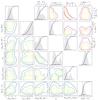 |
Fig. 8 As Fig. 7 but for the candidate BD+50 3188 in G089.0+ 04.7. |
| In the text | |
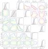 |
Fig. 9 As Fig. 7 but for the candidate HD 37424 in G180.0−01.7. |
| In the text | |
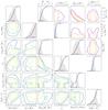 |
Fig. 10 As Fig. 7 but for the candidate HD 261393 in G205.5+ 00.5. |
| In the text | |
Current usage metrics show cumulative count of Article Views (full-text article views including HTML views, PDF and ePub downloads, according to the available data) and Abstracts Views on Vision4Press platform.
Data correspond to usage on the plateform after 2015. The current usage metrics is available 48-96 hours after online publication and is updated daily on week days.
Initial download of the metrics may take a while.