| Issue |
A&A
Volume 606, October 2017
|
|
|---|---|---|
| Article Number | A87 | |
| Number of page(s) | 13 | |
| Section | Extragalactic astronomy | |
| DOI | https://doi.org/10.1051/0004-6361/201731118 | |
| Published online | 17 October 2017 | |
Multiwavelength flaring activity of PKS 1510-089
1 Instituto de Astronomia, Geofísica e Ciências Atmosféricas, Universidade de São Paulo. Rua do Matão 1226, 05508-090 São Paulo/SP, Brazil
e-mail: This email address is being protected from spambots. You need JavaScript enabled to view it.
2 Museu de Astronomia e Ciências Afins, Ministério da Ciência, Tecnologia, Inovações e Comunicações (MAST/MCTIC), Rua General Bruce 586, 20921-030 Bairro Imperial de São Cristóvão, Rio de Janeiro, Brazil
Received: 5 May 2017
Accepted: 26 June 2017
Abstract
Aims. In this work, we analyse the multiwavelength brightness variations and flaring activity of FSRQ PKS 1510-089, aiming to constrain the position of the emission sources.
Methods. We report 7 mm (43 GHz) radio and R-band polarimetric observations of PKS 1510-089. The radio observations were performed at the Itapetinga Radio Observatory, while the polarimetric data were obtained at the Pico dos Dias Observatory. The 7 mm observations cover the period between 2011 and 2013, while the optical polarimetric observations were made between 2009 and 2012.
Results. At 7 mm, we detected a correlation between four radio and γ-ray flares with a delay of about 54 days between them; the higher frequency counterpart occurred first. Using optical polarimetry, we detected a large variation in polarization angle (PA) within two days associated with the beginning of a γ-ray flare. Complementing our data with other data obtained in the literature, we show that PA presented rotations associated with the occurrence of flares.
Conclusions. Our results can be explained by a shock-in-jet model, in which a new component is formed in the compact core producing an optical and/or γ-ray flare, propagates along the jet, and after some time becomes optically thin and is detected as a flare at radio frequencies. The variability in the polarimetric parameters can also be reproduced; we can explain large variation in both PA and polarization degree (PD), in only one of them, or in neither, depending on the differences in PA and PD between the jet and the new component.
Key words: galaxies: active / BL Lacertae objects: individual: PKS 1510-089 / radiation mechanisms: non-thermal / galaxies: jets
© ESO, 2017
1. Introduction
Blazars are active galactic nuclei (AGNs) characterized by non-thermal spectral energy distribution (SED), polarized emission, and a high level of variability, from radio frequencies to γ rays, sometimes on very short timescales (Fossati et al. 1997; Ghisellini et al. 1998; Aharonian et al. 2007). These extreme properties are believed to be a consequence of the very small angles between the relativistic jets, where the emission occurs, and the line of sight (Ghisellini & Maraschi 1989; Urry & Padovani 1995; Sambruna et al. 1996; Maraschi & Tavecchio 2003; Ghisellini & Tavecchio 2008).
The SED of blazars presents two broad features, a low-frequency component attributed to synchrotron radiation from relativistic electrons and a high-energy component that could be produced by different processes involving leptons and/or hadrons (Böttcher 2010). In the leptonic models, the high-energy emission is the result of inverse Compton (IC) interaction between the same electron/positron distribution that produces the low-energy component of the SED and low-energy photons, produced in the synchrotron process (SSC), the accretion disk, the broad line region (BLR), or the dusty torus (DT). In the hadronic models, the high-energy component of the SED is due to synchrotron radiation of the proton population, while at TeV energies, synchrotron radiation of pions and muons could predominate (Diltz et al. 2015). Both leptonic and hadronic models were able to reproduce snapshots of the SED of blazars detected by Fermi-LAT at high energies (HE), assuming equilibrium between high-energy particle injection, energy losses, and escape from the emission zone and conditions close to equipartition between electron/proton energies and magnetic fields, but the SEDs of those objects for which very high energy (VHE) was detected with Cherenkov arrays can be fitted better using hadronic models (Böttcher et al. 2013).
Considering the variability detected in the HE emission, very short doubling timescales imply a very small size for the emission region, favouring its position at the base of the relativistic jet; the low-energy photons involved in the external Compton (EC) process could then be located in the BLR (Ghisellini et al. 2010; Nalewajko et al. 2012). In that case, the high-energy γ-ray photons would be absorbed by the dense plasma via pair production, producing a high-energy cut-off in the SED (Poutanen & Stern 2010). This cut-off is in fact seen in most of the flat spectrum radio quasars (FSRQs), where strong and broad optical emission lines reveal the existence of BLR clouds (Abdo et al. 2010a), except in a few of them where VHE emission is also detected.
Multiwavelength variability and polarization properties make the location of the high-energy emission even more uncertain. In general, there seems to be a delay betweenvariabilityatdifferent frequencies; the high-frequency emission occurs first (Botti & Abraham 1988; Stevens et al. 1994, 1998; Chatterjee et al. 2008; Larionov et al. 2008; Pushkarev et al. 2010; Beaklini & Abraham 2014; Fuhrmann et al. 2014; Max-Moerbeck et al. 2014), as is expected from optical depth considerations if the emission region expands as it moves outward from the base of the relativistic jet.
On the other hand, detection of simultaneous radio and γ-ray flares together with large variations in the optical polarization angle (PA; Marscher et al. 2008, 2010; Jorstad et al. 2010; Agudo et al. 2011; Larionov et al. 2016) could imply that the IC emission originates downstream of the jet. In that case, the small sizes required by short timescale variability were explained as interaction between small turbulent regions and a standing shock (Marscher 2014; Kiehlmann et al. 2016).
The blazar PKS 1510-089, object of our study, presents most of the characteristics discussed above. With redshift z = 0.360 ± 0.002 (Thompson et al. 1990), it is one of the FSRQs that presents VHE emission, a high degree of polarization, large and fast variations in the polarization angle, and simultaneous radio and γ-ray flares. It is a core-dominated source with typical flux density at radio frequencies in the range of 1 to 4 Jy (Teräsranta et al. 2005; Algaba et al. 2011); its relativistic jet forms an angle of about 3 degrees with the line of sight (Homan et al. 2002).
PKS 1510-089 has been the target of several optical monitoring programmes (e.g. Villata et al. 1997; Raiteri et al. 1998; Romero et al. 2002) and seems to be characterized by periods of quiescence followed by large amplitude flares on timescales of several days to months. At γ rays, it was discovered as a HE source by EGRET (Hartman et al. 1999), but the existence of significant brightness variability at GeVs has only been verified since 2008, based on AGILE (D’Ammando et al. 2009) and Fermi-LAT observations (Abdo et al. 2010a), while the first detection of the source at TeV energies occurred in 2009, by H.E.S.S. telescopes (H.E.S.S. Collaboration et al. 2013).
Multiwavelength campaigns were organized during HE activity (Orienti et al. 2013; Aleksić et al. 2014; MAGIC Collaboration et al. 2017; Castignani et al. 2017) and monitoring at radio frequencies are performed on a regular basis by different programmes, e.g. F-GAMMA (Fermi-GST AGN Multi-Frequency Monitoring Alliance), GASP (GLAST-AGILE Support Program), UMRAD (University of Michigan Radio Observatory), OVRO (Owens Valley Radio Observatory) 40-m telescope monitoring at 15 GHz.
It has long been known that PKS 1510-089 is a highly polarized source at optical wavelengths (Appenzeller & Hiltner 1967; Moore & Stockman 1984). At radio wavelengths, VLBA maps show the existence of a highly polarized and variable core (Jorstad et al. 2005, 2007; Linford et al. 2011), variability that seems to be correlated with gamma-ray events (Marscher et al. 2010; Sasada et al. 2011; Orienti et al. 2013).
In 2011, the γ-ray light curve obtained from Fermi-LAT observations showed the existence of successive flares (Foschini et al. 2013; Aleksić et al. 2014), while the radio flux started a continuous increase some weeks after the first γ-ray flare (Nestoras et al. 2011; Orienti et al. 2011, 2013; Beaklini et al. 2011a). At R band, the light curve obtained by Bonning et al. (2012) using the SMARTS telescopes (Small and Moderate Aperture Research Telescope System) did not show outbursts simultaneous with the γ-ray flares (Bonning et al. 2012). However, the existence of many gaps during this period could hide the existence of any correlation.
Marscher et al. (2010) claimed the detection of a rotation higher than 700° in PA at R band before the occurrence of a γ-ray flare observed by Fermi-LAT (Abdo et al. 2010b), presenting a similar behaviour to that detected in BL Lac (Marscher et al. 2008). The authors interpreted it as a consequence of the existence of a helical magnetic field in the path of a new jet component before it crosses an optically thick core, located far from the central engine. However, the detection of that large continuous rotation is still under debate (Sasada et al. 2011; Jermak et al. 2016).
In 2009 we started a monitoring programme of some bright blazars at 43 GHz (7 mm) and at optical polarimetry. PKS 1510-089 was included in our optical sample, but not in the radio sample as it was considered a weak source to be observed with a S/N that was good enough for variability analysis. However, after the detection of gamma-ray flares in 2011 (Saito et al. 2013; Foschini et al. 2013), we followed the increase in the radio flux density, also detected by other authors (Beaklini et al. 2011a,b; Nestoras et al. 2011; Orienti et al. 2011), and then we started to monitor PKS 1510-089 regularly also at 7 mm.
In this work we present the results of these observational efforts. The data were compared with those available in the literature at other wavelengths, including γ-ray observations from Fermi-LAT. Special attention was given to the epochs of intense activity in the form of strong flares. In Sect. 2 we describe the observational programme and the data analysis. The results from our observations are presented in Sect. 3, and they are discussed and compared with other data sets available the literature in Sect. 4. Finally, in Sect. 5 we present our conclusions.
2. Observations
2.1. Radio observations
The 7 mm observations of PKS 1510-089 began in January 2011 after the detection of γ-ray flares by Fermi-LAT, and continued monthly until April 2013. They were made at the Itapetinga Radio Observatory, in Atibaia, São Paulo, Brazil. The radiotelescope consists of a 13.7 m radome enclosed antenna and a room temperature K-band receiver, with a 1 GHz double sideband and a noise temperature of about 700 K, which provides a 2.4 arcmin HPBW. For instrumental calibration we used a room temperature load and a noise source of known temperature in a procedure that takes into account radome and atmospheric absorption (Abraham & Kokubun 1992). SgrB2 Main, an HII complex close to the galactic centre, was used as flux calibrator.
We used the scan method (on-the-fly) for the observations. Each scan lasted 20 s, was centred at the source coordinates, and had an amplitude of 30 arcmin in elevation or azimuth. As we were observing a point source, we used the scans in both directions to verify the pointing accuracy. During one scan, we measured 81 uniformly spaced points; each observation consisted of 30 scans and the instrumental calibration was performed every 30 min. For SgrB2 Main, which has an angular size larger than the beam width, the scans were made along the right ascension coordinate. On a typical day, we performed between 18 and 20 observations of PKS 1510-089.
2.2. Optical polarimetry
Optical polarimetric observations were carried out between 2009 and 2012 using the 0.6 m Boller & Chivens IAG/USP telescope at Pico dos Dias Observatory (OPD, Brazópolis, Brazil)1 and an imaging polarimeter, IAGPOL (Magalhaes et al. 1996), working in linear polarization mode with a standard R-band filter. The polarimeter consists of a rotatable achromatic half-wave retarder, followed by a calcite Savart plate. This configuration provides two images of each object in the field with orthogonal polarizations, separated by 1 mm or 25.5 arcsec at the telescope focal plane. The simultaneous detection of the two beams allows observations under non-photometric conditions and has the advantage that the sky polarization is practically cancelled out. The observations were performed over a few consecutive nights on a monthly basis, with several observations during each night.
Throughout the years of monitoring, we used two different CCDs: a 1024 × 1024 pixel CCD of 24 microns/pixel and a 2048 × 2048 pixel CCD of 13.5 microns/pixel, both providing a field of view of about 10′ × 10′ (0.67′′/pixel and 0.38′′/pixel, respectively). Each polarization measurement was obtained from eight different wave plate positions separated by  , consuming a mean total integration time of about 30 min, depending on the quality of the night The images were reduced with IRAF2 usual routines for bias and flat field corrections. The PCCDPACk package (Pereyra 2000) was used to calculate the polarization, its parameters, and errors based on Serkowski (1974a,b). The conversion of the polarization position angle PA to the equatorial system was made using observations of polarized standard stars in each night (HD 298383, HD 111579, and HD 155197). The lack of instrumental polarization was checked through the observation of unpolarized standard stars (HD 94851, WD 1620, and HD 94851).
In an imaging polarimeter like IAGPOL, the total flux density can be recovered by adding both polarimetric components. However, this procedure is reliable only for photometric nights. In order to check the quality of the data obtained with this method, we used the public light curves from the Yale/SMARTS monitoring programme (Bonning et al. 2012), available from the webpage of the project3. Comparing coincident observations between our daily averaged data and those of the SMARTS programme, we found a maximum error of 30% in the total flux, a value that we assume as the error for of all our flux density measurements. Obtaining photometric information from polarimetric data, even with large error bars, allows us to compare total flux and polarization simultaneously.
SMARTS data were also used to compare our polarimetric results with a better sampled optical light curve. Blazars at declinations smaller than 20 degrees from the list of sources monitored by the Fermi telescope have been observed by the Yale/SMARTS consortium since 2008, with a 1.3 m telescope at CTIO and the dual-channel imager ANDICAM (DePoy et al. 2003). By using a dichroic to feed an optical CCD and an IR detector, the instrument can obtain simultaneous data in the B, V, R, J, and K bands. For this work, we selected only the R band because it is the same used in our polarimetric observations. The Yale/SMARTS observation of each object are obtained at least once every three days. To compute the calibrated flux densities used throughout this work, we considered a galactic extinction of AR = 0.258 (Schlegel et al. 1998).
Radio flux density obtained in this work.
2.3. Fermi data
The Fermi Space Observatory provides daily light curves of blazars, including PKS 1510-089. The telescope was launched in 2008 to explore the Universe in the energy range of 10 keV to 300 GeV. In particular, it carries the Large Area Telescope (LAT) as the main instrument, which allows the observation of the entire sky every three hours. A complete description of the LAT instrument and its operation and can be found in Atwood et al. (2009). In this work, we used the Fermi monitoring data available in the Fermi Light Curve page4.
We chose the largest energy band width (Band 3, >100 MeV) to compare with the radio and the polarimetric light curves. In order to smooth the light curve and to compare it with the long variability trend at radio wavelengths, the γ-ray data were re-sampled in five-day bins.
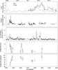 |
Fig. 1 From top to bottom: 7 mm radio light curve obtained in this work together with the 7 mm peak flux density of VLBA images obtained from the VLBI-BU BLAZAR monitoring programme; R-band photometry from SMARTS (Bonning et al. 2012); Fermi-LAT γ-ray light curve for energies >100 MeV, binned in five-day intervals (Abdo et al. 2009a,b, 2010c); R-band polarization degree and position angle obtained in this work. |
3. Results
We present the observed 7 mm flux density of PKS 1510-089 in Table 1 and the R-band polarimetric results in Table A.1. Since there is a 180° ambiguity in PA, we selected the values that minimize the difference between consecutive angle measurements, allowing both clockwise and anticlockwise rotations. In Fig. 1 from top to bottom we show the 7 mm Itapetinga light curve together with the total peak intensity of VLBA images obtained from the VLBA-BU-BLAZAR Program5: the R-band light curve from SMARTS (Bonning et al. 2012), the Fermi-LAT γ-ray flux at energies higher than 100 MeV (Abdo et al. 2009a,b), and our measurements of PD and PA at R band. The γ-ray data were binned in five-day intervals to smooth the light curve, allowing a better comparison with our 7 mm results.
3.1. The 7 mm light curve
As can be seen in Fig. 1, the source presented small fluctuations at 7 mm during the first semester of our monitoring programme, with a mean flux density of (2.6 ± 0.5) Jy, not an unusual level for this object (Teräsranta et al. 2005; Algaba et al. 2011). In the second semester of 2011, about 50 days after the occurrence of a γ-ray flare detected by Fermi-LAT on 1 July 2011, the brightness started to increase gradually (Beaklini et al. 2011a,b; Nestoras et al. 2011; Orienti et al. 2011), reaching the maximum flux density of (8.2 ± 0.9) Jy, never before detected in this source. It should be noted that this exceptional increase lasted almost one year, although with some variability, while the decline was faster, taking only two months. Similar behaviour was found by the F-GAMMA monitoring programme at frequencies ranging from 2.6 GHz to 142 GHz (Orienti et al. 2013) and in data obtained by the Metsähovi Observatory at 37 GHz (Aleksić et al. 2014), including the maximum flux density but taking into account that there is a delay between the different frequencies, as is discussed in the next section, and that these observations covered a shorter period of time, missing the decaying phase. During this period of time, several γ-ray flares were detected by Fermi-LAT, some of them exceeding the γ-ray flux of 10-5 ph cm-3 s-1, with a doubling time of the order of 20 min (Foschini et al. 2013).
Comparing our 7 mm light curve with the corresponding VLBA peak intensity data, in the top panel of Fig. 1 we see that the latter, which corresponds to the core emission, reached its maximum value before our single-dish data, implying that after 2012 the jet components included in our single-dish detection contributed considerably to the total flux density.
We tried to find a correlation between the γ-ray and 7 mm light curves, assuming that the continuous increase in flux density was the result of the superposition of radio flares associated with the high-energy events. Because of the difference in flare duration at the two frequencies, it was not possible to find a correlation using statistical techniques, even those designed for unevenly sampled data as the Discrete Correlation Function (Edelson & Krolik 1988). Instead, we confirmed the correlation using the peaks of both light curves. For γ-rays, we choose as peaks the points where the flux density is three times higher than the rms of the quiescent phase; when several flares occurred in a short time interval, we used the mean epoch of the group. For radio variability, the superposition of flares made the identification of the corresponding peaks more difficult; we selected the peaks as the local maxima in the light curve. In Fig. 2, the excellent correlations between the flares at the two frequencies can be seen; the radio flares are delayed by about 54 days relative to the γ-ray flares. In Fig. 3 we present the 7 mm and γ-ray light curves; the 7 mm data is shifted by –54 days to show the correspondence between the different flares.
3.2. Polarimetry
The polarimetric data, shown in the bottom panels of Fig. 1, presented different patterns during 2009, including large variations in PA and/or PD in daily timescales and sometimes during the same night.
Between 31 March 2009 and 1 April, five days after the occurrence of a γ-ray flare and the detection of VHE emission by H.E.S.S. (H.E.S.S. Collaboration et al. 2013), there was a change of about 40° in PA in the clockwise direction and a small increase in PD.
Between 20 April and 22 April 2009, coincident with the beginning of a γ-ray flare (Abdo et al. 2010b) and the ejection of a new superluminal component (Marscher et al. 2010), PA changed by 65° in the anticlockwise direction and PD decrease from 7.7% to 4.7%, going back to 8.5% on 23 April, without any significant change in PA. The coincidence between the γ-ray intensity and variations in PA during this flare can be seen in more detail in Fig. 4.
From 20 May to 22 May 2009, PD increased from 1% to 7.4% without large changes in PA; by the end of June the source was depolarized6, going back to 6% PD in July.
Between 12 April and 14 April 2010 the source was depolarized, while one month later it reached the maximum measured value of PD (11.02% ± 0.05%) after the occurrence of a γ-ray flare with a doubling timescale of ~ 0.3 h (Foschini et al. 2013).
In 2011, when the radio flux density increased simultaneously with the occurrence of several γ-ray flares, we found only small amplitude variations in PD and PA, which might have been a consequence of our limited sampling since most of the γ-ray activity occurred when PKS 1510-089 could not be observed at night.
In Fig. 5 we show our R-band polarization data in the Q/Ip × U/Ip plane, which has the advantage of being independent of any criterion used to solve the 180° multiplicity. Owing to the trigonometric relation between PA and the Stokes parameters, a continuous rotation of PA should produce consecutive changes of quadrants in this plane, as argued by Sasada et al. (2011). In our data, we detected large changes during or close to the occurrence of flares, and small fluctuations at other epochs.
We show in Fig. 6 the relation of PD with magnitude during the polarimetric monitoring. We found a Pearson coefficient correlation of r = 0.5 with the full data set. A positive correlation r = 0.8 was obtained by Ikejiri et al. (2011), restricted to the observations where the source was brighter than 15.5 mag in V-band.
Other polarimetric observations in 2009 at R band (Marscher et al. 2010; Jermak et al. 2016) and at V band (Sasada et al. 2011) showed a variable behaviour for PD similar that found in our work, although with even higher maximum values. The behaviour of PA was also similar, except for the addition of 180° and the sense of rotation, which was always in the same anticlockwise direction in Marscher et al. (2010), and in both directions in Sasada et al. (2011) and Jermak et al. (2016).
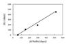 |
Fig. 2 Correlation between the time of occurrence of radio and γ-ray flares. Zero corresponds to the first γ-ray flare, on 01 Jul. 2011. The dates of the other γ-ray flares are 24 Oct. 2011, 21 Feb. 2012, and 23 Sept. 2012. The radio peaks correspond to 28 Aug. 2011, 29 Nov. 2011, 22 Apr. 2012, and 30 Nov. 2012. |
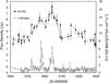 |
Fig. 3 Light Curves of PKS 1510-089 at 7 mm (this work, black dots) and at γ rays (band 3 data from Fermi-LAT, white dots). The 7 mm light curve is shifted by –54 days. |
4. Discussion
4.1. The 7 mm light curve
We have shown that what looked like a single extremely strong radio flare at 7 mm in our single-dish observations, starting during the second semester of 2011 and ending one year later, is better interpreted as the superposition of three flares delayed with relation to the respective γ-ray flares. A similar delay was found for a fourth isolated flare, observed at 7 mm on 30 November 2012, which we believe is the counterpart of the γ-ray flare of 23 September 2012.
The existence of a correlation and delays between the variabilities favours the scenario of a common origin of γ-ray and radio flares, like that proposed by the shock-in-jet models and their generalizations (Marscher & Gear 1985; Marscher 1990; Marscher et al. 1992; Hughes et al. 1985; Stevens et al. 1996; Türler et al. 1999; Sokolov et al. 2004). In these models, electrons are accelerated to ultra-relativistic energies in a shock, and as they propagate along the jet they emit synchrotron radiation at low frequencies producing high-energy photons by the inverse Compton process. The delay is explained if the shock is formed close to the core, where the jet is optically thick to radio frequencies, but transparent to high energies, so that photons from either the BL region or DT could produce the observed high-energy emission (Aleksić et al. 2014).
Other evidence confirms this interpretation. First, by comparing the single-dish 7 mm light curve with the flux density of the VLBA core at the same frequency in Fig. 1, we verify that the single-dish flux density was always larger during flares, implying that when the new components become optically thin, they have already left the core. In fact, Orienti et al. (2013) identified a new component in the 15 GHz VLBA images, ejected from the core in 2012 (July or October) at a velocity of (0.92 ± 0.35) mas yr-1; after our measured delay of 54 days, when the component became optically thin at 7 mm, its distance to the core was (0.14 ± 0.05) mas, being resolved by the 0.1 mas VLBA beam (Marscher et al. 2012). The formation of new components associated with γ-ray flares was also confirmed by inspection of the 7 mm VLBA images obtained by the VLBA-BU-BLAZAR programme, which also showed the polarized flux.
Comparing our radio light curve with those at other frequencies from the F-GAMMA, GASP, and OVRO programmes (Orienti et al. 2013; Aleksić et al. 2014) at the same epochs, we can see a compatible behaviour. Analysing the very well-sampled 15 GHz and 22 GHz light curves obtained by Orienti et al. (2013), we can also see a sharp increase in flux density during the second semester of 2011, which seems to have occurred with a delay of approximately 50 and 35 days, respectively, relative to our 43 GHz data. At 86 GHz and 142 GHz, the light curves show a maximum very close to the second γ-ray flare in our Fig. 2, indicating that they are possibly associated.
We also verified that in the 22 GHz light curves presented by Orienti et al. (2013) using VLBI Exploration of Radio Astrometry (VERA), there was no difference between the single-dish flux density and that of the VLBI core, which can be understood considering that new components became optically thin at this frequency 90 days after the γ-ray flare, at a distance of 0.22 mas from the core, not being resolved by the (1.5 × 1.0) mas VERA beam.
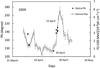 |
Fig. 4 Abrupt variation in PA simultaneous with the beginning of a γ-ray flare in PKS 1510-089 during April 2009. |
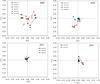 |
Fig. 5 Q × U plane normalized by Ip during four different years of our monitoring. |
Aleksić et al. (2014) presented the spectral evolution of PKS 1510-089 over 80 days, from MJD 55 954 (01/27/2012) to MJD 56 034 (04/16/2012); in Fig. 7a we show these spectra including our 43 GHz data. We can see that the 43 GHz data fitted the overall SED only at the first epoch, with the flux density starting to increase continuously afterwards, as expected if a new component was formed, which remained optically thick at low frequencies and started to become optically thin at 43 GHz. In Fig. 7b we show the SED at earlier epochs than those presented in Fig. 7a, with our 43 GHz data superposed to those presented in Orienti et al. (2013). The first epoch corresponds to the quiescent period of PKS 1510-089, with a smooth and almost flat SED. On MJD 55 862 the SED presented two different peaks, at 22 GHz and 86 GHz, with flux densities close to their maximum values, which we can interpret as evidence of the contribution of two components. The low-frequency peak corresponds to the first flare in our Fig. 2, becoming optically thin 35 days after 43 GHz, as mentioned before, while the high-frequency peak corresponds to the component formed during the second γ-ray flare, on MJD 55 858. It is the high-frequency component that increased the flux density at 43 GHz in MJD 55 917.
A similar delay between radio and γ-ray flares seems to have occurred in 2009 (Marscher et al. 2010), but it was not covered by our radio observations. At that epoch, three groups of γ-rays flares were observed, separated by about 50 days, with a sharp increase in flux density at 15 GHz, 37 GHz, and 230 GHz coinciding with the last of the flares. Taking into account the time delay between radio and γ-ray emission, we believe that – instead of a coincidence with the last flare – the increase in the radio flux density could be attributed to a delayed synchrotron emission from the previous one. In Fig. 9 we present the radio light curve obtained by Marscher et al. (2010) shifted by the same delay adopted in Fig. 3 (54 days). With this displacement in time, the beginning of the increase in radio flux density seems to be associated with the first γ-ray flare. Naturally, flare delays in 2009 and 2011 do not need to have the same value, but as can be seen, a delay similar to that in 2011 could also explain the 2009 variability.
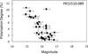 |
Fig. 6 Relation between PD and R-band magnitude in PKS 1510-089 between 2009 and 2012. |
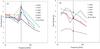 |
Fig. 7 Radio spectra of PKS 1510-089 during several epochs with 7 mm data (black dots) obtained in this work superposed with Aleksić et al. (2014) observations at (a) and with Orienti et al. (2013) observations at (b). |
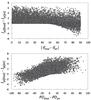 |
Fig. 8 Difference between polarized fluxes before and after the formation of a new component as a function of the difference in PA of the new and old component (upper panel) and difference in PD before and after the formation of the new component (lower panel). |
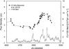 |
Fig. 9 Light curves of PKS 1510-089 at 37 GHz (black dots) obtained by Marscher et al. (2010) and at γ-rays (band 3 data from Fermi-LAT, white dots). The radio light curve was shifted by 54 days, the same time delay as in Fig. 3. |
4.2. Stokes parameters of a new component
The formation of new jet components can also explain the behaviour of the optical polarization, which shows, during flares, variability in both PA and PD, in only one of them, or in neither of them. To understand this behaviour, let us consider as in Holmes et al. (1984), the Stokes parameters for two components; in our case, before and after the formation of a new component. We represent the jet as a single structure before the formation of the new component, with Stokes parameters ![Mathematical equation: \begin{eqnarray} \label{eq1} &&Q_{\rm jet} = I_{\rm p(jet)}\cos{2 \theta_{\rm jet}}, \\[3mm] \label{eq2} &&U_{\rm jet} = I_{\rm p(jet)}\sin{2 \theta_{\rm jet}}, \end{eqnarray}](/articles/aa/full_html/2017/10/aa31118-17/aa31118-17-eq48.png) where θjet is the PA and Ip(jet) is the total polarized flux density before the formation of the new component. The Stokes parameters of the source after the ejection (Qfinal,Ufinal, and Ip(final)) can be written as
where θjet is the PA and Ip(jet) is the total polarized flux density before the formation of the new component. The Stokes parameters of the source after the ejection (Qfinal,Ufinal, and Ip(final)) can be written as  where Qnew and Unew are the Stokes parameters of the new component. Solving these equations for the total polarization angle θfinal and for the polarized intensity Ip(final), we have
  We investigate the possibility that Ip(final)<Ip(jet) simultaneously with a large change in PA, as detected during the γ-ray flare of April 2009: Ip(jet) = (0.18 ± 0.07) mJy and θjet = −59° ± 2° on 20 April, and Ip(final) = (0.08 ± 0.02) mJy and θfinal = + 11° ± 2° on 22 April. From Eq. (8), this condition is satisfied if
  (9)or
(9)or  (10)We used Eqs. (6) to (8) to estimate the polarimetric properties of the ejected component and found
  and Ip(new) = (0.23 ± 0.10) mJy, resulting in (θnew−θjet) = 83° ± 4°, in agreement with the requirement of Eq. (10).
Different value of PA in our data after their combination with data from the literature.
Based on Eqs. (6) to (8), we also checked the incidence rate of variations in PA and PD after the ejection of a new component, simulating different combinations between PA, PD, and total flux of the jet and of the new component. We used a uniform distribution of random values for the intensities (between 0 and 7 mJy), PAs (between 0° and 180°), and PDs (between 0 and 100%). In Fig. 8 (top) we present (Ip(final)−Ip(jet)) as a function of Δθ = (θnew−θjet) and verify that the polarized flux density can indeed decrease after the formation of a new polarized component if Eq. (10) is satisfied. In Fig. 8 (bottom) we present (Ip(final)−Ip(jet)) as a function of (PDfinal−PDjet), which shows that if the polarized flux density decreases after the formation of the new component, PDfinal will be lower than PDjet. We also did simulations using a normal instead of a uniform distribution for the total flux densities, PAs, and PDs, and the results did not change significantly, indicating that the PA combination is the most important variable to obtain PAfinal−PAjet.
The existence of both large and small changes in PD with the same probability, also explains γ-ray flares without any corresponding change in PA or PD, as reported by Paliya et al. (2015) for an extremely bright γ-ray flare observed during 2014 in the FRSQ 3C 279. Those authors also pointed out that such behaviour can be evidence of a superposition of multiple components. They are also in agreement with the first year results of the Robotic Polarimetric in Crete (RoboPol), a monitoring programme of an unbiased sample of γ-ray bright blazars, which suggest that the highest amplitude γ-ray flares are correlated with rotations in PA (Blinov et al. 2015).
The results of our simulations are different from those reported by Kiehlmann et al. (2013) because they assumed variability due to random effects, used a large number of components (30), and attributed random values for Q and U instead of intensity, PD, and PA, as in our case. The analysis was carried out based on a sample with a regular small time interval of three days and, as was also pointed by the authors, poorer sampled light curves can introduce large artificial rotations.
4.3. Optical PA variability
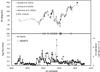 |
Fig. 10 Top: PA variability combining the results obtained in this work with those of Marscher et al. (2010), Sasada et al. (2011), and Jermak et al. (2016). Bottom: SMARTS R band and Fermi-LAT light curves. Vertical marks in the time axis represent the epochs in which rotations of more than 50° were detected in intervals of one day. |
As pointed out by Kiehlmann et al. (2016), the existence of gaps in the observations compromises the solution of the 180° multiplicity PA. Attempting to better constrain the PA variability, we combined the polarimetric data reported by Marscher et al. (2010), Sasada et al. (2011), Jermak et al. (2016), and our own data, and applied as a criterion to keep the smallest variation in PA during successive epochs, allowing rotation in both clockwise and anticlockwise senses.
The resulting PAs for our data are presented in Table 2 and the behaviour of PA including all the data are shown in Fig. 10. We can see that the largest jumps in PA coincided with the occurrence of optical and/or γ-ray flares, after which PA tended to return to its previous value. The maximum rotation during this time interval was less than 400°, in agreement with Sasada et al. (2011) and Jermak et al. (2016). Figure 10, with all data combined, shows in more detail the oscillations associated with the occurrence of optical and/or γ-ray flares.
5. Conclusions
In this paper we presented 7 mm single-dish observations of PKS 1510-089 covering the period January 2011 to September 2013 and R-band polarimetric observations at several epochs between March 2009 and May 2012. The long coverage of the 7 mm light curve allowed us to correlate four γ rays with radio flares and measure a delay of about 54 days between them, with the γ-ray emission occurring first. This result shows that sometimes the simultaneity between flares at the two frequencies can be a consequence of coincidence between the delay timescales and the rate of occurrence of the flares.
A comparison between the measured single-dish 7 mm flux density and the VLBI core emission at the same wavelength shows that the components responsible for the flares had already left the core when they become optically thin, although this was not the case at lower frequencies. These results are a consequence of the apparent velocity of the components, the time delay between gamma and radio flares, and the resolution of the different VLBI arrays used in the observations.
We detected a large rotation (65°) in R-band PA simultaneously with the start of a γ-ray flare in April 2009. Combining our observations with data from the literature, we verified that this simultaneity also occurred in other γ-ray flares. We showed that the behaviour of the polarization variability, which included sudden large variations in PA and PD, in only one of them, or in neither of them during flares can be explained by the superposition of the jet emission and that of a new component.
Operated by the Laboratório Nacional de Astrofísica (LNA/MCTIC).
IRAF is distributed by the National Optical Astronomy Observatory, which is operated by the Association of Universities for Research in Astronomy, Inc., under cooperative agreement with the National Science Foundation
We assumed the boundary definition of 3% by Angel & Stockman (1980) to classify AGNs as polarized.
Acknowledgments
We are grateful to the Brazilian research agencies FAPESP and CNPq for financial support (FAPESP Projects: 2008/11382-3 and 2014/07460-0). This study makes use of 43 GHz VLBA data from the VLBA-BU Blazar Monitoring Program (VLBA-BU-BLAZAR; http://www.bu.edu/blazars/VLBAproject.html), funded by NASA through the Fermi Guest Investigator Program. The VLBA is an instrument of the National Radio Astronomy Observatory. The National Radio Astronomy Observatory is a facility of the National Science Foundation operated by Associated Universities, Inc. This paper has made use of up-to-date SMARTS optical/near-infrared light curves that are available at www.astro.yale.edu/smarts/glast/home.php. This research has made use of data from the MOJAVE database that is maintained by the MOJAVE team (Lister et al. 2009).
References
- Abdo, A. A., Ackermann, M., Ajello, M., et al. 2009a, ApJ, 700, 597 [NASA ADS] [CrossRef] [Google Scholar]
- Abdo, A. A., Ackermann, M., Ajello, M., et al. 2009b, ApJ, 707, 1310 [NASA ADS] [CrossRef] [Google Scholar]
- Abdo, A. A., Ackermann, M., Ajello, M., et al. 2010a, ApJ, 710, 1271 [NASA ADS] [CrossRef] [Google Scholar]
- Abdo, A. A., Ackermann, M., Agudo, I., et al. 2010b, ApJ, 721, 1425 [NASA ADS] [CrossRef] [Google Scholar]
- Abdo, A. A., Ackermann, M., Ajello, M., et al. 2010c, ApJ, 715, 429 [NASA ADS] [CrossRef] [Google Scholar]
- Aharonian, F. A., Akhperjanian, A. G., Bazer-Bachi, A. R., et al. 2007, ApJ, 664, L71 [Google Scholar]
- Abraham, Z., & Kokubun, F. 1992, A&A, 257, 831 [NASA ADS] [Google Scholar]
- Agudo, I., Jorstad, S., Marscher, A. P., Larionov, V. M., & Gómez, J. L. 2011, ApJ, 726, L13 [NASA ADS] [CrossRef] [Google Scholar]
- Aleksić, J., Ansoldi, S., Antonelli, L. A., et al. 2014, A&A, 569, A46 [NASA ADS] [CrossRef] [EDP Sciences] [Google Scholar]
- Algaba, J. C., Gabuzda, D. C., & Smith, P. S. 2011, MNRAS, 411, 85 [NASA ADS] [CrossRef] [Google Scholar]
- Angel, J. R. P., & Stockman, H. S. 1980, ARA&A, 18, 321 [NASA ADS] [CrossRef] [Google Scholar]
- Appenzeller, I., & Hiltner, W. A. 1967, ApJ, 149, L17 [NASA ADS] [CrossRef] [Google Scholar]
- Atwood, W. B., Abdo, A. A., Ackermann, M., et al. 2009, ApJ, 697, 1071 [NASA ADS] [CrossRef] [Google Scholar]
- Beaklini, P. P. B., & Abraham, Z. 2014, MNRAS, 437, 489 [NASA ADS] [CrossRef] [Google Scholar]
- Beaklini, P. P., Abraham, Z., & Dominici, T. P. 2011a, ATel, 3799, 1 [NASA ADS] [Google Scholar]
- Beaklini, P. P., Dominici, T. P., & Abraham, Z. 2011b, ATel, 3523, 1 [NASA ADS] [Google Scholar]
- Blinov, D., Pavlidou, V., Papadakis, I., et al. 2015, MNRAS, 453, 1669 [NASA ADS] [CrossRef] [Google Scholar]
- Bonning, E., Urry, C. M., Bailyn, C., et al. 2012, ApJ, 756, 13 [NASA ADS] [CrossRef] [Google Scholar]
- Böttcher, M. 2007, Ap&SS, 309, 95 [NASA ADS] [CrossRef] [Google Scholar]
- Böttcher, M., 2010, in Proc. of the Workshop Fermi meets Jansky: AGN in Gamma Rays, eds. T. Savolainen, E. Ros, R. W. Porcas, & J. A. Zensus (Bonn: Max-Plank-Institut fürRadioastronomy), 41 [Google Scholar]
- Böttcher, M., Reimer, A., Sweeney, K., & Prakash, A. 2013, ApJ, 768, 54 [NASA ADS] [CrossRef] [Google Scholar]
- Botti, L. C. L., & Abraham, Z. 1988, AJ, 96, 465 [NASA ADS] [CrossRef] [Google Scholar]
- Castignani, G., Pian, E., Belloni, T. M., et al. 2017, A&A, 601, A30 [NASA ADS] [CrossRef] [EDP Sciences] [Google Scholar]
- Chatterjee, R., Jorstad, S. G., Marscher, A. P., et al. 2008, ApJ, 689, 79 [NASA ADS] [CrossRef] [Google Scholar]
- D’Ammando, F., Pucella, G., Raiteri, C. M., et al. 2009, A&A, 508, 181 [NASA ADS] [CrossRef] [EDP Sciences] [Google Scholar]
- DePoy, D. L., Atwood, B., Belville, S. R., et al. 2003, Proc. SPIE, 4841, 827 [NASA ADS] [CrossRef] [Google Scholar]
- Diltz, C., Böttcher, M., & Fossati, G. 2015, ApJ, 802, 133 [NASA ADS] [CrossRef] [Google Scholar]
- Edelson, R., & Krolik, J. 1988, ApJ, 333, 646 [NASA ADS] [CrossRef] [Google Scholar]
- Foschini, L., Bonnoli, G., Ghisellini, G., et al. 2013, A&A, 555, A138 [NASA ADS] [CrossRef] [EDP Sciences] [Google Scholar]
- Fossati, G., Celotti, A., Ghisellini, G., & Maraschi, L. 1997, MNRAS, 289, 136 [NASA ADS] [CrossRef] [Google Scholar]
- Fuhrmann, L., Larsson, S., Chiang, J., et al. 2014, MNRAS, 441, 1899 [NASA ADS] [CrossRef] [Google Scholar]
- Ghisellini, G., & Maraschi, L. 1989, ApJ, 340, 181 [NASA ADS] [CrossRef] [Google Scholar]
- Ghisellini, G., & Tavecchio, F. 2008, MNRAS, 387, 1669 [NASA ADS] [CrossRef] [Google Scholar]
- Ghisellini, G., Celotti, A., Fossati, G., Maraschi, L., & Comastri, A. 1998, MNRAS, 301, 451 [NASA ADS] [CrossRef] [Google Scholar]
- Ghisellini, G., Tavecchio, F., Ghirlanda, G., Maraschi, L., & Celotti, A. 2010, MNRAS, 402, 497 [NASA ADS] [CrossRef] [Google Scholar]
- H.E.S.S. Collaboration, Abramowski, A., Acero, F., et al. 2013, A&A, 554, A107 [NASA ADS] [CrossRef] [EDP Sciences] [Google Scholar]
- Holmes, P. A., Brand, P. W. J. L., Impey, C. D., et al. 1984, MNRAS, 211, 497 [NASA ADS] [CrossRef] [Google Scholar]
- Homan, D. C., Wardle, J. F. C., Cheung, C. C., Roberts, D. H., & Attridge, J. M. 2002, ApJ, 580, 742 [NASA ADS] [CrossRef] [Google Scholar]
- Hartman, R. C., Bertsch, D. L., Bloom, S. D., et al. 1999, ApJS, 123, 79 [NASA ADS] [CrossRef] [Google Scholar]
- Hughes, P. A., Aller, H. D., & Aller, M. F. 1985, ApJ, 298, 301 [NASA ADS] [CrossRef] [Google Scholar]
- Ikejiri, Y., Uemura, M., Sasada, M., et al. 2011, PASJ, 63, 639 [NASA ADS] [Google Scholar]
- Jermak, H., Steele, I. A., Lindfors, E., et al. 2016, MNRAS, 462, 4267 [NASA ADS] [CrossRef] [Google Scholar]
- Jorstad, S. G., Marscher, A. P., Mattox, J. R., et al. 2001, Ap&SS, 134, 181 [Google Scholar]
- Jorstad, S. G., Marscher, A. P., Lister, M. L., et al. 2005, AJ, 130, 1418 [NASA ADS] [CrossRef] [Google Scholar]
- Jorstad, S. G., Marscher, A. P., Stevens, J. A., et al. 2007, AJ, 134, 799 [NASA ADS] [CrossRef] [Google Scholar]
- Jorstad, S. G., Marscher, A. P., Larinov, V. M., et al. 2010, ApJ, 715, 362 [NASA ADS] [CrossRef] [Google Scholar]
- Kiehlmann, S., Savolainen, T., Jorstad, S. G., et al. 2013, EPJ Web Conf., 61, 06003 [Google Scholar]
- Kiehlmann, S., Savolainen, T., Jorstad, S. G., et al. 2016, A&A, 590, A10 [NASA ADS] [CrossRef] [EDP Sciences] [Google Scholar]
- Larionov, V. M., Jorstad, S. G., Marscher, A. P., et al. 2008, A&A, 492, 389 [NASA ADS] [CrossRef] [EDP Sciences] [Google Scholar]
- Larionov, V. M., Jorstad, S. G., Marscher, A. P., & Smith, P. S. 2016, Galaxies, 4, 43 [NASA ADS] [CrossRef] [Google Scholar]
- Linford, J. D., Taylor, G. B., Romani, R. W., et al. 2011, ApJ, 726, 16 [NASA ADS] [CrossRef] [Google Scholar]
- Lister, M. L., Cohen, M. H., Homan, D. C., et al. 2009a, AJ, 138, 1874 [NASA ADS] [CrossRef] [Google Scholar]
- Lister, M. L., Aller, H. D., Aller, M. F., et al. 2009b, AJ, 137, 3718 [NASA ADS] [CrossRef] [Google Scholar]
- Magalhaes, A. M., Rodrigues, C. V., Margoniner, V. E., Pereyra, A., & Heathcote, S. 1996, in Polarimetry of the Interstellar Medium, eds. W. G. Roberge, & D. C. B. Whittet (San Francisco: ASP), ASP Conf. Ser. 97, 118 [Google Scholar]
- MAGIC Collaboration, Ahnen, M. L., Ansoldi, S., et al. 2017, A&A, 603, A29 [NASA ADS] [CrossRef] [EDP Sciences] [Google Scholar]
- Maraschi, L., & Tavecchio, F. 2003, ApJ, 593, 667 [NASA ADS] [CrossRef] [Google Scholar]
- Marscher, A. P. 1990, in Parsec-Scale Radio Jets, eds. J. A. Zensus, & T. J. Pearson (Cambridge: Cambridge Univ. Press), 236 [Google Scholar]
- Marscher, A. P. 2014, ApJ, 780, 87 [NASA ADS] [CrossRef] [Google Scholar]
- Marscher, A. P., & Gear, W. K. 1985, ApJ, 298, 114 [NASA ADS] [CrossRef] [Google Scholar]
- Marscher, A. P., Gear, W. K., & Travis, J. P. 1992, Variability of Blazars (Cambridge: Cambridge University Press), 85 [Google Scholar]
- Marscher, A. P., Jorstad, S. G., D’Arcangelo, F. D., et al. 2008, Nature, 452, 966 [NASA ADS] [CrossRef] [PubMed] [Google Scholar]
- Marscher, A. P., Jorstad, S. G., Larionov, V. M., et al. 2010, ApJ, 710, L126 [NASA ADS] [CrossRef] [Google Scholar]
- Marscher, A. P., Jorstad, S. G., Agudo, I., MacDonald, N. R., & Scott, T. L. 2012, ArXiv e-prints [arXiv:1204.6707] [Google Scholar]
- Max-Moerbeck, W., Hovatta, T., Richards, J. L., et al. 2014, MNRAS, 445, 428 [NASA ADS] [CrossRef] [Google Scholar]
- Moore, R. L., & Stockman, H. S. 1984, ApJ, 279, 465 [NASA ADS] [CrossRef] [Google Scholar]
- Nalewajko, K., Sikora, M., Madejski, G. M., et al. 2012, ApJ, 760, 69 [NASA ADS] [CrossRef] [EDP Sciences] [Google Scholar]
- Nestoras, I., Fuhrmann, L., Angelakis, E., et al. 2011, ATel, 3698, 1 [NASA ADS] [Google Scholar]
- Orienti, M., D’Ammando, F., Giroletti, M., & Orlati, A. 2011, ATel, 3775, 1 [NASA ADS] [Google Scholar]
- Orienti, M., Koyama, S., D’Ammando, F., et al. 2013, MNRAS, 428, 2418 [Google Scholar]
- Paliya, V. S., Sahayanathan, S., & Stalin, C. S. 2015, ApJ, 803, 15 [NASA ADS] [CrossRef] [Google Scholar]
- Pereyra, A. 2000, Ph.D. Thesis, University of São Paulo [Google Scholar]
- Poutanen, J., & Stern, B. 2010, ApJ, 717, L118 [Google Scholar]
- Pushkarev, A. B., Kovalev, Y. Y., & Lister, M. L. 2010, ApJ, 722, L7 [NASA ADS] [CrossRef] [Google Scholar]
- Raiteri, C. M., Ghisellini, G., Villata, M., et al. 1998, A&AS, 127, 445 [NASA ADS] [CrossRef] [EDP Sciences] [Google Scholar]
- Romero, G. E., Cellone, S. A., Combi, J. A., & Andruchow, I. 2002, A&A, 390, 431 [NASA ADS] [CrossRef] [EDP Sciences] [Google Scholar]
- Sambruna, R. M., Maraschi, L., & Urry, C. M. 1996, ApJ, 463, 444 [NASA ADS] [CrossRef] [Google Scholar]
- Saito, S., Stawarz, Ł., Tanaka, Y. T., et al. 2013, ApJ, 766, L11 [NASA ADS] [CrossRef] [Google Scholar]
- Sasada, M., Uemura, M., Fukazawa, Y., et al. 2011, PASJ, 63, 489 [NASA ADS] [Google Scholar]
- Schlegel, D. J., Finkbeiner, D. P., & Davis, M. 1998, ApJ, 500, 525 [NASA ADS] [CrossRef] [Google Scholar]
- Serkowski, K. 1974a, in Methods of Experimental Physics 12, Part A, eds. M. L. Meeks, & N. P. Carleton (New York: Academic Press), 361 [Google Scholar]
- Serkowski, K. 1974b, in Planets, Stars and Nebulae Studied with Photopolarimetry, ed. T. Gehrels (Tucson: University of Arizona Press), 135 [Google Scholar]
- Sokolov, A., Marscher, A. P., & McHardy, I. M. 2004, ApJ, 613, 725 [NASA ADS] [CrossRef] [Google Scholar]
- Stevens, J. A., Litchfield, S. J., Robson, E. I., et al. 1994, ApJ, 437, 91 [NASA ADS] [CrossRef] [Google Scholar]
- Stevens, J. A., Litchfield, S. J., Robson, E. I., et al. 1996, ApJ, 466, 158 [NASA ADS] [CrossRef] [Google Scholar]
- Stevens, J. A., Robson, E. I., Gear, W. K., et al. 1998, ApJ, 502, 182 [NASA ADS] [CrossRef] [Google Scholar]
- Teräsranta, H., Wiren, S., Koivisto, P., Saarinen, V., & Hovatta, T. 2005, A&A, 440, 409 [NASA ADS] [CrossRef] [EDP Sciences] [Google Scholar]
- Thompson, D. J., Djorgovski, S., & de Carvalho, R. 1990, PASP, 102, 1235 [NASA ADS] [CrossRef] [Google Scholar]
- Türler, M., Courvoisier, T. J.-L., & Paltani, S. 1999, å, 349, 45 [Google Scholar]
- Urry, C. M., & Padovani, P. 1995, PASP, 107, 803 [NASA ADS] [CrossRef] [Google Scholar]
- Villata, M., Raiteri, C. M., Ghisellini, G., et al. 1997, A&AS, 121, 119 [NASA ADS] [CrossRef] [EDP Sciences] [Google Scholar]
Appendix A: Additionnal table
R-flux density and polarization of PKS 1510-089 obtained in this work.
All Tables
Different value of PA in our data after their combination with data from the literature.
All Figures
|
Fig. 1 From top to bottom: 7 mm radio light curve obtained in this work together with the 7 mm peak flux density of VLBA images obtained from the VLBI-BU BLAZAR monitoring programme; R-band photometry from SMARTS (Bonning et al. 2012); Fermi-LAT γ-ray light curve for energies >100 MeV, binned in five-day intervals (Abdo et al. 2009a,b, 2010c); R-band polarization degree and position angle obtained in this work. |
| In the text | |
|
Fig. 2 Correlation between the time of occurrence of radio and γ-ray flares. Zero corresponds to the first γ-ray flare, on 01 Jul. 2011. The dates of the other γ-ray flares are 24 Oct. 2011, 21 Feb. 2012, and 23 Sept. 2012. The radio peaks correspond to 28 Aug. 2011, 29 Nov. 2011, 22 Apr. 2012, and 30 Nov. 2012. |
| In the text | |
|
Fig. 3 Light Curves of PKS 1510-089 at 7 mm (this work, black dots) and at γ rays (band 3 data from Fermi-LAT, white dots). The 7 mm light curve is shifted by –54 days. |
| In the text | |
|
Fig. 4 Abrupt variation in PA simultaneous with the beginning of a γ-ray flare in PKS 1510-089 during April 2009. |
| In the text | |
|
Fig. 5 Q × U plane normalized by Ip during four different years of our monitoring. |
| In the text | |
|
Fig. 6 Relation between PD and R-band magnitude in PKS 1510-089 between 2009 and 2012. |
| In the text | |
|
Fig. 7 Radio spectra of PKS 1510-089 during several epochs with 7 mm data (black dots) obtained in this work superposed with Aleksić et al. (2014) observations at (a) and with Orienti et al. (2013) observations at (b). |
| In the text | |
|
Fig. 8 Difference between polarized fluxes before and after the formation of a new component as a function of the difference in PA of the new and old component (upper panel) and difference in PD before and after the formation of the new component (lower panel). |
| In the text | |
|
Fig. 9 Light curves of PKS 1510-089 at 37 GHz (black dots) obtained by Marscher et al. (2010) and at γ-rays (band 3 data from Fermi-LAT, white dots). The radio light curve was shifted by 54 days, the same time delay as in Fig. 3. |
| In the text | |
|
Fig. 10 Top: PA variability combining the results obtained in this work with those of Marscher et al. (2010), Sasada et al. (2011), and Jermak et al. (2016). Bottom: SMARTS R band and Fermi-LAT light curves. Vertical marks in the time axis represent the epochs in which rotations of more than 50° were detected in intervals of one day. |
| In the text | |
Current usage metrics show cumulative count of Article Views (full-text article views including HTML views, PDF and ePub downloads, according to the available data) and Abstracts Views on Vision4Press platform.
Data correspond to usage on the plateform after 2015. The current usage metrics is available 48-96 hours after online publication and is updated daily on week days.
Initial download of the metrics may take a while.