| Issue |
A&A
Volume 606, October 2017
|
|
|---|---|---|
| Article Number | A24 | |
| Number of page(s) | 10 | |
| Section | Cosmology (including clusters of galaxies) | |
| DOI | https://doi.org/10.1051/0004-6361/201730722 | |
| Published online | 02 October 2017 | |
Variegate galaxy cluster gas content: Mean fraction, scatter, selection effects, and covariance with X-ray luminosity
1 INAF–Osservatorio Astronomico di Brera, via Brera 28, 20121 Milano, Italy
e-mail: This email address is being protected from spambots. You need JavaScript enabled to view it.
2 Dep. of Physics and Astronomy, University of the Western Cape, Cape Town 7535, South Africa
3 Dip. di Fisica, Università degli Studi di Milano, via Celoria 16, 20133 Milano, Italy
Received: 2 March 2017
Accepted: 22 July 2017
Abstract
We use a cluster sample selected independently of the intracluster medium content with reliable masses to measure the mean gas mass fraction and its scatter, the biases of the X-ray selection on gas mass fraction, and the covariance between the X-ray luminosity and gas mass. The sample is formed by 34 galaxy clusters in the nearby (0.050 < z < 0.135) Universe, mostly with 14 < log M500/M⊙ ≲ 14.5, and with masses calculated with the caustic technique. First, we found that integrated gas density profiles have similar shapes, extending earlier results based on subpopulations of clusters such as those that are relaxed or X-ray bright for their mass. Second, the X-ray unbiased selection of our sample allows us to unveil a variegate population of clusters; the gas mass fraction shows a scatter of 0.17 ± 0.04 dex, possibly indicating a quite variable amount of feedback from cluster to cluster, which is larger than is found in previous samples targeting subpopulations of galaxy clusters, such as relaxed or X-ray bright clusters. The similarity of the gas density profiles induces an almost scatterless relation between X-ray luminosity, gas mass, and halo mass, and modulates selection effects in the halo gas mass fraction: gas-rich clusters are preferentially included in X-ray selected samples. The almost scatterless relation also fixes the relative scatters and slopes of the LX−M and Mgas−M relations and makes core-excised X-ray luminosities and gas masses fully covariant. Therefore, cosmological or astrophysical studies involving X-ray or SZ selected samples need to account for both selection effects and covariance of the studied quantities with X-ray luminosity/SZ strength.
Key words: galaxies: clusters: intracluster medium / X-rays: galaxies: clusters / galaxies: clusters: general / methods: statistical
© ESO, 2017
1. Introduction
Scaling relations between X-ray luminosity, gas mass, and halo mass are useful both for cosmological studies and to learn about the physical processes that shape the intracluster medium. Their observational derivation is however hampered by selection effects. All methods used to select galaxy clusters via one of their constituting and observable parts, such as galaxies, intracluster medium, or dark matter, are subject to biases due to scatter between the mass and observable (or selecting quantity), or its dependency on other physical properties of the clusters. Even the direct observation of dark matter, via weak lensing, is subject to scatter with mass due to cluster triaxiality, large-scale structure and intrinsic alignments (Meneghetti et al. 2010; Becker & Kravtsov 2011). As recent discussions in the literature show, there is increasing evidence that X-ray surveys preferentially select overluminous clusters with peaked central emission (Pacaud et al. 2007; Andreon & Moretti 2011; Andreon et al. 2011; Andreon & Hurn 2013; Planck Collaboration IX 2011). The amount of bias depends on the scatter between the observable and mass. A small scatter is often benign and has no significant consequences. A large scatter implies that typical (average) objects are under-represented, or even missing altogether, in surveys. In the latter case, the bias correction is hard at best because one needs to recover the width of a distribution (the scatter) from a tail, which might not even be recognized as such. Therefore, knowledge of the scatter is key to correcting the bias, which in turn is possible only if the sample is not censored too much. Biases are also possible when dealing with samples complete in the selecting quantity, as illustrated by Fig. 5 in Giles et al. (2017) for an LX-complete sample. This occurs because the sample is heavily censored in the observable-mass plane.
A way to limit the bad effects of selection is to select the sample independently of the quantity under study. After X-ray observations of single high-redshift clusters (Andreon et al. 2008, 2009, 2011), an initial low-redshift sample lacking reliable mass estimates (Andreon & Moretti 2011), in Andreon et al. (2016, Paper I) we built (and observed in X-ray) a sample of clusters selected independently of the quantity under study and with reliable masses, dubbed X-ray Unbiased Cluster Survey (XUCS). This sample allows us to derive in the present work the mean gas mass fraction and its scatter free of the complications arising from the selection function and without making any hypothesis on the behavior of the unobserved population. This sample may provide a hint about why recent works addressing the gas mass fraction and neglecting selection function effects found opposite results. Indeed, Landry et al. (2013) found that clusters are richer in gas than found in Sun et al. (2009), while Eckert et al. (2016) found the contrary.
Second, the availability of an X-ray unbiased sample allows us to bring to light the relative scaling of X-ray and gas mass with halo mass and the covariance between them without the complications arising from the accounting of the selection effects. Knowledge of the covariance is paramount to propagate selection effects from the quantity used to select the sample (often X-ray flux or luminosity) to the quantity of interest (i.e., gas mass).
As a spinoff, the comparison of the gas mass profiles, which is needed to derive gas masses, may offers a hint about the reason for large variety of core-excised X-ray luminosities at a given mass found in Andreon et al. (2016, hereafter Paper I). In that paper we found an intrinsic scatter of 0.5 dex, much larger than the value (0.07 dex) inferred in the representative XMM-Newton cluster structure survey (REXCESS; Pratt et al. 2009) and also larger than observed in a Planck-selected sample of clusters of high mass (Planck Collaboration IX 2011). A large variety of core-excised X-ray luminosities at a given mass impact negatively on X-ray selected samples because it makes the survey selection function, p(LX,det | M,z), poorly known and hard to recover from the bright tail of the population that enters in the sample. The measurement of the gas mass profiles may allow us to discriminate the origin of the LX scatter, owing to variations from cluster to cluster of the total gas content or to different shapes of gas density profiles, indicating a cluster-to-cluster variation in the redistribution of the gas within r5001.
Throughout this paper, we assume ΩM = 0.3, ΩΛ = 0.7, and H0 = 70 km s-1 Mpc-1. Results of stochastic computations are given in the form x ± y, where x and y are the posterior mean and standard deviation. The latter also corresponds to 68% intervals because we only summarize posteriors close to Gaussian in this way. Logarithms are in base 10.
2. Sample selection, cluster masses, and X-ray data
Sample selection, halo mass derivation, and X-ray data are presented and discussed in Paper I, to which we refer for details. In short, our XUCS sample consists of 34 clusters in the very nearby universe (0.050 <z< 0.135) extracted from the C4 catalog (Miller et al. 2005) in regions of low Galactic absorption. The C4 catalog identifies clusters as overdensities in the local Universe in a seven-dimensional space (position, redshift, and colors; see Miller et al. 2005, for details) using Sloan Digital Sky Survey data (Abazajian et al. 2004). As illustrated in Fig. 1, among all C4 high-quality clusters (>30 spectroscopic members within a radius of 1.5 Mpc, 55 on average) with a dynamical mass log M> 14.2M⊙ (derived from the C4 σv> 500 km s-1), to minimize exposure times we selected the nearest which are also smaller than the Swift XRT field of view (r500 ≲ 9 arcmin). Very few clusters (black points inside the shadedless wedge in Fig. 1) were later discarded because their centers fall too close to the boundary of the XRT field of view (or even outside it) as a result of approximations in the coordinates listed in the C4 catalog, or, for two clusters, because they are part of same dynamical entity, making caustic mass estimation unreliable (see Paper I for more details). This leaves a final sample of 34 clusters.
There is no X-ray selection in our sample, meaning that 1) the probability of inclusion of the cluster in the sample is independent of its X-ray luminosity (or count rate) and 2) no cluster is kept or removed on the basis of its X-ray properties. In particular, we do not select preferentially relaxed clusters, which probably represent a more homogenous class of objects than the whole cluster population.
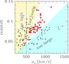 |
Fig. 1 Sample selection of XUCS. The shadedless wedge is the observational optimal locus (clusters fit inside the Swift XRT field of view yet are not too far, so they are not too expensive in terms of exposure time). Points are high-quality clusters in the C4 catalog, red points are those that compose the XUCS sample. |
We collected the few X-ray observations present in the XMM-Newton or Chandra archives and observed the remaining clusters with Swift (individual exposure times between 9 and 31 ks), as detailed in Table 1 of Paper I. Swift observations have the advantage of a low X-ray background (Moretti et al. 2009), making it extremely useful for sampling a cluster population that includes low surface brightness clusters (Andreon & Moretti 2011).
Caustic masses within r200, M200, were derived following Diaferio & Geller (1997), Diaferio (1999), and Serra et al. (2011) and then converted into r500 and M500 assuming a Navarro et al. (1997) profile with concentration c = 5. Adopting c = 3 would change mass estimates by a negligible amount; see Paper I. Basically, the caustic technique performs a measurement of the line-of-sight escape velocity and has the advantage of not assuming virial equilibrium, which is assumed instead when estimating velocity-dispersion-based masses. It only uses redshift and position of the galaxies to identify the caustics on the redshift diagram (clustrocentric distance versus line-of-sight velocity), whose amplitude is a measure of the escape velocity of the cluster. The median number of members within the caustics is 116 and the interquartile range is 45. The median mass of the cluster sample is log M500/M⊙ is 14.2 and the interquartile range is 0.4 dex. The average mass error is 0.14 dex.
3. X-ray analysis
We used X-ray data to measure the surface brightness profile and the spectrum, whose normalization is needed to convert the surface brightness profile into an emissivity profile.
Data reduction was described in Paper I. Briefly, we reduced the X-ray data using the standard data reduction procedures (Moretti et al. 2009; XMMSAS2 or CIAO3). Point sources were detected by a wave detection algorithm and we masked pixels contaminated by them when calculating spectral normalization and radial profiles. In our analysis, we used exposure maps to calculate the effective exposure time accounting for dithering, vignetting, CCD defects, gaps, and excised regions.
Since Swift observations are taken with different roll angles and sometimes different pointing centers, the exposure map may show large differences at very large off-axis angles. To avoid regions of too low exposure, we only considered regions where the exposure time was larger than 50% of the central value. Furthermore, we truncated the radial profile when one-third of the circumference was outside the 50% exposure region defined above. As in Paper I, we take the position of the BCG closest to the X-ray peak as cluster center.
The new part of the data analysis is described below.
3.1. Spectral normalization
In this section we derive the cluster spectral normalization η needed to convert the surface brightness profile into an emissivity profile. The normalization weakly depends on T, and therefore we perform a spectral fit leaving T free and we marginalize over T.
To measure the spectral normalization, we extracted photons in [0.3–7] keV band in two regions: 0.15 <r/r500< 0.5 for the source and the annulus with r/r500> 0.7 and within the 50% exposure region for the background. The cluster central emission was excised to avoid the effects of the possible presence of a central cool core, and the outer radius r/r500 = 0.5 was chosen to maximize the signal-to-noise ratio, following previous literature works (e.g., Croston et al. 2008). The X-ray emission at r/r500> 0.7 is usually very low compared to the background. Moreover, by considering a range of radii, our background estimation is minimally contaminated by the cluster flux. Croston et al. (2008) and Sun et al. (2009), with which we share data for three clusters, also used the local background in their analysis.
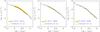 |
Fig. 2 Deprojected electron density profile as derived by us (smooth solid line with shaded 68% bounds) and by Croston et al. (2008; points with error bars). The left-hand panel compares profiles derived from different satellites, whereas the other two panels show analyses sharing (much the same) XMM photons. Profile smoothness and errors depend on assumptions; see text. |
The source spectrum was fit with an absorbed APEC (Smith et al. 2001) plasma model, with the absorbing column fixed at the Galactic value (Dickey & Lockman 1990), the metal abundance fixed at 0.3 relative to solar, and the redshift of the plasma model fixed at optical redshift. The fit accounts for variations in exposure time, excised regions, etc., as mentioned. The spectrum was grouped to contain a minimum of five counts per bin and the source and background data were fitted within the XSPEC spectral package using the modified C-statistic (also called W-statistic in XSPEC). Simulations in Willis et al. (2005) have confirmed that this methodology is reliable (and is now used routinely).
One cluster (CL2081) has data that are too poor to derive a spectrum of quality sufficient to measure a core-excised normalization and therefore was dropped from the sample. The impact of the removal of CL2081 (and of one more cluster dropped in the next section) on our results is discussed in Sect. 4.4.
3.2. Gas density profiles and mass
To measure the gas density profile we assumed a sum of two β models to allow it to deviate from a perfect single β model (e.g., because of the presence of a central cool core). Mathematically, the three-dimensional profile is given by the sum of two β models (with the same slope β)  (1)where ne,i,rc,i,β parameters have the standard meaning. We projected the three-dimensional profile assuming spherical symmetry to obtain the projected gas density. We then converted it into a count-rate profile using the normalization η derived above, and we fit it to unbinned X-ray data to derive best fit parameters and uncertainties. We explored the parameter space by Marcov chain Monte Carlo. We preferred projecting the model instead of de-projecting the data because the latter are noisy and because of the well-known advantages of projection over deprojection (e.g., Pizzolato et al. 2003; Olamaie et al. 2015). Our method builds upon Mohr et al. (1999) and Ettori et al. (2004) and improves upon these works by removing simplifying assumptions (e.g., absence of holes and gaps in the spectral extraction region, a single beta model, binning, Gaussian errors, etc.). Mathematical details are given in Appendix A.
In practice, we extracted the distance from the cluster center r of individual photons in the [0.5–2] keV band, and we fit the projected radial profile without any radial binning (for the latter see Andreon et al. 2008, 2011, 2016, CIAO-Sherpa, and current approaches, such as BayesX; Olamaie et al. 2015; Mantz et al. 2016a). Our fit accounts for vignetting, excised regions, background level, variation in exposure time, and Poisson fluctuations using the likelihood function in Andreon et al. (2008).
The deprojected core-excised gas masses, Mgas,500,ce = Mgas(0.15 <r/r500< 1) are listed in Table 1. The smallest 0.15r500 radius is 49 arcsec, which is much larger than the worse PSF of the instruments used (≲8 arcsec), so that the contribution of any cool-core flux spilled out of the excised region is negligible. Errors are derived by marginalizing over all model (spatial and spectral) parameters.
Although our radial profile model is very flexible (four degree of freedom) in describing the surface brightness profile of clusters, it assumes a unimodal X-ray emission and, therefore, cannot deal with the bimodal CL1022 cluster (Paper I), which we dropped from the sample.
3.3. Gas mass computation checks
We extensively tested our gas masses against our derivations from different X-ray data and by other authors using the same or different X-ray data; we found good agreement, as detailed below. Several of the works we used in the comparison have made different assumptions on temperature profile, have adopted a different annulus to compute the brightness-density conversion, have performed a non-parametric deprojection, have used a different band for computing the brightness profile, or have binned the data. The agreement found indicates that differences in assumptions lead to minor differences to the final result. In particular,
- 1)
Three clusters were observed with Swift and Chandra/XMM.Gas masses derived by different X-ray data differ by less than1σ.
- 2)
Wang et al. (in prep.) kindly recomputed the gas mass of CL3046 using, as we did, Chandra data from the archive, modifying their pipeline to adopt the same r500 and the same annulus we used to convert surface brightness to gas density. The final numbers are identical to ours.
- 3)
The agreement with the unmodified pipeline of Wang et al. (in prep.) for the three clusters in common is better than 0.03 dex for gas masses within their r500. We reproduced the Croston et al. (2008) XMM-Newton results for CL1047 and CL1052 (at their r500) to better than 0.1 dex, using the same XMM data or independent Swift data (CL1047 only). Sun et al. (2009) computed the gas mass fraction within r2500 of Abell 1238 and we agree (at their r2500) at better than 0.1 dex (however, we must point out that we pushed our analysis beyond its limits, at the cluster center, excised in our analysis in Sect. 4).
- 4)
We also compared (Fig. 2) the deprojected electron density profiles of two clusters, CL1047 and CL1052, derived by Croston et al. (2008, points with error bars) and by us (solid curve with 68% errors shaded). We compared the same XMM-Newton data (central and right panel) or data from different telescopes (left panel). The profiles closely match in all cases. The radial profiles show different degrees of smoothness and errors, the amount of which is regulated by the prior, namely the regularization kernel adopted in Croston et al. (2008) and by the assumption of a sum of beta models in our work. Therefore, smoothness and errors can be different for the same analyzed data.
Core-excised gas masses.
3.4. The effect of assuming a β value
Several works (Vikhlinin et al. 2006; Sun et al. 2009; Eckert et al. 2012; Morandi et al. 2015) agreed on a steepening of the gas mass profile close to r500, although the precise location and amplitude of the steepening differ across studies: close to r500, Vikhlinin et al. (2006) found an effective β = 0.78 and Morandi et al. (2015) found β = 0.67 (also adopted in our analysis), whereas Eckert et al. (2012) reported a value in between. To quantify the impact of the β assumed to derive gas masses, we recomputed them adopting the extreme value β = 0.78. These are smaller by 0.03 dex with a scatter of 0.01 dex, both of which are negligible compared to other sources of errors. Gas masses depend little on the assumed slope because the density profile is constrained by the data and a change in slope is compensated by the change of the other four free parameters describing the shape of the profile.
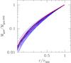 |
Fig. 3 Integrated gas mass profiles scaled to the core-excised gas mass within r500. The gas mass integration starts at 0.15r500. The two clusters with widely different X-ray brightnesses, yet similarities in mass-related properties of Paper I, are plotted in red. |
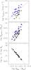 |
Fig. 4 Core-excised [0.5–2] keV luminosity (upper panel), core-excised gas mass (central panel), or a combination of them (bottom panel) vs. caustic mass. The red lines indicate the mean fit from this work (bottom panel) or (top panel) that derived using Eq. (4) from the gas mass slope in Andreon (2010). The squares in the central panel show the expected gas mass derived from LX values in the top panel. These are not plotted for the two open points in the top panel, which are clusters without gas mass estimates. Points indicated in blue are above average in LX | M also turn out to be above average in Mgas | M. Clusters with measurements coming from two X-ray telescopes are shown twice, but the two points may be almost perfectly overlapping in one of the panels (for example, the brightest cluster in the top panel) and therefore do not show up as such. |
4. Results
In Sect. 4.1 we use our X-ray unbiased sample and extend the evidence that gas density profiles are similar across clusters to the whole class of galaxy clusters, extending previous claim restricted to subpopulations of clusters. We use this result to show that this similarity induces a tight covariance between gas mass (or gas mass fraction) and X-ray luminosity, clarifying the profound effect of sample selection on the halo gas mass fraction (Sect. 4.2). In Sect. 4.3 we compute the mean gas mass fraction and its scatter, unveiling a more variegate cluster population than seen so far.
4.1. Similarities of integrated gas mass profiles
Clusters may show a large variety of X-ray luminosities at a given mass because of differences in a) the overall gas mass fraction or b) the shape of the radial profile (see, e.g., Arnaud & Evrard 1999). Figure 3 removes normalization differences by showing the integrated gas mass profiles rescaled by r500 (in abscissa) and by Mgas,500,ce (in ordinate). Profiles are similar, although not identical, indicating a strong similarity of cluster gas integrated density profiles. In particular, we discussed in Paper I two clusters, CL2007 and CL3013, that are significantly different in their X-ray properties (factor 16 in X-ray luminosity and surface brightness) even though they have the same mass, velocity dispersion, richness, redshift, X-ray observations of the same depth and are located in directions characterized by the same Galactic absorption. We highlight these clusters in Fig. 3 (red color). Once scaled to the total gas mass their profiles are entirely consistent with all other profiles in the figure.
The similarity of the scaled gas mass profiles was already established for subpopulations of galaxy clusters (e.g., X-ray selected, relaxed, etc., Croston et al. 2008; Pratt et al. 2009; Mantz et al. 2016b); this evidence is shown here, perhaps for the first time, for the whole population of clusters at a given mass. We emphasize that although we fixed the slope β to 2/3, this only sets the slope of the integrated gas mass profile at large radii but the shape of the profile remains flexible because we use four free parameters (two core radii and two normalizations) to describe the shape. We also emphasize that variations on small spatial scales are washed out by our analysis; studying these variations would require a different analysis and data. Furthermore, exceptions certainly exist, for example, the bimodal CL1022 cluster has a different radial profile by definition, since it is characterized by two centers.
The similarity of the profiles integrated over the same radial range generates a tight, almost scatterless relation between core-excised gas masses Mgas,500,ce, core-excised [0.5–2] keV luminosities LX,ce, and halo masses M500, shown in the bottom panel of Fig. 4,  (2)where the quoted numbers are the median and semi-interquartile range measured on our sample4. This relation differs from the well-know trend between X-ray luminosity and gas mass, where massive clusters tend to be bright and rich of gas compared to their lower mass counterparts. Here, the trend is not driven by mass, the covariance is at a fixed mass; a cluster that is richer in gas by Δ than the average at a given mass (Fig. 4, middle panel) is brighter by 2Δ in LX than the average at a given mass (Fig. 4, top panel).
A relation (with unknown scatter) between gas mass and X-ray luminosity at a fixed mass is expected at least since the work of Arnaud & Evrard (1999): the X-ray luminosity can be written as  , or equivalently
  , which is Eq. (2), with a proportionality constant that depends on the cluster structure (=⟨ ρ2 ⟩ / ⟨ ρ ⟩ 2) and, weakly, on temperature. Since Eq. (2) has a small scatter, we should also see almost the same small scatter for samples that are not representative of the whole cluster population at a given mass (X-ray selected, selected to be relaxed, or just a collection of clusters without any selection function). In fact, by re-analyzing values published in literature we found small scatters (0.03 to 0.04 dex) for a) REXCESS (Pratt et al. 2009; Croston et al. 2008), see also Pratt et al. (2009) analysis; b) the brightest cluster sample of Mantz et al. (2010); and c) clusters in Maughan et al. (2008, see Andreon et al. 2016, for the scatter computation). While the scatter in these samples is small and comparable to what we found, the value derived for XUCS refers to the broader population of all clusters at a given mass. In these works, gas masses and halo masses have been derived in different ways under different assumptions and, therefore, the small scatter we found is not due to a hypothetical (and still unidentified) problem in our data or analysis but is instead the genuine property of clusters.
The low scatter Eq. (2) implies that gas mass can be accurately predicted from the core-excised luminosity and mass, which is listed in Eq. (2) and enters in the determination of r500, as shown in the central panel of Fig. 4 for the XUCS. As obvious from the low scatter of Eq. (2), the gas mass predicted from LX,ce (open squares) is almost coincident with the measured gas mass (solid dots).
The low scatter of Eq. (2) has two additional implications. First, the residuals in LX | M must be tightly correlated with the residuals in Mgas | M to keep the scatter of Eq. (2) low. In particular, the scatter in LX | M should be almost exactly twice the scatter in Mgas | M (exactly so if Eq. (2) were scatterless). The covariance matrix of log LX−log Mgas is therefore 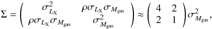 (3)where the second equality is because σMgas ~ 2σLX and because the two scatters are almost perfectly correlated to keep the scatter of Eq. (2) low, i.e., ρ is close to 1. The numerical value of σMgas is derived Sect. 4.3.
Second, the slopes of the relations between X-ray luminosity and gas mass with halo mass, βLX and βMgas, are related by  (4)because a different relation would induce a scatter in Eq. (2). This relation requires, however, confirmation by a sample displaying a larger mass range than probed by XUCS.
Coefficients of covariance matrix and slopes in Mantz et al. (2016b) are consistent with Eqs. (3) and (4), although their analysis is based on a part of the cluster population only (the subsample of relaxed clusters) and ignores the necessary accounting of the effect of sample selection on these quantities. We note that ρ = 0 assumption in Mantz et al. (2016a) disagree with our results.
4.2. Bias of the X-ray selection on halo gas mass fraction
The effect of the selection function on the halo gas mass fraction is considered unclear in previous works (Sun et al. 2012; Laudry et al. 2013; Eckert et al. 2016), assumed to be absent in some scaling relations and cosmological analyses (e.g., Mantz et al. 2010, 2016a5), or was claimed to be important (e.g., Mantz et al. 2016b, unfortunately without accounting for it).
Equation (3) mathematically quantifies that the selection function has direct consequences on the halo gas mass fraction; samples where LX-bright clusters are over-represented are also overly rich in gas-rich clusters. This is illustrated in Fig. 4, where clusters have been color-coded according to their LX | M. Clusters above average in LX | M (top panel) are also above average in their relative gas content for their mass (central panel) and display a smaller scatter than the whole population. This is a consequence of the similarity of gas profiles (Fig. 3), or, equivalently, of the existence of a tight covariance (i.e., ρ = 1) between LX and Mgas. Therefore, accounting for the X-ray selection is essential to derive an unbiased halo gas mass fraction and scatter. If only the blue points are selected and the effects of the selection function are ignored, the mean relation derived would have a higher intercept and a significantly smaller scatter than the whole sample. Therefore, not accounting for the selection on the halo gas mass fraction leads to higher average gas masses and a smaller scatter than the whole population. It is also evident that recovering the red line in the bottom panel, and the full width of the vertical distribution at a given mass using only the blue points would be hard because it would require reconstructing the full range and the correct mean from just the tail of the distribution, while relying heavily on strong assumptions of the properties of the unobserved part of the population.
Therefore, an X-ray selection that is not properly accounted for can have profound implication on the resulting average gas fraction. Moreover, we can also dismiss the qualitative argument that the X-ray selection is negligible because most of the gas mass comes from faint X-ray regions and these are not triggering the X-ray detection. It can be easily proven that all radii outside the core carry similar contributions to the gas mass. Moreover, since the shape of the normalized radial profiles are similar, the gas mass is equally constrained by the X-ray brightness at any radius, not only by those where the X-ray emission is faint.
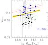 |
Fig. 5 Core-excised gas mass fraction fgas,ce vs. halo mass M500 of XUCS sample with fits to other samples. The black line with shading (error) represents the Andreon (2010) fit to clusters in Vikhlinin et al. (2006) and Sun et al. (2009), the red line represents the Landry et al. (2012, dashed lines indicate scatter) fit to their sample, and the green line represents the XXL 100 brightest clusters (Eckert et al. 2016, dashed lines indicate uncertainty); see text for details. Blue points are clusters that are brighter in X-ray than the average for their mass. |
Figure 5 illustrates the various results one may obtain with different accounting of the selection function on the halo gas mass fraction. The points are core-excised gas mass fractions of the XUCS clusters. This sample, because it is X-ray unbiased, is not affected by the X-ray selection. The clusters show a large scatter in gas mass fraction at a given mass that we quantify in the next section. If only clusters above average in LX | M were available (blue points), the scatter would be biased down and the mean gas mass biased high. In the same figure we plot best fits and error regions obtained by different authors from samples with different selection criteria, but similar mass range. Landry et al. (2013) obtained the best fit at the top of the diagram by studying the most luminous clusters and neglecting the selection function. The representative XUCS sample, which has systematically lower gas mass fractions, confirms the selection bias of the Landry et al. (2013) sample; this possibility is also mentioned, along with others, by the authors. The bottom (green) solid lines in Fig. 5 show the fit to the 100 brightest clusters in the XXL survey (Eckert et al. 2016). Their mean relation is significantly lower, and it appears to be even below the average of our X-ray unbiased sample, which is surprising because the X-ray selection of their sample should favor clusters with large gas mass fractions. This may happen if their weak-lensing cluster masses are overestimated; this possibility is also mentioned, along with others, by the authors. Finally, we also plot the fit derived by Andreon (2010) for the sample in Vikhlinin et al. (2006) and Sun et al. (2009). This sample is formed by relaxed cluster but, apart from that, has an unknown selection function. As quantitatively discussed in next section, our sample (with available selection function) returns a mean gas mass in close agreement with theirs. The fits on samples by Landry et al. (2013), Eckert et al. (2016), Vikhlinin et al. (2006), and Sun et al. (2009) are based on total gas masses, while we plot core-excised gas masses for XUCS. However, this mismatch does not impact our results because of the negligible differences between them for our sample. In fact, including the central emission under the assumption of a constant temperature (which overestimates the gas mass, because excess emission is more likely due to a decrease in temperature rather than higher gas density) would result in gas masses that are higher by ~0.012 dex, with a small scatter of 0.003 dex (semi-interquartile range).
To summarize, the sample selection has the same effect on gas mass than on X-ray luminosity. Clusters for which it is easier to collect large numbers of photons have on average larger-than-average gas masses; if not accounted for, gas mass is biased high and the scatter biased low. The amplitude of the bias is hard to infer from an X-ray selected sample because the width of the LX | M or Mgas | M distribution needs to be either reconstructed from its tail or relies heavily on assumptions and expectations about the behavior of the unobserved population. A similar situations occurs for studied quantities showing a covariance with the quantity used for selecting the sample, such as X-ray luminosity or the strength of the SZ signal when studying the scaling with gas mass. If the sample is X-ray unbiased, i.e., clusters that are brighter-than-average and fainter-than-average for their mass enter with the same probability, the sample selection does not affect the derivation of the halo gas mass fraction or scatter.
4.3. Gas mass fraction: mean and scatter
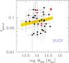 |
Fig. 6 Core-excised gas mass fraction fgas,ce vs. halo mass M500 of XUCS sample. The solid line indicates the mean relations, the shading indicates its 68% uncertainty, whereas the dashed lines indicate the mean relation ± 1σintr. Close pairs of red points (with identical masses) indicate measurements from different X-ray telescopes. |
In this section we fit the relation between gas mass fraction and mass (points in Figs. 5 and 6), allowing intrinsic scatter in fgas | M. We use a linear model with intrinsic scatter σintr that also allows for measurement errors (Dellaportas & Stephens, 1995), which were already used in Andreon (2010; where we also distributed the fitting code) to fit values for clusters in Vikhlinin et al. (2006) and Sun et al. (2009). We fit the data in the gas mass versus halo mass plane, where errors are less correlated (see Andreon 2010). For intrinsic scatter, and log of gas mass fraction at log M/M⊙ = 14, log fgas,14 = log Mgas−14, we assume a uniform and wide range of values that certainly includes the true value. Since we cannot properly determine the slope of the relation in the limited range covered by XUCS clusters, we adopt as prior the posterior derived in Andreon (2010) for the sample in Vikhlinin et al. (2006) and Sun et al. (2009), 0.15 ± 0.03. As shown in Sect. 4.4, the assumption of the slope value does not change the results because the clusters studied have similar masses. The parameter space is sampled by Gibbs sampling using JAGS (see Andreon 2011). For the three clusters for which multiple estimates for gas mass fraction are available, which are derived from different telescopes, the fit only uses those with smaller errors. Our errors on log Mobs incorporate both statistical error and a 20% intrinsic scatter between caustic masses and true masses.
We found  (5)with σintr = 0.17 ± 0.04, signaling that the slope posterior is largely determined by the slope prior.
The results of the fit are plotted in Fig. 6, including the mean relation (solid line), its 68% uncertainty (shading), and the mean relation ± 1σintr.
There is good agreement between the mean scaling derived for the X-ray unbiased sample and for clusters in Vikhlinin et al. (2006) and Sun et al. (2009) samples derived in Andreon (2010), which are reproduced on the top of XUCS clusters in Fig. 5 (the same data shown in Fig. 6). The values of log of gas mass fraction at log M/M⊙ = 14 of the two samples differ by −0.05 ± 0.05 dex, suggesting that the average gas mass fraction is similar in the two samples and that the sample in Vikhlinin et al. (2006) and Sun et al. (2009) does not systematically select gas-rich or gas-poor clusters. The consequences that this agreement has on the hydrostatic mass bias is presented in the companion paper (Andreon et al. 2017). There is also agreement on the slopes, but this occurs because the slope is unconstrained by XUCS data and we assumed the posterior derived for the sample in Vikhlinin et al. (2006) and Sun et al. (2009).
The scatter is robustly measured because our sample selection function does not favor gas-rich clusters at a given mass and, in addition, the selection function is easily characterized at a given mass (a constant). Therefore, we do not need to make assumptions about the unseen population as in X-ray selected samples and the intrinsic scatter is, by large, simply the vertical distribution of the data points after proper accounting of the errors. Our estimate of the scatter, 0.17 ± 0.04 dex, indicates that there is a variable, cluster-to-cluster amount of gas within r500. The scatter we found on the gas mass fraction is larger than values derived in literature, which however only refers to subsamples of the whole cluster population, for example relaxed clusters (e.g., Vikhlinin et al. 2006; Sun et al. 2009; Andreon 2010; Mantz et al. 2016b). For example, clusters in Vikhlinin et al. (2006) and Sun et al. (2009) show a gas mass scatter of 0.06 ± 0.01 dex (Andreon 2010). Our X-ray unbiased sample thus unveils a larger variety in intracluster medium content than past samples focused on subsamples. The large scatter in gas mass fraction could be interpreted as a different fraction of gas being expelled beyond the r500, by, for example, a different amount of feedback from AGN heating the IGM to temperatures in the 108–108.5 range (Le Brun et al. 2014). Alternatively, gas mass fraction differences are present ab initio in the volume occupied by the cluster, but there is no evidence for that in simulations.
The pseudo pressure parameter, YX = MgasT, is believed to be a low-scatter mass proxy (Kravtsov et al. 2006). In Kravtsov et al. (2006) simulations YX has a 0.03 dex scatter with mass, even lower than gas mass scatter, 0.06 dex, because gas mass and temperature are anti-covariant in these simulations. Our gas masses display a scatter that is much larger than Kravtsov et al. (2006) simulations, and simulations by other authors (e.g., Stanek et al. 2010) do not show the anti-covariance between T and Mgas that reduces the scatter of YX below the gas mass scatter, as in Kravtsov et al. (2006). Furthermore, more recent simulations (e.g., Le Brun et al. 2014) suggest, in agreement with our data, that YX is affected by the ICM physics. Therefore, the large gas fraction scatter we found, together with the uncertain theoretical covariance between gas mass and temperature, makes YX a questionable low-scatter mass proxy. The large gas fraction scatter we found also similarly badly affect SZ proxies, such as YSZ = MgasTm (Nagai 2006).
As already mentioned, in scaling relations using X-ray selected samples, or cosmological analyses based on them, the width and center of the distribution (at a fixed mass) of the observable used to select the sample cannot be inferred from the observation of just a tail, i.e., the degeneracy between intrinsic scatter and intercept cannot be broken. A way to break the degeneracy, i.e., to derive intercept and scatter, is to have an estimate of the size of the whole population (assuming a cosmology, for example) and a assumption about the shape of the scatter (lognormal, for example). The latter assumption is strong when the whole population (at a given mass) is not entirely seen, but weak when, as in our case, the whole population is observed. Alternatively, one may assume a prior from simulations, such as the Vikhlinin et al. (2009) cosmological analysis. Our measurement of the intrinsic scatter posterior offers a valid alternative to the use of simulation values, which, as mentioned above, also depend on the implemented subgrid physics.
As mentioned in the introduction, in Paper I we found an amazing variety of X-ray luminosities at a given mass. The similarity of the gas mass density profiles (Sect. 4.1) indicates that the observed large variance is not due to the way the gas mass is distributed within r500. Differences in the overall gas mass fraction are mainly responsible for the wide range of core-excised X-ray luminosities observed in our previous work because the predicted (from Eq. (3)) scatter in LX | M is expected to be twice the gas mass scatter, i.e., 0.34 ± 0.08 (versus the measured 0.47 ± 0.07 dex). To summarize, overall gas differences, from cluster to cluster, are the main source of the variance in core-excised luminosities seen in Paper I.
4.4. Sensitivity analysis
In our analysis, we started from a sample that was not selected based on its X-ray properties. However, we later discarded two (out of 34) clusters because of their X-ray properties.
However, we verified that this does not alter the original properties of the sample. In fact, the almost scatter-less relation between gas mass, X-ray luminosity and halo mass (Eq. (2)) may, at most, acquire two outliers; two objects are too few to erase the bias of X-ray selection on the halo gas mass fraction (Sect. 4.1); they cannot remove the scatter in the Mgas−M relation (Sect. 4.3). We further checked that the intercept of Eq. (5) changes by less than 0.01 dex if we reintroduce the two clusters, using a gas mass predicted from LX (Sect. 4.1).
Our analysis assumes that caustic masses have 20% scatter, as supported by numerical simulations and observations (e.g., Serra et al. 2011; Gifford & Miller 2013; Geller et al. 2013; Maughan et al. 2016). In Andreon et al. (2017) we present a more hypothesis-parsimonous analysis where we leave the scatter free to vary and we marginalize over it. This more rigorous approach confirms the present result of a large gas fraction scatter and therefore a high variable, cluster-to-cluster, amount of gas within r500.
Finally, our analysis of the mean gas mass fraction and scatter assumed as slope prior the posterior of Andreon (2010) based on Vikhlinin et al. (2006) and Sun et al. (2009) clusters. If we instead take a uniform prior on the angle to allow different slopes, we find an identical intrinsic scatter, a very similar intercept −1.17 ± 0.05, as well joint posterior distributions of gas mass fraction and intrinsic scatter close to those derived in our standard analysis. This shows the robustness of our conclusions on assumptions about the slope.
5. Conclusions
We used a cluster sample formed by 34 clusters observed in X-ray in Paper I with caustic masses and whose selection is, at a given cluster mass, independent of the intracluster medium content. We derived gas masses by projecting a flexible radial profile and fitting its projection to the unbinned X-ray data and propagating all modeled sources of uncertainties (e.g., spectral normalization, variation in exposure time including those originated by vignetting or excised regions) with their non-Gaussian behavior (when relevant) into the gas mass estimate using Bayesian methods.
We found that integrated gas density profiles (i.e., the profile shapes) are quite similar, although not identical, extending results based on samples that do not explor the full range of the cluster population at a given mass (e.g., relaxed-only, or X-ray selected, clusters). The overall gas mass fraction is, instead, quite different from cluster to cluster, because the scatter is 0.17 ± 0.04 dex. The scatter we found is larger than found in published samples not exploring the full range of the cluster population at a given mass and indicates a quite variable amount of feedback from cluster to cluster. Our X-ray unbiased cluster sample thus unveiled a part of the cluster population that is underrepresented, when not missed altogether, in X-ray selected samples.
The similarity of the integrated gas density profiles implies a tight relation between core-excised X-ray luminosity, gas mass, and halo mass (Eq. (2)). This implies a) a specific form for the log LX,celog Mgas,500,ce covariance matrix in which the scatter in gas mass is twice the scatter in X-ray luminosity and the correlation coefficient ρ = 1; b) that the slopes of X-ray luminosity and gas mass with halo mass, βLX and βMgas, are related by a simple expression (Eq. (4)); and c) that the effect of the selection function on the halo gas mass fraction is the very same as for X-ray luminosity, i.e., gas-rich clusters are preferentially included in X-ray selected samples.
Finally, the overall gas mass fraction scatter is the main cause of the large variety of core-excised X-ray luminosities observed in our previous work, rather than the way in which the gas mass is distributed within r500.
The radius rΔ is the radius within which the enclosed average mass density is Δ times the critical density at the cluster redshift.
X-ray luminosity is projected, while gas mass is deprojected.
Mantz et al. (2016a) account for the effects of the X-ray selection function on X-ray luminosity but not on gas mass.
For numerical reasons and to improve chain mixing is preferable to reparametrize the model using 60 and 5 arcsec as pivot radii: Σ(b) = Σ0(60)(1 + (60 /rc,0)2)3β−0.5(1 + (b/rc,0)2)− 3β + 0.5 + Σ1(5)(1 + (5 /rc,1)2)3β−0.5(1 + (b/rc,1)2)− 3β + 0.5 + Σbkg. Inside the MCMC sampler and for numerical computation we use this expression.
Acknowledgments
S.A. dedicates this work to the memory of his father Duilio. We thank Adam Mantz for discussion on his papers.
References
- Abazajian, K., Adelman-McCarthy, J. K., Agüeros, M. A., et al. 2004, AJ, 128, 502 [NASA ADS] [CrossRef] [Google Scholar]
- Andreon, S. 2010, MNRAS, 407, 263 [NASA ADS] [CrossRef] [Google Scholar]
- Andreon, S., & Hurn, M. A. 2010, MNRAS, 404, 1922 [NASA ADS] [Google Scholar]
- Andreon, S., & Hurn, M. 2013, Statistical Analysis and Data Mining, 9, 15 [Google Scholar]
- Andreon, S., & Moretti, A. 2011, A&A, 536, A37 [NASA ADS] [CrossRef] [EDP Sciences] [Google Scholar]
- Andreon, S., De Propris, R., Puddu, E., Giordano, L., & Quintana, H. 2008, MNRAS, 383, 102 [NASA ADS] [CrossRef] [Google Scholar]
- Andreon, S., Maughan, B., Trinchieri, G., & Kurk, J. 2009, A&A, 507, 147 [NASA ADS] [CrossRef] [EDP Sciences] [Google Scholar]
- Andreon, S., Trinchieri, G., & Pizzolato, F. 2011, MNRAS, 412, 2391 [NASA ADS] [CrossRef] [Google Scholar]
- Andreon, S., Serra, A. L., Moretti, A., & Trinchieri, G. 2016, A&A, 585, A147 (Paper I) [NASA ADS] [CrossRef] [EDP Sciences] [Google Scholar]
- Andreon, Trinchieri, G., Moretti, A., & Wang, J., 2017, A&A, 606, A25 [NASA ADS] [CrossRef] [EDP Sciences] [Google Scholar]
- Arnaud, M., & Evrard, A. E. 1999, MNRAS, 305, 631 [NASA ADS] [CrossRef] [Google Scholar]
- Becker, M. R., & Kravtsov, A. V. 2011, ApJ, 740, 25 [NASA ADS] [CrossRef] [Google Scholar]
- Cowie, L. L., Henriksen, M., & Mushotzky, R. 1987, ApJ, 317, 593 [NASA ADS] [CrossRef] [Google Scholar]
- Croston, J. H., Pratt, G. W., Böhringer, H., et al. 2008, A&A, 487, 431 [NASA ADS] [CrossRef] [EDP Sciences] [Google Scholar]
- Dellaportas, P., & Stephens, D. 1995, Biometrics, 51, 1085 [CrossRef] [Google Scholar]
- Diaferio, A. 1999, MNRAS, 309, 610 [NASA ADS] [CrossRef] [Google Scholar]
- Diaferio, A., & Geller, M. J. 1997, ApJ, 481, 633 [NASA ADS] [CrossRef] [Google Scholar]
- Dickey, J. M., & Lockman, F. J. 1990, ARA&A, 28, 215 [NASA ADS] [CrossRef] [MathSciNet] [Google Scholar]
- Eckert, D., Vazza, F., Ettori, S., et al. 2012, A&A, 541, A57 [NASA ADS] [CrossRef] [EDP Sciences] [Google Scholar]
- Eckert, D., Ettori, S., Coupon, J., et al. 2016, A&A, 592, A12 [NASA ADS] [CrossRef] [EDP Sciences] [Google Scholar]
- Ettori, S. 2015, MNRAS, 446, 2629 [NASA ADS] [CrossRef] [Google Scholar]
- Ettori, S., Tozzi, P., Borgani, S., & Rosati, P. 2004, A&A, 417, 13 [NASA ADS] [CrossRef] [EDP Sciences] [Google Scholar]
- Geller, M. J., Diaferio, A., Rines, K. J., & Serra, A. L. 2013, ApJ, 764, 58 [NASA ADS] [CrossRef] [Google Scholar]
- Gifford, D., & Miller, C. J. 2013a, ApJ, 768, L32 [NASA ADS] [CrossRef] [Google Scholar]
- Giles, P. A., Maughan, B. J., Dahle, H., et al. 2017, MNRAS, 465, 858 [NASA ADS] [CrossRef] [Google Scholar]
- Hudson, D. S., Mittal, R., Reiprich, T. H., et al. 2010, A&A, 513, A37 [NASA ADS] [CrossRef] [EDP Sciences] [Google Scholar]
- Kravtsov, A. V., Vikhlinin, A., & Nagai, D. 2006, ApJ, 650, 128 [NASA ADS] [CrossRef] [Google Scholar]
- Landry, D., Bonamente, M., Giles, P., et al. 2013, MNRAS, 433, 2790 [NASA ADS] [CrossRef] [Google Scholar]
- Mantz, A., Allen, S. W., Ebeling, H., Rapetti, D., & Drlica-Wagner, A. 2010, MNRAS, 406, 1773 [NASA ADS] [Google Scholar]
- Mantz, A. B., Allen, S. W., Morris, R. G., et al. 2016a, MNRAS, 463, 3582 [NASA ADS] [CrossRef] [Google Scholar]
- Mantz, A. B., Allen, S. W., Morris, R. G., & Schmidt, R. W. 2016b, MNRAS, 456, 4020 [NASA ADS] [CrossRef] [Google Scholar]
- Maughan, B. J., Jones, C., Forman, W., & Van Speybroeck, L. 2008, ApJS, 174, 117 [NASA ADS] [CrossRef] [Google Scholar]
- Maughan, B. J., Giles, P. A., Rines, K. J., et al. 2016, MNRAS, 461, 4182 [NASA ADS] [CrossRef] [Google Scholar]
- Meneghetti, M., Rasia, E., Merten, J., et al. 2010, A&A, 514, A93 [NASA ADS] [CrossRef] [EDP Sciences] [Google Scholar]
- Miller, C. J., Krughoff, K. S., Batuski, D. J., & Hill, J. M. 2002, AJ, 124, 1918 [NASA ADS] [CrossRef] [Google Scholar]
- Miller, C. J., Nichol, R. C., Reichart, D., et al. 2005, AJ, 130, 968 [Google Scholar]
- Mohr, J. J., Mathiesen, B., & Evrard, A. E. 1999, ApJ, 517, 627 [NASA ADS] [CrossRef] [Google Scholar]
- Morandi, A., Sun, M., Forman, W., & Jones, C. 2015, MNRAS, 450, 2261 [CrossRef] [Google Scholar]
- Moretti, A., Pagani, C., Cusumano, G., et al. 2009, A&A, 493, 501 [NASA ADS] [CrossRef] [EDP Sciences] [Google Scholar]
- Navarro, J. F., Frenk, C. S., & White, S. D. M. 1997, ApJ, 490, 493 [NASA ADS] [CrossRef] [Google Scholar]
- Nagai, D. 2006, ApJ, 650, 538 [NASA ADS] [CrossRef] [Google Scholar]
- Nagai, D., Kravtsov, A. V., & Vikhlinin, A. 2007, ApJ, 668, 1 [NASA ADS] [CrossRef] [Google Scholar]
- Olamaie, M., Feroz, F., Grainge, K. J. B., et al. 2015, MNRAS, 446, 1799 [NASA ADS] [CrossRef] [Google Scholar]
- Pacaud, F., Pierre, M., Adami, C., et al. 2007, MNRAS, 382, 1289 [NASA ADS] [CrossRef] [Google Scholar]
- Planck Collaboration IX. 2011, A&A, 536, A9 [NASA ADS] [CrossRef] [EDP Sciences] [Google Scholar]
- Pizzolato, F., Molendi, S., Ghizzardi, S., & De Grandi, S. 2003, ApJ, 592, 62 [NASA ADS] [CrossRef] [Google Scholar]
- Pratt, G. W., Croston, J. H., Arnaud, M., & Bohringer, H. 2009, A&A, 498, 361 [NASA ADS] [CrossRef] [EDP Sciences] [Google Scholar]
- Serra, A. L., Diaferio, A., Murante, G., & Borgani, S. 2011, MNRAS, 412, 800 [NASA ADS] [Google Scholar]
- Smith, R. K., Brickhouse, N. S., Liedahl, D. A., & Raymond, J. C. 2001, ApJ, 556, L91 [NASA ADS] [CrossRef] [Google Scholar]
- Stanek, R., Rasia, E., Evrard, A. E., Pearce, F., & Gazzola, L. 2010, ApJ, 715, 1508 [NASA ADS] [CrossRef] [Google Scholar]
- Sun, M. 2012, New J. Phys., 14, 045004 [NASA ADS] [CrossRef] [Google Scholar]
- Sun, M., Voit, G. M., Donahue, M., et al. 2009, ApJ, 693, 1142 [NASA ADS] [CrossRef] [Google Scholar]
- Vikhlinin, A., Kravtsov, A., Forman, W., et al. 2006, ApJ, 640, 691 [NASA ADS] [CrossRef] [Google Scholar]
- Vikhlinin, A., Burenin, R. A., Ebeling, H., et al. 2009, ApJ, 692, 1033 [NASA ADS] [CrossRef] [Google Scholar]
- Willis, J. P., Pacaud, F., Valtchanov, I., et al. 2005, MNRAS, 363, 675 [NASA ADS] [CrossRef] [Google Scholar]
Appendix A: Calculating gas densities profiles and masses
Let us consider a three-dimensional profile given by the sum of two β models (with the same slope β)  (A.1)where ne,0,ne,1 are the central densities and rc,0,rc,1 are the core radii.
The projection in two dimensions is analytically known  (A.2)where the last term accounts for the background6.
The relation between the normalizations  and Σi is given by
  (A.3)(Cowie et al. 1987; Hudson et al. 2010; Ecker et al. 2016), where the second equality accounts for the fact that we do not measure projected densities Σi’s, but brightnesses ci = Σi/k whereas the third equality comes from defining
  . The symbol Γ is the usual Gamma function. Therefore, a fit to the radial profile returns the core radii rc,i, β values, and coefficients, the latter up to a constant k′ that we now determine. We derive it from the normalization of the spectral fit η (returned by XSPEC, as described in Sect. 3.1) defined by
  (A.4)where dA is the cluster angular distance. In fact, by definition
  (A.5)where we assume np = 0.82ne and the integral is over the “cylinder” having as base the spectral extraction region Ω and extends all along the line of sight.
Equating the right-hand sides of Eqs. (A.4) and (A.5), inserting Eq. (A.1) into the latter, and substituting with the right-hand side of Eq. (A.3) gives ![Mathematical equation: \appendix \setcounter{section}{1} \begin{eqnarray} k' &= \dfrac{4 \pi d^2_{\rm A} (1+z)^2 \eta 10^{14}}{0.82 \int_\Omega \left[\dfrac{c_{0}}{r_{\rm c,0}} (1\!+\!(r/r_{\rm c,0})^2)^{-3\beta}\! +\! \dfrac{c_{1}}{r_{\rm c,1}} (1\!+\!(r/r_{\rm c,1})^2)^{-3\beta} \right] {\rm d}V} , \nonumber\\ &= \dfrac{4 \pi d^2_{\rm A} (1+z)^2 \eta 10^{14}}{0.82 c_\eta} , \end{eqnarray}](/articles/aa/full_html/2017/10/aa30722-17/aa30722-17-eq116.png) (A.6)where cη = ∫Ω [ ... ] dV is the net counts in the imaging extraction band in the spectral extraction region used to compute η, which is known.
(A.6)where cη = ∫Ω [ ... ] dV is the net counts in the imaging extraction band in the spectral extraction region used to compute η, which is known.
Since there are no left unknowns, deprojected gas masses can now be straightforwardly computed from  (A.7)where μemp is the mean atomic mass, starting the integration from 0.15r500 when core-excised masses are needed.
The parameter β is fixed at 2/3 because our data cannot constrain all model parameters for every cluster when using the sum of two beta models to describe the profile. Section 3.4 explores the effect of this assumption. For the other parameters, we took weak priors, and, in particular, we took a uniform prior for Σi’s and Σbkg, constrained to be positive (to avoid unphysical values), and a Gaussian prior on the core radius rc,1 with the center equal to r500/ 5 (suggested by Ettori et al. 2015), with a 30% sigma (i.e., rc,1 ∈ (0,r500) with 99 % probability). Finally, we ask that the second component (modeling the cool core) is much smaller than the cluster itself (i.e., rc,0 < rc,1/ 5). A posteriori, all (posterior mean) rc,0 and rc,1 are well within these ranges. Chandra data also require us to excise the inner 3–5 arcsec region because of the unmodeled BCG emission.
All Tables
All Figures
|
Fig. 1 Sample selection of XUCS. The shadedless wedge is the observational optimal locus (clusters fit inside the Swift XRT field of view yet are not too far, so they are not too expensive in terms of exposure time). Points are high-quality clusters in the C4 catalog, red points are those that compose the XUCS sample. |
| In the text | |
|
Fig. 2 Deprojected electron density profile as derived by us (smooth solid line with shaded 68% bounds) and by Croston et al. (2008; points with error bars). The left-hand panel compares profiles derived from different satellites, whereas the other two panels show analyses sharing (much the same) XMM photons. Profile smoothness and errors depend on assumptions; see text. |
| In the text | |
|
Fig. 3 Integrated gas mass profiles scaled to the core-excised gas mass within r500. The gas mass integration starts at 0.15r500. The two clusters with widely different X-ray brightnesses, yet similarities in mass-related properties of Paper I, are plotted in red. |
| In the text | |
|
Fig. 4 Core-excised [0.5–2] keV luminosity (upper panel), core-excised gas mass (central panel), or a combination of them (bottom panel) vs. caustic mass. The red lines indicate the mean fit from this work (bottom panel) or (top panel) that derived using Eq. (4) from the gas mass slope in Andreon (2010). The squares in the central panel show the expected gas mass derived from LX values in the top panel. These are not plotted for the two open points in the top panel, which are clusters without gas mass estimates. Points indicated in blue are above average in LX | M also turn out to be above average in Mgas | M. Clusters with measurements coming from two X-ray telescopes are shown twice, but the two points may be almost perfectly overlapping in one of the panels (for example, the brightest cluster in the top panel) and therefore do not show up as such. |
| In the text | |
|
Fig. 5 Core-excised gas mass fraction fgas,ce vs. halo mass M500 of XUCS sample with fits to other samples. The black line with shading (error) represents the Andreon (2010) fit to clusters in Vikhlinin et al. (2006) and Sun et al. (2009), the red line represents the Landry et al. (2012, dashed lines indicate scatter) fit to their sample, and the green line represents the XXL 100 brightest clusters (Eckert et al. 2016, dashed lines indicate uncertainty); see text for details. Blue points are clusters that are brighter in X-ray than the average for their mass. |
| In the text | |
|
Fig. 6 Core-excised gas mass fraction fgas,ce vs. halo mass M500 of XUCS sample. The solid line indicates the mean relations, the shading indicates its 68% uncertainty, whereas the dashed lines indicate the mean relation ± 1σintr. Close pairs of red points (with identical masses) indicate measurements from different X-ray telescopes. |
| In the text | |
Current usage metrics show cumulative count of Article Views (full-text article views including HTML views, PDF and ePub downloads, according to the available data) and Abstracts Views on Vision4Press platform.
Data correspond to usage on the plateform after 2015. The current usage metrics is available 48-96 hours after online publication and is updated daily on week days.
Initial download of the metrics may take a while.