| Issue |
A&A
Volume 606, October 2017
|
|
|---|---|---|
| Article Number | A23 | |
| Number of page(s) | 27 | |
| Section | Extragalactic astronomy | |
| DOI | https://doi.org/10.1051/0004-6361/201730683 | |
| Published online | 02 October 2017 | |
Primordial environment of supermassive black holes
II. Deep Y- and J-band images around the z ~ 6.3 quasar SDSS J1030+0524
1 INAF–Osservatorio Astronomico di Bologna, via Piero Gobetti 93/3, 40129 Bologna, Italy
e-mail: This email address is being protected from spambots. You need JavaScript enabled to view it.
2 Dipartimento di Fisica e Astronomia, Alma Mater Studiorum, Universitá degli Studi di Bologna, via Piero Gobetti, 93/2, 40129 Bologna, Italy
3 Department of Physics, Yale University, PO Box 208121, New Haven, CT 06520, USA
4 Yale Center for Astronomy & Astrophysics, Physics Department, PO Box 208120, New Haven, CT 06520, USA
5 European Southern Observatory, Alonso de Cordova 3107, Casilla 19, 19001 Santiago, Chile
6 Department of Astronomy and Astrophysics, 525 Davey Lab, The Pennsylvania State University, University Park, PA 16802, USA
7 Institute for Gravitation and the Cosmos, The Pennsylvania state University, University Park, PA 16802, USA
8 Scuola Normale Superiore, Piazza dei Cavalieri 7, 56126 Pisa, Italy
Received: 23 February 2017
Accepted: 6 June 2017
Abstract
Many cosmological studies predict that early supermassive black holes (SMBHs) can only form in the most massive dark matter halos embedded within large-scale structures marked by galaxy overdensities that may extend up to ~10 physical Mpc. This scenario, however, has not been confirmed observationally, as the search for galaxy overdensities around high-z quasars has returned conflicting results. The field around the z = 6.31 quasar SDSSJ1030+0524 (J1030) is unique for multi-band coverage and represents an excellent data legacy for studying the environment around a primordial SMBH. In this paper we present wide-area (~25′ × 25′) Y- and J-band imaging of the J1030 field obtained with the near infrared camera WIRCam at the Canada-France-Hawaii Telescope (CFHT). We built source catalogs in the Y- and J-band, and matched those with our photometric catalog in the r, z, and i bands presented in our previous paper and based on sources with zAB< 25.2 detected using z-band images from the the Large Binocular Cameras (LBC) at the Large Binocular Telescope (LBT) over the same field of view. We used these new infrared data together with H and K photometric measurements from the MUlti-wavelength Survey by Yale-Chile (MUSYC) and with the Spitzer Infrared Array Camera (IRAC) data to refine our selection of Lyman break galaxies (LBGs), extending our selection criteria to galaxies in the range 25.2 <zAB< 25.7. We selected 21 robust high redshift candidates in the J1030 field with photometric redshift z ~ 6 and colors i−z ≥ 1.3. We found a significant asymmetry in the distribution of the high redshift galaxies in J1030, supporting the existence of a coherent large-scale structure around the quasar. We estimated an overdensity of z ~ 6 galaxies in the field of δ = 2.4, which is significant at >4σ. The overdensity value and its significance are higher than those found in our previous paper and we interpret this as evidence of an improved LBG selection.
Key words: galaxies: high-redshift / galaxies: photometry
© ESO, 2017
1. Introduction
Supermassive black holes (SMBHs), found at the center of distant (z> 6) and very luminous (>1047 erg s-1) quasars (QSOs), are among the most challenging astronomical objects ever observed (Mortlock 2016; Wu et al. 2015). The mechanism by which these SMBHs of 109−10M⊙ formed and grew when the universe was only 1 Gyr old is the subject of many theoretical speculations. Recent simulations show that early SMBHs can only form in the most massive dark matter halos, that could eventually evolve into the present-day clusters of galaxies with M> 1014−15M⊙ (Costa et al. 2014). As such, high-z QSOs would be part of early large-scale structures marked by large galaxy overdensities that may extend up to radii of ~10 physical Mpc (pMpc) (e.g., Overzier et al. 2009; Di Matteo et al. 2012; Angulo et al. 2013), corresponding to Δz ± 0.15 in redshift space at z = 6. Furthermore, these regions are expected to evolve at a substantially accelerated pace and may be populated by galaxies that are more massive, dusty, and star-forming than those in average-density fields, reaching star formation rates as high as ≳700 M⊙ yr-1 (Yajima et al. 2015).
Understanding how the largest observed structures formed has fundamental implications for the standard formation model of the Universe. The suggested theoretical scenario is not confirmed, since currently we lack clear observations of the environment in which high-redshift QSOs reside. This research line has produced discrepant results: different authors found number densities of Lyman break galaxies (LBGs) around high-z QSOs that are higher (e.g., Garcia-Vergara et al. 2017 at z ~ 4), lower, or consistent with what is expected in blank fields (Kim et al. 2009). One possible reason for these inconsistent results is that most attempts used small fiel of view (FoV) instruments, like the 3′ × 3′ Advanced Camera for Surveys (ACS) on board the Hubble Space Telescope (HST), or 6′ × 6′ imagers at best (e.g., Stiavelli et al. 2005; Husband et al. 2013; Simpson et al. 2014; Mazzucchelli et al. 2017), equivalent to distances of ~0.5–1 pMpc from the QSO, whereas these structures may extend well beyond. Furthermore, the intense UV radiation and gas outflows released by the quasar (feedback effects) might affect its environment, ionizing and heating the intergalactic medium up to several Mpc away (e.g., Rees 1988; Babul & White 1991). Star formation might be prevented, especially in less massive galaxies, and this could cause the observed deficiency of Lyα emitters (LAEs) around QSOs (Kashikawa et al. 2007; Overzier 2016; Mazzucchelli et al. 2017). Therefore, the presence of an overdensity of galaxies might then be best explored at larger scales. Indeed, measurements performed with the wide-field 33′ × 27′ Suprime-Cam at the Subaru Telescope revealed tentative evidence of an overdensity around two z ~ 6 QSO (Utsumi et al. 2010; Díaz et al. 2014), one of them being in fact SDSS J1030+0524 (Díaz et al. 2014).
With the goal of understanding the environmental properties of distant quasars on wide scales, we started a multi-wavelength campaign in the fields around high-redshift QSOs. In 2012 we obtained deep r, i, z imaging with the Large Binocular Camera (LBC) at the Large Binocular Telescope (LBT) of the fields around four QSO observed in the Sloan Digital Sky Survey (SDSS) in the redshift range z = 5.95−6.41, selected to have MBH> 109 M⊙. We produced photometric catalogs of all the sources detected in z-band. To identify candidate galaxies around the redshift of the quasars, we applied the drop-out technique (e.g., Steidel et al. 1996; Dickinson et al. 2004; Bouwens et al. 2015; Vanzella et al. 2009), looking for the Lyman-α break feature that at z ~ 6 is redshifted between the i- and z-band. The LBC data depth, combined with the large FoV (~25′ × 25′), allowed us to make a selection of i-band dropout galaxies down to zAB = 25.2 (5σ) in a sky area corresponding to ≈8 × 8 pMpc2 at z ~ 6.
After accounting for cosmic variance and photometric errors, we measured an i-band dropout overdensity in all fields, with significance ranging from 1.7 to 3.3σ (3.7σ when combining the four fields, Morselli et al. 2014, in the following M14). This suggests that the dense environment around early QSOs is best traced on large scales.
In this paper we focus on the most overdense of our fields, that is, the one around the z = 6.31 QSO SDSS J1030+0524 (hereafter the J1030 field). We present deep Y- and J-band imaging with the near infrared camera (WIRCam) at the Canada-France-Hawaii Telescope (CFHT) to integrate our photometric source catalog with these two bands. These data are essential to discriminate between high-redshift galaxies and stellar contaminants, by building diagnostic color-color diagrams or computing robust photometric redshift estimation. Deep imaging with the Infrared Array Camera (IRAC) on board Spitzer at 3.6 and 4.5 μm is available for most objects and some targets have been also detected in the MUlti-wavelength Survey by Yale-Chile (MUSYC, Quadri et al. 2007; Blanc et al. 2008). Our team was also granted 500 ks with the X-ray telescope Chandra in 2015 (the observations are ongoing) with the main aim to search for the first detection of “satellite” AGN in this high density environment. All the data we are collecting make this field an excellent legacy for many different investigations. We made the photometric LBT catalogs publicly available at the project website1.
The purpose of this paper is two-fold. First, we present the new Y- and J-band photometric catalog in the J1030 field. We describe the observations (Sect. 2) and how we combine the Y and J photometry with the optical r, i, z multicolor catalog (Sect. 3). Second, we use these data to improve the reliability of our LBG candidates using color plots and building the spectral energy distributions (SEDs) to derive photometric redshifts (Sect. 4). We discuss our results in Sect. 5 and we present our summary and conclusions in Sect. 6. Unless otherwise indicated, magnitudes are given on the AB system, for which, by definition, a constant flux of 3720 Jy represents mag = 0. Throughout the paper we use H0 = 70 km s-1 Mpc-1, Ωm = 0.3, and ΩΛ = 0.7.
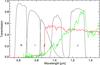 |
Fig. 1 Response filter curves of the WIRCam camera in the Y- and J-bands and for LBT/LBC r, i, and z bands (SDSS-like filters). We show in red a star-forming galaxy template at z = 6.3 with age 0.5 Gyr and Z = 0.02Z⊙ (from Bruzual & Charlot 2003) and in green a template of a T-type dwarf star from the SpeX Prism Spectral Libraries. |
2. Observations and data analysis
2.1. Observations
The observations were performed at the 3.6 m Canada-France-Hawaii Telescope (CFHT) located at Mauna Kea, Hawaii, with the Wide-field InfraRed Camera (WIRCam) on the nights of December 23–24, 2015, under excellent seeing conditions. These data were obtained through the Optical Infrared Coordination Network for Astronomy (OPTICON) access program. The field of view of the camera is ~21′ × 21′ and the pixel scale is 0.306″/pixel, well matching the size and the resolution of our LBC observations of the field. We selected the Y and J broad band filters, centered at 1.020 and 1.253 μm respectively. In Fig. 1 we report the instrumental response functions.
We received pre-processed single images data from CFHT (dark subtracted and flat field corrected), and deeper J and Y images stacked in a mosaic from TERAPIX2. Individual exposures were combined using the software SWarp. Precise astrometric and photometric calibrations, as well as accurate sky subtraction and quality assessment, were performed by the TERAPIX team on the final mosaic. Because of the adopted dithering pattern, the Y- and J-band images cover the entire 25′ × 25′ FoV of the LBT/LBC imaging data. The total magnitudes have been compared to the aperture-corrected magnitudes from the public Two Micron All-Sky Survey (2MASS) point-source catalog to determine the zero point of the image, that is, the magnitude at which the flux is 1 photon/s. The zero-points, based on AB photometric system, are reported in Table 1, along with the total exposure time, the seeing in the final mosaic (computed measuring the Full With Half Maximum (FWHM) of morphological and color selected star candidates), and the Galactic dust absorption correction factor.
Basic data information.
2.2. Photometric catalog in the Y- and J-band
We used the software SExtractor version v2.19.5 (Bertin & Arnouts 1996) to detect objects in the Y- and J-band images. All the input parameters are fixed to the software default values except the photometric zero-points, corrected for Galactic dust extinction, for the aperture correction, and the seeing, adopting the values reported in Table 1 . On the clean regions of the WIRCam images (after masking the noisy edges which are a product of the dithering), we detect 13540 (14770) objects down to YAB ≈ 25 (JAB ≈ 24.5), and the similar number of detected sources in the two bands attests to the good balanced choice of exposure times. Our optical photometric catalog, based on source detection in the z-band image, contains ~2.7 × 10⁴ objects above the 50% completeness limit3 of zAB = 25.2 mag at 5σ (M14). We cross-correlated the LBC photometric catalog with the new Y and J catalogs, finding that about 49% (46%) of the objects detected in the z-band are detected in the Y- (J-) band. Conversely, 94% (91%) of the source detected in the Y- (J-) bands catalogue are detected in the LBC z optical bands.
2.3. Multi-band photometric measurements
We use the IDL routine aper (adapted from the IRAF/DAOPHOT package) to measure the brightness of LBG candidates in the Y- and J-band, assuming a circular aperture of radius 0.8″ (in M14 we chose this aperture size to collect a large fraction of the flux from the object while minimizing the contamination from neighboring sources). Comparing the magnitude measured in the adopted aperture with the total magnitude measured for a sample of stars, we derived the correction factor for the aperture that takes into account the flux lost outside the aperture in unresolved sources due to seeing conditions (see Table 1). In the following we will use the aperture-corrected magnitude for the photometric color measurements, a good proxy for the total magnitude for our faint, unresolved targets. We estimate the background in an annulus between five and ten pixel radius. For the Spitzer/IRAC images we adopt a 3.2 pixel radius (1.9″) and we subtract the background emission. To correct extended source photometry, we apply the functional form for the photometrical correction coefficients for the adopted circular aperture radius4. Flux errors are estimated adding three terms in quadrature: 1) random noise inside the aperture as estimated by the scatter in the sky values; 2) the Poisson statistics of the observed target brightness; 3) the uncertainty of the mean sky brightness.
When the source detection does not reach a signal-to-noise ratio (S/N, defined as the ratio of the measured flux S over the uncertainty N) of at least a factor of two, we estimate an upper limit for the flux at the 2σ confidence level. We repeat this analysis also for the LBT/LBC r- and i-band images to obtain local upper limits (we note that in M14 upper limits averaged across the entire images were considered). We estimate the limiting magnitude at the position of each target by measuring the total flux in 200 circular regions (with the same radius of the extraction region) randomly selected within 50″ from the source. The flux distribution is peaked around zero but it appears skewed to the right, because positive sky pixel values due to undetected sources contaminate the background measurements. Therefore, to provide a robust estimate of the noise level, we evaluate the rms of the flux distribution by mirroring its negative part. We convert this value into a magnitude taking into account the aperture correction and finally we estimate the 2σ upper limits adopted throughout the paper.
3. Selection of LBGs around high-z QSO
Here we enlarge the number and improve the robustness of possible z ≈ 6 galaxy candidates in the J1030 field with respect to M14. The redshift window sampled by the i-band dropout technique is broad (z ~ 5.6–7, adopting a color threshold of i−z > 1.3, e.g., Beckwith et al. 2006), but we note that even objects at redshifts significantly different from that of the central QSO can still be part of its large structure (e.g., Δz = 0.15 at z = 6 is ~10 pMpc, consistent with the large-scale structure size in the Overzier et al. 2009, simulations).
Several contaminants at lower redshift can survive the i−zcolor selection. The most numerous ones are expected to be dwarf stars of M, L, and T types in our Galaxy, whose colors can match those of candidate high-z galaxies. Additionally, dusty star-forming galaxies and obscured AGN at lower redshift can mimic the Lyman break of a true high redshift galaxy. Finally, the Balmer break at 4000 Å (D4000) of a passively evolving galaxy at z ~ 1.1 can be mistaken for the Lyman break (Dunlop 2013; Finkelstein 2016).
Full details on the adopted optical color selection criteria can be found in M14. Briefly, since most of the spectroscopically confirmed galaxies at redshift ~6 show i−z colors greater than 1.3 (e.g., Vanzella et al. 2009), we adopted this threshold value. In M14 we then created a catalog of LBC primary dropouts adopting a stringent criterion (i−z)−σ(i−z)> 1.3 and requiring that these objects are undetected in the r-band at 3σ (rAP > 27.2) and are detected at 5σ in the z-band with zAB < 25.2, our completeness limit. In addition, in order to investigate the presence of interesting high-z outliers to be followed-up spectroscopically among bluer objects (e.g., the few galaxies at z ~ 5.7 with strong Lyα emission among the vast majority of stars and low-z galaxies), we created a catalog of secondary drop-out candidates by relaxing our color criteria [1.1 < (i−z)−σ(i−z) < 1.3]. In fact, these objects were excluded from the estimation of the overdensity levels in M14.
Here we extended our analysis to z ~ 6 LBG candidates at fainter magnitudes. In particular we selected objects undetected in the r band, with 25.2 <zAB < 25.7(5σ), and color i−z ≥ 1.3. At zAB > 25.2 the predicted number density of z ~ 6 LBGs is higher than that of dwarf stars, since the predicted number of dwarf stars declines at brighter magnitudes, while the expected count of high redshift LBGs increases at fainter magnitudes. The selection of high-z LBGs should therefore be less susceptible to star contamination below this magnitude threshold (see Fig. 2 in Bowler et al. 2015). We visually inspected the images of all the candidates and rejected obvious image artifacts or problematic objects close to luminous stars or on the image edges. At the end of the process we selected 18 new LBG candidates which we refer to as faint candidates. In Fig. 2 we present the J1030 field in the J- and Y-band, with overlaid in different colors the primary and secondary candidates of M14 and the new faint candidates. In Table 2 we report the full photometric information for all these samples.
Multi-band photometry for the sample LBG primary, secondary and faint candidates.
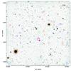 |
Fig. 2 CFHT/WIRCam Y and J two-color-composite image of the 1030 field. The image is ~24′ × 24′ and covers the entire LBT/LBC field of view (FoV). North is up and east is to the left. The central SDSS QSO at z = 6.31 is shown as a magenta circle. The LBG primary and secondary i-band dropouts of M14 are shown as red and green circles, respectively. Blue circles mark the new faint candidates (see text for details). |
3.1. Color-color diagram
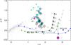 |
Fig. 3 Diagnostic (z−Y) versus (i−z) color-color diagram. Small gray dots are point-like sources in the J1030 field (star locus). Red, green, and cyan are the primary and secondary candidates of M14 and the new faint candidates, respectively. For those objects that are not detected at the 2σ level in i or in Y, we used the 2σ local limiting magnitudes. The limits on their colors are marked with arrows. The black curve shows the expected color track (in steps of Δz = 0.1, starting from 5.5) of a high-z star-forming galaxy with age 0.5 Gyr and Z = 0.02 Z⊙ (from Bruzual & Charlot 2003). The gray curve has been calculated with the same template but with an intrinsic absorption Av equal to one and the green curve adding to the template a Lyα emission line with EW = 100 Å rest frame. The blue curve shows the expected color track of a Type 1 QSO (template from the SWIRE library). Objects that have now been classified as reliable z ~ 6 LBGs (see Table 3 and Sect. 4) are marked with large black open circles. The bigger magenta circle and the diamond symbol represent the colors of the stack of the LBG candidates and stellar contaminants, respectively. The blue point marks the position of the central QSO SDSS J1030+0524 at z = 6.31. |
A widely used technique to separate contaminants from genuine LBGs at z ~ 6 is to use color-color diagrams that involve near-IR magnitudes. In particular, color-color diagrams involving the i-, z-, and Y-bands are effective in isolating candidate LBGs at z> 6 (Bowler et al. 2015; Matsuoka et al. 2016).
In Fig. 3 we show the position of our candidates in the z−Y versus i−z color-color diagram. The small gray dots represent the color of point-like sources, likely stars in the J1030 field, selected to have the Sextractor morphological parameter CLASS_STAR > 0.95 and stellar optical colors. The red, green, and cyan points represents the primary, secondary and faint candidates. Using the Hyperz code (Bolzonella et al. 2000), we derived the expected colors of a typical starburst galaxy and of a quasar at redshifts greater than 5.5, taking into account the Inter Galactic Medium (IGM) absorption and the convolution with the transmission function of the adopted filter. We assumed a template from Bruzual & Charlot (2003) with age 0.5 Gyr and metallicy Z = 0.02Z⊙ for the star-forming galaxy, and a type 1 QSO template from the SWIRE library for the quasar (Polletta et al. 2007). All the 42 candidates are detected in the z band by selection, and show upper limits to the z−Y color if undetected in the Y band and lower limits to the i−z color if undetected in the i band. Nineteen objects, mostly from the faint sample, have limits in both colors.
3.2. Morphological classification of LBGs
To perform a morphological classification, we use the classical aperture corrected magnitude versus the total magnitude diagnostic plot, since the ratio between these two quantities represents a robust index of source concentration. By applying this diagnostic to the band with the highest S/N candidate detection, we classify all the primary and secondary targets as extended or point-like (flag “e” or “p”). We do not attempt to assign a morphological description to the fainter candidates, since the technique is not reliable at the very faint flux level. We use the morphological classification as an exclusion criteria, taking out the stellar templates in the photometric redshift estimate in case of extended source. In fact, while the brown dwarf stars are always unresolved, the Lyman break galaxies could appear as spatially extended in ground based images. For example, Willott et al. (2013) found that about 50% of their sample of galaxies at z ~ 6 are spatially resolved in 0.7 arcsec seeing images.
Colors, morphology, photometric redshift and final classification for our candidates.
3.3. Photo-z estimation of LBGs
In order to obtain photometric redshift measurements, we built the spectral energy distribution (SED) of the LBG candidates, with aperture-matched, multi-band photometry, extending as much as possible the wavelength range considered. So, along with the new Y and J WIRCam observations, we use the optical r, i, z photometric measurements (in blue-ward optical bands we do not have images deep enough to detect sources with expected AB magnitudes fainter than 28, the median global upper limit in the r-band in M14). We searched for H and K photometric measurements in the MUSYC survey, which includes a wide part covering our entire field down to a typical 5σ limit of KAB = 21.7 (Blanc et al. 2008) and a central and deeper region of 10′ × 10′ down to HAB and KAB of 22.9 in both bands (5σ). We found that two primary candidates are detected in the H-band (four in the K-band) and three secondary candidates are detected both in the H- and K-bands. Finally we searched the Spitzer Heritage Archive (SHA) for IRAC images in the 3.6 and 4.5 μm bandpasses (ch1 and ch2, respectively) to extend the photometric SED at longer wavelengths. Two Program IDs (namely 30873 and 10084) cover more than half of the field once combined. Only three primary and one secondary candidates have no Spitzer photometric coverage in the IRAC 3.6 band (three and one in the IRAC 4.5 band). We downloaded the Level 2 images of these two datasets, and we perform photometry of the targets as described in Sect. 2.3.
We used Hyperz to refine our redshift estimates and pinpoint low-z interlopers. The photometric redshifts are based on a χ2 fitting procedure to the observed fluxes (or magnitudes) and photometric errors. The SED is matched to the galaxy templates, convolved with the filter response in each of the input bands, and corrected for the absorption by intervening HI clouds following the Madau (1995) prescription. In the literature, updated versions of the so-called Madau model for the IGM attenuation have been proposed (e.g., Meiksin 2006; Inoue et al. 2014). However, the differences in the predicted colors and in the photometric redshift estimates should be small (about 0.05, see Inoue et al. 2014). We also accounted for possible internal reddening assuming the Calzetti extinction law (Calzetti et al. 2000). If an object is not detected in one band we set its flux to Flim and its 1σ error to Flim/2, where Flim is the flux corresponding to the 2σ limiting magnitude in that band.
Our primary templates are the four templates of Coleman et al. (1980) observed spectra (Ell, Sbc, Scd, Irr) extended into the UV and NIR using the spectral synthesis models of the Galaxy Isochrone Synthesis Spectral Evolution Library (GISSEL98; Bruzual & Charlot 1993). These five templates are linearly interpolated to produce a total of 62 templates as described in Ilbert et al. (2006). We add an observed starburst SED from Kinney et al. (1996) and six additional templates generated using Bruzual & Charlot (2003, hereafter BC03) models with starburst (SB) ages of 0.05, 0.15, and 0.50 Gyr, and metallicity 0.02 and 0.2 solar. These templates are commonly used to estimate photometric redshifts (Brodwin et al. 2006; Ilbert et al. 2006). Finally, to account for stellar contamination, we add the 21 models of dwarf stars of ML and T type from the SpeX Prism Spectral Libraries5 whose colors can match those of our candidate galaxies. We extend the stellar templates from 2.5 to 4.5 μm assuming a simple power-law Fν ~ να with α = −4. We fit each photometric SED using the two sets of templates separately, considering a redshift range between 0 and 0.01 and between 0 and 7 for the stellar and galaxy solution, respectively, and we discriminate between the two solutions according to the χ2 value. We note that in many cases we obtained very low values for the reduced χ2 because of the many upper limits in the SEDs.
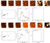 |
Fig. 4 Example of our classification strategy based on morphology, colors, and photometric redshift for two z ~ 6 LBG candidates in the J1030 field, that we respectively classified as likely star (upper panel) and highz objects (lower panel). Upper panel (same for the lower panel): a) postage stamps (7′′ on a side) in the r, i, z, Y, J, IRAC/ch1, IRAC/ch2 filters. We note that the apparent mismatch of the point sources in the IRAC images is due to the lack of Spitzer data for some targets. b) Photometric colors diagnostic plot. The small black dots are stars in the field and the dashed line represents an extrapolation of the stellar locus based on the colors of known M, L, and T-type dwarfs. The red point represents the color of the LBG candidate. c) SED fitting and photometric redshift determination for the same candidate. Blue squares represent AB magnitudes in r, i, z, Y, J, and Spitzer/IRAC ch1 and ch2 bands with 1σ-error. The best fit is shown with a red line for galaxy and with a green line for stellar case solutions. We report the χ2 for the two template solutions. d) Corresponding probability distribution of the best fit as a function of redshift. We present these summary plots for all the candidates in Appendix A. |
For each source, we derived photometric redshifts using the complete seven-band observed photometry when available. For those objects that are just detected in the z-band we just use photometric redshift measurement as a cross check of the information obtained through the z−Y versus i−z color-color diagram, and we report in Table 3 a lower limit of z> 5.7 to the redshift estimate that matches the adopted color cuts. In Fig. 4 we present the postage stamps in the rizYJ filters, the best fit photo-z solution and the corresponding probability distribution function (PDF) as calculated by Hyperz for a likely star and a reliable high-z candidate. We provide images, photo-z solutions, and PDFs for all our LBG candidates on the project web page.
4. Results and discussion
We collected all the information available for each LBG candidate, that is, the position in the diagnostic color plane, a robust morphological classification, and the photometric redshifts, to produce a list of robust LBG candidates (see, for example, Fig. 4). In Table 3 we report the i−z and z−Y colors with a flag “s” to identify objects with colors similar to stars and a flag “g” to identify candidates with color similar to galaxies (located in the lower-right portion of the color plane in Fig. 4).
We select as reliable LBG candidates (highz in Table 3) the 21 objects with photometric redshift higher than 5.7. For many targets the morphology is coherent with being an extended object at high redshift. In other cases the classification is more uncertain, because their colors are consistent with stellar objects (this is the case for five candidates). These sources are flagged with a question mark and classified as (highz?). Other 16 have a photometric redshift of zero (their SEDs are best fitted with a stellar template and we classify them as stars), four are low redshift galaxy gal, and one is best fitted with a stellar template but it has a typical galaxy color star/gal. We conclude that ~40% of the primary sample is made by robust z ~ 6 LBG candidates. The entire secondary sample, instead, appears to be made up of contaminants. This is somewhat expected due to the fact that the secondary sample was composed, by construction, of bluer dropouts and of brighter objects, on average a half magnitude brighter than the primary sample. Following this trend the percentage of contaminants in the faint sample is the lowest (~20%). We point out that in our previous paper (M14) we found an overdensity of LBGs associated with the large-scale structure of the quasar considering only the primary candidates with colors (i−z) > 1.8 (corresponding to z ≳ 5.9), that we reconfirm here to be mostly trustable LBG candidates.
To double check the reliability of our classification for targets with only a photometric detection in the z-band, as is the case for many of our faint candidates, for each filter we stacked the images of all objects classified as high-z galaxies and those of all objects classified as stars according to Table 3, and derived the photometry in the r, i, z, Y, and J bands for each of the two stacks. The colors of the stack of stellar candidates are (i−z)star = 1.4 and (z−Y)star = 0.6, and the stack of stellar candidates falls indeed well within the stellar locus (magenta diamond in Fig. 3). In the r band, the stacked stars are marginally detected, providing a further confirmation that they cannot be at high redshift, since we expect that at z ≳ 5 all the emission in this band would be absorbed by the IGM. For the stack of highz candidates we derived (i−z)high−z> 2.7 and (z−Y)high−z = −0.4. The colors of the high-z stack are instead closer to the tracks of high-z galaxies and AGN, well below the stellar locus, and hence reinforce our classification scheme. We note that the particularly blue z−Y color obtained for the stack of high redshift candidates could be due to the presence of strong Lyα emission (e.g., Vanzella et al. 2009). At z> 5.9 the line indeed falls in the z-band, and its presence is taken into account only in our QSO template but not in the galaxy template. Based on these stacks, we found that the stack of stellar candidates is in fact best fit by a star template (at z = 0), whereas the stack of the 21 z ~ 6 LBG candidates is best fit by a galaxy template at zphot = 5.93 ± 0.05 (Fig. 5).
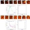 |
Fig. 5 Stacked images of highz and star candidates. b) Fit to the photometric SEDs and the corresponding redshift distribution. The caption of Fig. 4 gives details. |
4.1. The spatial distribution of LBG candidates
Another indication that our selected final LBG candidates are probably not dominated by contaminants is that they are not randomly distributed, but they appear to be concentrated in a specific sky area (Fig. 6). In fact, the distribution of stars is expected to be random, whereas significant asymmetries may be found in the distribution of the high-z galaxies belonging to the quasar structure (e.g., Overzier et al. 2009). We estimated the binomial probability to have 17 or more candidates out of the 21 candidates with RA values smaller than the central QSO, assuming the null hypothesis that they are randomly distributed. We repeat the same calculation for 12 or more out of 21 high-z candidates that populate the north-western (NW) quarter of the field. We obtain a probability of obtaining these asymmetric spatial distributions as low as 0.3% and 0.2%, respectively. If we consider only the candidates robustly classified as highz (i.e., excluding the highz? candidates), in this case the probabilities are 1.% (13 out of 16 candidates in the western half region) and 0.02% (11 out of 16 in the NW quarter of the field). If we do the same exercise considering only the primary sample, the probability is 4% (four out of six of the high-z candidates in the primary sample are in the NW region). In order to test if the asymmetric distribution of the high-z candidates was related to a global variation of objects detected in the field, we divided the parent photometric catalog into four quadrants with the quasar SDSS 1030+0524 as the central point. The density of detected objects in the whole field is remarkably constant, with a relative variation less than 3% of the number of galaxies included in each of the four quadrants. If we restrict such analysis to the reddest objects (with 0.8 < i−z < 1.1), the uniformity holds, albeit with larger variation due to the reduced statistics.
To better quantify whether the spatial distribution of the 21 high-z galaxy candidates differs from a random distribution, we compared their angular correlation function with that of objects classified as contaminants (either stars or low-z galaxies). The two-point angular correlation function w(θ) is defined as the excess probability over random of finding a pair of galaxies in the two small sky areas dΩ1 and dΩ2, separated by an angle θ (Peebles 1980), that is: dP = n2 [1 + w(θ)] dΩ1dΩ2, where n is the mean galaxy density.
To measure w(θ), we used the minimum variance estimator proposed by Landy & Szalay (1993): ![Mathematical equation: \begin{equation} w(\theta)=\frac{[DD]-2[DR]+[RR]}{[RR]}, \end{equation}](/articles/aa/full_html/2017/10/aa30683-17/aa30683-17-eq130.png) (1)where [DD], [DR] and [RR] are the normalized data-data, data-random, and random-random pairs, that is,
(1)where [DD], [DR] and [RR] are the normalized data-data, data-random, and random-random pairs, that is,
![Mathematical equation: \begin{eqnarray} &&[DD]\equiv DD(\theta)\frac{n_{\rm r}(n_{\rm r}-1)}{n_{\rm d}(n_{\rm d}-1)} \\ &&[DR]\equiv DR(\theta)\frac{(n_{\rm r}-1)}{2 n_{\rm d}} \\ &&[RR]\equiv RR(\theta), \end{eqnarray}](/articles/aa/full_html/2017/10/aa30683-17/aa30683-17-eq131.png)
where DD, DR, and RR are the number of data-data, data-random, and random-random pairs at separations θ ± Δθ, and nd and nr are the total number of sources in the data and random sample, respectively. Random sources were distributed across the field according to a spatial mask that follows the geometry of the LBC field of view and removes the same regions excluded when selecting i-band dropouts (e.g., noisy regions around bright stars). Each random sample is built to contain more than 10 000 objects. We considered a range of separations of ~1−30 arcmin and binned the source pairs in intervals of Δlog (θ/ arcmin) = 0.2. As shown in Fig. 7, high-z galaxy candidates show a positive clustering signal (significant at the ~3σ level) on scales ≲10 arcmin, whereas the spatial distribution of the contaminants is fully consistent with random. These results do not change significantly if the most uncertain high-z candidates are removed (i.e., the five objects with a question mark in Table 3). This strongly supports the goodness of our color-morphology classification described in Sect. 4.1.
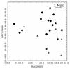 |
Fig. 6 Spatial distribution of our final candidates sample: thick dots represent targets classified in Table 2 as highz galaxies and thin dots are for highz? galaxies. The cross represents the position of the quasar. |
We also fitted to our data a functional form w(θ) = Aw(θ− β−C), where θ is expressed in arcsec, and AwC is the so-called integral constraint, that accounts for the underestimate of w(θ) in finite-size fields. Following Roche & Eales (1999), we computed C using the number of random-random pairs in each angular bin as: 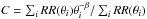 . The best-fit parameters were determined via χ2 minimization. Given the small number of pairs that fall into some bins (especially on the smallest scales), we used the formulae of Gehrels (1986) to estimate the 68% confidence interval (i.e., 1σ errorbars in Gaussian statistics. We fixed β = 0.8, as commonly found in galaxy clustering studies, and found Aw = 40 ± 13 6). This value is more than a dex larger than what is found for the average correlation amplitude of z ~ 6 bright galaxies in blank sky fields (Barone-Nugent et al. 2014; Harikane et al. 2016). Despite the large errors of our measurement, this would further support the existence of a coherent high-z large-scale structure in our field.
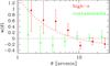 |
Fig. 7 Angular correlation function for the sample of 21 LBG candidates at z ~ 6 (red) and for the sample of 22 contaminants (green, slightly shifted for clarity) of Table 3. A positive (~3σ) signal is measured at θ< 10 arcmin for highz galaxies, whereas a null correlation is observed for the contaminants. The red dashed line is the best fit to the highz galaxy correlation function including the integral constraint. |
4.2. The overdensity of LBGs
We then compared the total number of i-band dropouts observed in the J1030 field with that expected over a blank sky field when using similar photometric bands and images depths, and adopting similar LBG selection criteria. A reference work that satisfies these requirements is that of Bowler et al. (2015). These authors perform a selection of LBGs in the redshift range between 5.5 and 6.5 within a 0.91 deg2 of imaging in the UltraVISTA/Cosmological Evolution Survey (COSMOS) fields and within a 0.74 deg2 imaging in the United Kingdom Infrared Telescope Deep Sky Survey (UKIDSS) Ultra Deep Survey (UDS) fields. They used multi-wavelength data in the optical (u, g, r, i) and near infrared bands (Y, J, H, K), and their selection is based on photometric redshifts. Their images reach a 5σ depth of mAB = 26.7 in the z-band and a 5σ depth of mAB = 25.3 in the Y-band.
Based on the z-band magnitude distribution of our LBG candidates (see, e.g., Fig. 8), we see that our sample is severely incomplete at aperture-corrected magnitudes of zAB > 25.5. To allow a proper comparison with our sample, we therefore considered those LBG candidates of Bowler et al. (2015) at z> 5.7 and with aperture magnitudes of zap< 25.6 7. Based on the histogram in Fig. 6 of Bowler et al. (2015), we counted 61 such objects in their surveyed area of 1.65 deg2. Rescaling for the different area of 0.144 deg2 of our field, we would expect a number of dropouts in our field area of 5.3, whereas we selected 18 candidates with zap< 25.6 (see Fig. 8)8. The Poisson probability of observing 18 or more objects when only 5.3 are expected is 1.2 × 10⁻⁵, corresponding to a significance of >4σ assuming a normal distribution (considering our primary and faint LBG candidate samples separately, we obtained measured overdensity levels of 2 and 3.7σ, respectively). Based on these numbers, we estimate that the J1030 field features an overdensity of z ~ 6 LBGs equal to δ = 2.4 (defined as  , where ρ0 is the expected number counts, see M14 for details). We then confirm and reinforce the overdensity of LBGs found in the J1030 field in M14 (δ = 2.0 at 3.3σ), where we compared the number of i-band dropouts in our field with that measured over the Subaru/XMM Deep Survey after applying the same optical color selection (i−z> 1.4) and after accounting for the different image depths and photometric systems. This suggests that the new selection criteria based on optical/near-IR colors and photometric redshifts have in fact improved the selection of robust LBG candidates.
4.3. Properties of LBG candidates
Finally, we investigated the properties of the highz candidates. The rest-frame UV continuum luminosity results from the integrated light emitted by young stars (mainly O and B massive stars) and it is widely considered as a good proxy of the star formation rate (SFR) in galaxies. At these redshifts, the z-band is very close to rest-frame 1350 Å. We corrected the z-band magnitude for the IGM opacity assuming a UV slope β = −2 (with Fλ = λβ) typical of z ~ 6 dropout galaxies (e.g., Stanway et al. 2005) adopting the Madau (1995) description for the ISM neutral hydrogen absorption. The absolute UV magnitudes were therefore calculated from the corrected z-band magnitudes, assuming z = 6.3. We obtained absolute UV magnitudes in the range −21.3 and −20.5, with a mean value of −20.9 (see Fig. 8). For comparison, the break in the z ~ 6 luminosity function is at MUV = −21 at z ~ 6 (Bouwens et al. 2015). We converted the mean UV luminosity to SFR using the relation of Madau et al. (1998): SFR(M⊙ yr-1) = 1.25 × 10⁻²⁸LUV(erg s-1 Hz-1) valid for a Salpeter (1955) Initial Mass Function (IMF). We obtained SFR ~ 21 M⊙ yr-1 (not corrected for dust absorption of UV light). Conversion to a Kroupa (2001) IMF would result in a factor of ~1.7 smaller SFR estimates. The measured average UV luminosity and SFR are similar to those found by Bowler et al. (2015) in blank sky fields, so we do not find evidence for particularly strong SFRs associated to dense environments as found in some simulations by Yajima et al. (2015).
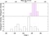 |
Fig. 8 Histogram of the z-band aperture-corrected magnitude for the targets classified as contaminants (in white, lower panel) and for our most promising candidates, that is, the targets classified as highz or highz? in Table 2 (in purple, upper panel). |
4.4. Comparison with previous results
The first indications about the existence of a galaxy overdensity around the QSO SDSS J1030+0524 (within 1.5 arcmin scales) were presented by Stiavelli et al. (2005) and Kim et al. (2009), who analyzed HST/ACS data at z850 < 27 depth and found a ≈2σ excess of objects with i775−z850> 1.3 with respect to what was expected based on the density of sources in the GOODS fields with the same colors and at the same depth. To date, the only HST/ACS i-band dropout in the J1030 field with measured spectroscopic redshift is at z = 5.790 (Stiavelli et al. 2005, confirmed also by Díaz et al. 2011). The search for emission lines in the other ACS/HST dropouts proved inconclusive (Kim et al. 2009). The z = 5.97 object has z850 = 25.74 and is visible in our LBC z-band image, but it falls below our catalog detection threshold. To date, this is the object with redshift closest to that of the QSO. Spectroscopy of a sample of z ~ 5.7 candidate LAEs was presented by Díaz et al. (2015), and the overall redshift range was found to be 5.66 <zspec < 5.75. Only two of these LAEs appear in our LBC catalogs but with colors too blue (i−z = 0.72−0.95) to be selected in any of our dropout samples. In any case, these objects are foreground to the QSO. The radial separation between the z = 5.97 object of Stiavelli et al. (2005) and SDSS J1030+0524 is Δz = 0.34, correponding to ~20 pMpc. This seems larger than the size of the largest galaxy overdensities expected at z ~ 6 (≈10 pMpc; Overzier et al. 2009). Interestingly, the redshift measured in our LBG candidate stack is z = 5.95 ± 0.06. Should this average redshift be confirmed by the forthcoming spectroscopic observations of our targets, this would point towards a z = 5.95−5.97 Large Scale Structure (LSS) that is likely a foreground structure with respect to the QSO.
Further investigations of the environment around SDSS J1030+0524 were presented by D14, who used deep narrow-band (at 8162 Å) and broad band r,i,z imaging obtained with the 30 × 27 arcmin2 Subaru Suprime-Cam to select samples of candidate LAEs and LBGs at z ~ 5.7 (to study the environment of high-z absorbers along the QSO line of sight; D’Odorico et al. 2013) and candidate LBGs at z ~ 6 (selected as i-band dropouts). Their observations cover a FoV that is comparable to (even larger than) our FoV at the same depth, and for their i-band dropout sample they used selection criteria very similar to what we used in M14. It is therefore interesting to compare our findings with that of D14. According to D14, the most significant excess of i-band dropouts is indeed in the NW direction as we found, but it is on scales smaller than 3 arcmin from the QSO, and is made by only three objects. As described in Sect. 6.4.2, and Table 3 of D14, the significance of that excess is ~1.5σ. We verified that five out of the 23 i-band dropouts in the D14 catalog fall in the NW quarter of the LBC field where we find the largest overdensity. The binomial probability of finding five out of 23 objects in that area is 0.3, to be compared with the value of 0.002 that we found in our data. Therefore, our LBC/WIRCAM measurements provide the most significant detection of an overdensity in the J1030 field to date.
To better understand the differences in the i-band dropout samples of D14 and our samples, we also cross matched the source lists. The 23 i-band dropouts of D14 (see their Table E3) are distributed over a wider field, and only 12 of them fall within our field. Five of them are below our z-band detection threshold and hence are not present in our LBC source catalog (M14; most of them appear as low S/N detections in the LBC z-band image though). Among the seven LBC-detected objects, two belong to our primary sample (IDs 11963 and 25831), one to our faint sample (ID 5674), whereas four do not satisfy our color selection criteria. On the one hand, this small overlap can be explained by the somewhat different S/N and colors that we measured in our LBC data. For instance, by slightly relaxing our requirements on the z-band detection significance and i−z color cuts, we would have found five more matches between the i −band dropout samples, bringing the overlap to 8/12. Instead, for the remaining four objects we measured significantly bluer i−z colors than in D14. In some cases the presence of a nearby bright star in LBT images may have affected the accuracy of the photometry and partly explained this color discrepancy. On the other hand, the addition of NIR imaging with WIRCAM (plus Spitzer and MUSYC), allows us to perform a more efficient rejection of contaminants. As a matter of fact, more than half of the primary objects in M14 were found to be contaminants, and their selection closely resembles that of i-band dropouts in D14. In the end, only one of the 12 i-band dropouts of D14 that are covered by our data, namely ID 11963 (see Table 3), was classified by us as highz.
4.5. Comparison with other large-scale overdensities at z ~ 6
The large-scale overdensity measured around SDSS J1030+0524 is one of the few examples of z ~ 6 galaxy overdensities extending on scales larger than 1 pMpc. In most cases, these measurements were performed around z ~ 6 QSOs and based on imaging data only (e.g., Utsumi et al. 2010, M14), and are thus awaiting spectroscopic confirmation. A clear, spectroscopically confirmed overdensity at z = 6.01 has been instead reported by Toshikawa et al. (2012, 2014) in the Subaru Deep Field (SDF, Kashikawa et al. 2004), which does not contain any known luminous QSO at that redshift. By means of imaging data obtained with the wide-field Suprime-Cam at Subaru and subsequent optical spectroscopy at the Keck telecope, Toshikawa et al. (2014) measured an overdensity of i-band dropout that reaches a significance of 6σ at its peak and extends over ~10 × 8 arcmin2, that is, ~3 × 2.2 pMpc2, down to the 2σ level. About 50 i-bands dropouts have been selected by Toshikawa et al. (2014) within this area down to zAB< 27, that is, at limiting fluxes significantly deeper than our data, and for about half of them they were able to measure the redshift through the detection of Lyα emission. The redshifts of their spectroscopic sample cover the range z = 5.7−6.6. Ten objects with average redshift ⟨ z ⟩ = 6.01 were found within a narrow redshift slice of Δz< 0.06 (i.e., within 3.7 pMpc radial), marking an early protocluster structure that is expected to grow into a massive cluster of 5 × 10¹⁴M⊙ by z = 0. Because of the brighter magnitude range covered by our observations (actually Toshikawa et al. excluded all the i-band dropout with z< 25 from their analysis), it is difficult to compare the candidate overdensity we measured in the J1030 field with that measured in the SDF. We note, however, that the angular scales over which we measure the highest density of dropouts, that is, the NW quadrant, is ~12 × 12 arcmin2, that is, it has a similar size to the structure measured in the SDF. A more detailed comparison will be possible after spectroscopic observations of our i-band dropout targets.
5. Summary and conclusions
The ultimate goal of this series of papers is to investigate the properties of the environment of high redshift SMBHs that, according to cosmological simulations, should be characterized by large overdensities of primordial galaxies. In M14 we selected a catalog of i-dropout candidates around four high redshift quasars using wide-field LBT images in r, i, and z bands.
Here we present deep-and-wide (~25′ × 25′) Y- and J-band images obtained with the near infrared camera WIRCam at CFHT around one of these quasars, SDSS 1030+0524 at z = 6.31. The field of view, the resolution, and the sensitivity match the LBT observations. We use these new data to improve the selection of LBG candidates, rejecting potential contaminants (stars or galaxies at lower redshift). With respect to M14, we added 18 new faint candidates using a color criterion similar to the one adopted for primary candidates (i−z> 1.3), but applied to fainter objects (25.2 <zAB< 25.7).
We estimated the photometric redshifts of the objects in the primary, secondary, and faint samples by fitting their SEDs from ~0.9 to 3.2 μm, using our own photometric data in the r, i,z, Y, and J bands and, if available, also those in the H and K bands (from the MUSYC survey) and at 3.4 and 4.5 μm (from public Spitzer/IRAC data). We evaluated the position of each target in the (i−z) versus (z−Y) color-color diagnostic plot and made a robust morphology classification. We combined all this information to divide the objects in our samples into reliable LBG candidates at z ~ 6 (highz) or contaminants (star or galaxy), and we finally identify a sample of 21 trustable high-z objects.
To confirm the goodness of our selection method, we performed several tests: 1) we stacked the images of the 21 highz and of the 17 objects classified as stars and measured the rizYJ magnitudes in the stacks. The colors and the best fit SEDs of the two stacks are very different. The stack of star-like objects is indeed well fit by a stellar template at z = 0, whereas the stack of highz candidates is well fit by an LBG template at zphot = 5.95 ± 0.06; 2) we investigated the clustering properties of the two populations. We observed a clear asymmetric spatial distribution for the highz candidates in the field, which is significant at the >3σ level. We also verified that the angular correlation function of highz shows a significant positive signal at scales <10 arcmin, wheres the angular correlation function of stars is consistent with zero, suggesting that these objects are randomly distributed in the field, as indeed expected for galactic stars. The strong clustering signal measured for the 21 highz objects instead again suggests the presence of a coherent high-z large-scale structure in the field.
We finally compared the number of robust z ~ 6 LBG candidates with that observed by Bowler et al. (2015) in blank sky fields, which was obtained by applying similar selection methods. We measured an LBG overdensity of δ = 2.4 that is significant at the >4σ level. We therefore confirm and reinforce the high-z galaxy overdensity reported by M14. We are planning spectroscopic observations of these LBG candidates in the next months to confirm whether they are actually at the same redshift of the quasar.
Terapix is an astronomical data reduction centre dedicated to the processing of data from various telescopes and optical or near infrared cameras, such as WIRCam.
The completeness limit was defined as the magnitude at which the number of detected objects fall at 50% of the expected value.
See page 64 of the IRAC Instrument Handbook.
We assume Gaussian error since in Gilli et al. (2005, 2009) we verified that bootstrap errors are on average a factor of two higher than the simple 1σ errors. If we assume bootstrap errors, we obtain a clustering signal still significant within ~2σ level.
Bowler et al. use apertures similar to ours for the photometry (1.8 versus 1.6 arcsec diameter) and their data have been taken under similar seeing conditions, so we expect aperture corrections similar to those we found in M14, that is, Δmag ~ 0.1.
Bowler et al. found a factor of two of difference between the counts in Ultravista/COSMOS and UDS/XDS. At the magnitude limits z = 25.6, this factor reduces to ~1.5, corresponding to a maximum of 7.6 objects expected in our 0.144 deg2 area versus the 18 observed at that limit. Even conservatively assuming this high “background” value, the overdensity in the J030 field would be significant at more than 3σ.
Acknowledgments
We are grateful to the referee for the careful reading of the manuscript and for the useful comments. We acknowledge financial contribution from the agreement ASI-INAF I/037/12/0. F.V. acknowledges support from Chandra X-ray Center grant GO4-15130A and the V.M. Willaman Endowment. This work is based on observations obtained with WIRCam, a joint project of CFHT, Taiwan, Korea, Canada, and France, at the Canada-France-Hawaii Telescope (CFHT) which is operated by the National Research Council (NRC) of Canada, the Institut National des Sciences de l’Univers of the Centre National de la Recherche Scientifique of France, and the University of Hawaii. Based on observations obtained with MegaPrime/MegaCam, a joint project of CFHT and CEA/DAPNIA, at the Canada-France-Hawaii Telescope (CFHT) which is operated by the National Research Council (NRC) of Canada, the Institut National des Sciences de l’Univers of the Centre National de la Recherche Scientifique (CNRS) of France, and the University of Hawaii. This work is based in part on data products produced at TERAPIX and the Canadian Astronomy Data Centre as part of the Canada-France-Hawaii Telescope Legacy Survey, a collaborative project of NRC and CNRS.
References
- Angulo, R. E., Hahn, O., & Abel, T. 2013, MNRAS, 434, 1756 [NASA ADS] [CrossRef] [Google Scholar]
- Babul, A., & White, S. D. M. 1991, MNRAS, 253, 31 [NASA ADS] [Google Scholar]
- Barone-Nugent, R. L., Trenti, M., Wyithe, J. S. B., et al. 2014, ApJ, 793, 17 [NASA ADS] [CrossRef] [Google Scholar]
- Beckwith, S. V. W., Stiavelli, M., Koekemoer, A. M., et al. 2006, AJ, 132, 1729 [NASA ADS] [CrossRef] [Google Scholar]
- Blanc, G. A., Lira, P., Barrientos, L. F., et al. 2008, ApJ, 681, 1099 [NASA ADS] [CrossRef] [Google Scholar]
- Bolzonella, M., Miralles, J.-M., & Pelló, R. 2000, A&A, 363, 476 [NASA ADS] [Google Scholar]
- Bouwens, R. J., Illingworth, G. D., Oesch, P. A., et al. 2015, ApJ, 811, 140 [NASA ADS] [CrossRef] [Google Scholar]
- Bowler, R. A. A., Dunlop, J. S., McLure, R. J., et al. 2015, MNRAS, 452, 1817 [NASA ADS] [CrossRef] [Google Scholar]
- Brodwin, M., Lilly, S. J., Porciani, C., et al. 2006, ApJS, 162, 20 [NASA ADS] [CrossRef] [Google Scholar]
- Bruzual, A. G., & Charlot, S. 1993, ApJ, 405, 538 [NASA ADS] [CrossRef] [Google Scholar]
- Calzetti, D., Armus, L., Bohlin, R. C., et al. 2000, ApJ, 533, 682 [NASA ADS] [CrossRef] [Google Scholar]
- Coleman, G. D., Wu, C.-C., & Weedman, D. W. 1980, ApJS, 43, 393 [NASA ADS] [CrossRef] [Google Scholar]
- Costa, T., Sijacki, D., Trenti, M., & Haehnelt, M. G. 2014, MNRAS, 439, 2146 [NASA ADS] [CrossRef] [Google Scholar]
- Di Matteo, T., Khandai, N., DeGraf, C., et al. 2012, ApJ, 745, L29 [NASA ADS] [CrossRef] [Google Scholar]
- Díaz, C. G., Ryan-Weber, E. V., Cooke, J., Pettini, M., & Madau, P. 2011, MNRAS, 418, 820 [NASA ADS] [CrossRef] [Google Scholar]
- Díaz, C. G., Koyama, Y., Ryan-Weber, E. V., et al. 2014, MNRAS, 442, 946 [NASA ADS] [CrossRef] [Google Scholar]
- Díaz, C. G., Ryan-Weber, E. V., Cooke, J., Koyama, Y., & Ouchi, M. 2015, MNRAS, 448, 1240 [NASA ADS] [CrossRef] [Google Scholar]
- Dickinson, M., Stern, D., Giavalisco, M., et al. 2004, ApJ, 600, L99 [NASA ADS] [CrossRef] [Google Scholar]
- D’Odorico, V., Cupani, G., Cristiani, S., et al. 2013, MNRAS, 435, 1198 [NASA ADS] [CrossRef] [Google Scholar]
- Dunlop, J. S. 2013, in The First Galaxies, eds. T. Wiklind, B. Mobasher, & V. Bromm, Astrophys. Space Sci. Libr., 396, 223 [Google Scholar]
- Finkelstein, S. L. 2016, PASA, 33, e037 [NASA ADS] [CrossRef] [Google Scholar]
- Garcia-Vergara, C., Hennawi, J. F., Barrientos, L. F., & Rix, H.-W. 2017, ArXiv e-prints [arXiv:1701.01114] [Google Scholar]
- Gehrels, N. 1986, ApJ, 303, 336 [NASA ADS] [CrossRef] [Google Scholar]
- Gilli, R., Daddi, E., Zamorani, G., et al. 2005, A&A, 430, 811 [NASA ADS] [CrossRef] [EDP Sciences] [Google Scholar]
- Gilli, R., Zamorani, G., Miyaji, T., et al. 2009, A&A, 494, 33 [NASA ADS] [CrossRef] [EDP Sciences] [Google Scholar]
- Harikane, Y., Ouchi, M., Ono, Y., et al. 2016, ApJ, 821, 123 [NASA ADS] [CrossRef] [Google Scholar]
- Husband, K., Bremer, M. N., Stanway, E. R., et al. 2013, MNRAS, 432, 2869 [NASA ADS] [CrossRef] [Google Scholar]
- Ilbert, O., Arnouts, S., McCracken, H. J., et al. 2006, A&A, 457, 841 [NASA ADS] [CrossRef] [EDP Sciences] [Google Scholar]
- Inoue, A. K., Shimizu, I., Iwata, I., & Tanaka, M. 2014, MNRAS, 442, 1805 [NASA ADS] [CrossRef] [Google Scholar]
- Kashikawa, N., Shimasaku, K., Yasuda, N., et al. 2004, PASJ, 56, 1011 [NASA ADS] [CrossRef] [Google Scholar]
- Kashikawa, N., Kitayama, T., Doi, M., et al. 2007, ApJ, 663, 765 [NASA ADS] [CrossRef] [Google Scholar]
- Kim, S., Stiavelli, M., Trenti, M., et al. 2009, ApJ, 695, 809 [NASA ADS] [CrossRef] [Google Scholar]
- Kinney, A. L., Calzetti, D., Bohlin, R. C., et al. 1996, ApJ, 467, 38 [NASA ADS] [CrossRef] [Google Scholar]
- Kroupa, P. 2001, MNRAS, 322, 231 [NASA ADS] [CrossRef] [Google Scholar]
- Landy, S. D., & Szalay, A. S. 1993, ApJ, 412, 64 [NASA ADS] [CrossRef] [Google Scholar]
- Madau, P. 1995, ApJ, 441, 18 [NASA ADS] [CrossRef] [Google Scholar]
- Madau, P., Pozzetti, L., & Dickinson, M. 1998, ApJ, 498, 106 [NASA ADS] [CrossRef] [Google Scholar]
- Matsuoka, Y., Onoue, M., Kashikawa, N., et al. 2016, ApJ, 828, 26 [NASA ADS] [CrossRef] [Google Scholar]
- Mazzucchelli, C., Bañados, E., Decarli, R., et al. 2017, ApJ, 834, 83 [NASA ADS] [CrossRef] [Google Scholar]
- Meiksin, A. 2006, MNRAS, 365, 807 [NASA ADS] [CrossRef] [Google Scholar]
- Morselli, L., Mignoli, M., Gilli, R., et al. 2014, A&A, 568, A1 [NASA ADS] [CrossRef] [EDP Sciences] [Google Scholar]
- Mortlock, D. J. 2016, Astrophys. Space Sci. Lib., 423, 187 [NASA ADS] [CrossRef] [Google Scholar]
- Overzier, R. A. 2016, A&ARv, 24, 14 [NASA ADS] [CrossRef] [Google Scholar]
- Overzier, R. A., Guo, Q., Kauffmann, G., et al. 2009, MNRAS, 394, 577 [NASA ADS] [CrossRef] [Google Scholar]
- Peebles, P. J. E. 1980, The large-scale structure of the universe (Princeton, N.J.: Princeton University Press) [Google Scholar]
- Polletta, M., Tajer, M., Maraschi, L., et al. 2007, ApJ, 663, 81 [NASA ADS] [CrossRef] [Google Scholar]
- Quadri, R., Marchesini, D., van Dokkum, P., et al. 2007, AJ, 134, 1103 [NASA ADS] [CrossRef] [Google Scholar]
- Rees, M. J. 1988, in Large Scale Structures of the Universe, eds. J. Audouze, M.-C. Pelletan, A. Szalay, Y. B. Zel’dovich, & P. J. E. Peebles, IAU Symp., 130, 437 [Google Scholar]
- Roche, N., & Eales, S. A. 1999, MNRAS, 307, 703 [NASA ADS] [CrossRef] [Google Scholar]
- Salpeter, E. E. 1955, ApJ, 121, 161 [Google Scholar]
- Schlegel, D. J., Finkbeiner, D. P., & Davis, M. 1998, ApJ, 500, 525 [NASA ADS] [CrossRef] [Google Scholar]
- Simpson, C., Mortlock, D., Warren, S., et al. 2014, MNRAS, 442, 3454 [NASA ADS] [CrossRef] [Google Scholar]
- Stanway, E. R., McMahon, R. G., & Bunker, A. J. 2005, MNRAS, 359, 1184 [NASA ADS] [CrossRef] [Google Scholar]
- Steidel, C. C., Giavalisco, M., Pettini, M., Dickinson, M., & Adelberger, K. L. 1996, ApJ, 462, L17 [NASA ADS] [CrossRef] [Google Scholar]
- Stiavelli, M., Djorgovski, S. G., Pavlovsky, C., et al. 2005, ApJ, 622, L1 [NASA ADS] [CrossRef] [Google Scholar]
- Toshikawa, J., Kashikawa, N., Ota, K., et al. 2012, ApJ, 750, 137 [NASA ADS] [CrossRef] [Google Scholar]
- Toshikawa, J., Kashikawa, N., Overzier, R., et al. 2014, ApJ, 792, 15 [NASA ADS] [CrossRef] [Google Scholar]
- Utsumi, Y., Goto, T., Kashikawa, N., et al. 2010, ApJ, 721, 1680 [NASA ADS] [CrossRef] [Google Scholar]
- Vanzella, E., Giavalisco, M., Dickinson, M., et al. 2009, ApJ, 695, 1163 [NASA ADS] [CrossRef] [Google Scholar]
- Willott, C. J., McLure, R. J., Hibon, P., et al. 2013, AJ, 145, 4 [NASA ADS] [CrossRef] [Google Scholar]
- Wu, X.-B., Wang, F., Fan, X., et al. 2015, Nature, 518, 512 [NASA ADS] [CrossRef] [PubMed] [Google Scholar]
- Yajima, H., Shlosman, I., Romano-Díaz, E., & Nagamine, K. 2015, MNRAS, 451, 418 [NASA ADS] [CrossRef] [Google Scholar]
Appendix
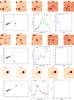 |
Fig. A.1 Full version of Fig. 4. |
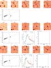 |
Fig. A.1 continued. |
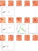 |
Fig. A.1 continued. |
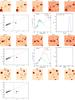 |
Fig. A.1 continued. |
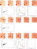 |
Fig. A.1 continued. |
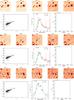 |
Fig. A.1 continued. |
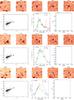 |
Fig. A.1 continued. |
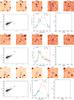 |
Fig. A.1 continued. |
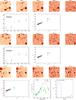 |
Fig. A.1 continued. |
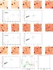 |
Fig. A.1 continued. |
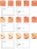 |
Fig. A.1 continued. |
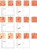 |
Fig. A.1 continued. |
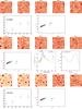 |
Fig. A.1 continued. |
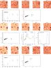 |
Fig. A.1 continued. |
All Tables
Multi-band photometry for the sample LBG primary, secondary and faint candidates.
Colors, morphology, photometric redshift and final classification for our candidates.
All Figures
|
Fig. 1 Response filter curves of the WIRCam camera in the Y- and J-bands and for LBT/LBC r, i, and z bands (SDSS-like filters). We show in red a star-forming galaxy template at z = 6.3 with age 0.5 Gyr and Z = 0.02Z⊙ (from Bruzual & Charlot 2003) and in green a template of a T-type dwarf star from the SpeX Prism Spectral Libraries. |
| In the text | |
|
Fig. 2 CFHT/WIRCam Y and J two-color-composite image of the 1030 field. The image is ~24′ × 24′ and covers the entire LBT/LBC field of view (FoV). North is up and east is to the left. The central SDSS QSO at z = 6.31 is shown as a magenta circle. The LBG primary and secondary i-band dropouts of M14 are shown as red and green circles, respectively. Blue circles mark the new faint candidates (see text for details). |
| In the text | |
|
Fig. 3 Diagnostic (z−Y) versus (i−z) color-color diagram. Small gray dots are point-like sources in the J1030 field (star locus). Red, green, and cyan are the primary and secondary candidates of M14 and the new faint candidates, respectively. For those objects that are not detected at the 2σ level in i or in Y, we used the 2σ local limiting magnitudes. The limits on their colors are marked with arrows. The black curve shows the expected color track (in steps of Δz = 0.1, starting from 5.5) of a high-z star-forming galaxy with age 0.5 Gyr and Z = 0.02 Z⊙ (from Bruzual & Charlot 2003). The gray curve has been calculated with the same template but with an intrinsic absorption Av equal to one and the green curve adding to the template a Lyα emission line with EW = 100 Å rest frame. The blue curve shows the expected color track of a Type 1 QSO (template from the SWIRE library). Objects that have now been classified as reliable z ~ 6 LBGs (see Table 3 and Sect. 4) are marked with large black open circles. The bigger magenta circle and the diamond symbol represent the colors of the stack of the LBG candidates and stellar contaminants, respectively. The blue point marks the position of the central QSO SDSS J1030+0524 at z = 6.31. |
| In the text | |
|
Fig. 4 Example of our classification strategy based on morphology, colors, and photometric redshift for two z ~ 6 LBG candidates in the J1030 field, that we respectively classified as likely star (upper panel) and highz objects (lower panel). Upper panel (same for the lower panel): a) postage stamps (7′′ on a side) in the r, i, z, Y, J, IRAC/ch1, IRAC/ch2 filters. We note that the apparent mismatch of the point sources in the IRAC images is due to the lack of Spitzer data for some targets. b) Photometric colors diagnostic plot. The small black dots are stars in the field and the dashed line represents an extrapolation of the stellar locus based on the colors of known M, L, and T-type dwarfs. The red point represents the color of the LBG candidate. c) SED fitting and photometric redshift determination for the same candidate. Blue squares represent AB magnitudes in r, i, z, Y, J, and Spitzer/IRAC ch1 and ch2 bands with 1σ-error. The best fit is shown with a red line for galaxy and with a green line for stellar case solutions. We report the χ2 for the two template solutions. d) Corresponding probability distribution of the best fit as a function of redshift. We present these summary plots for all the candidates in Appendix A. |
| In the text | |
|
Fig. 5 Stacked images of highz and star candidates. b) Fit to the photometric SEDs and the corresponding redshift distribution. The caption of Fig. 4 gives details. |
| In the text | |
|
Fig. 6 Spatial distribution of our final candidates sample: thick dots represent targets classified in Table 2 as highz galaxies and thin dots are for highz? galaxies. The cross represents the position of the quasar. |
| In the text | |
|
Fig. 7 Angular correlation function for the sample of 21 LBG candidates at z ~ 6 (red) and for the sample of 22 contaminants (green, slightly shifted for clarity) of Table 3. A positive (~3σ) signal is measured at θ< 10 arcmin for highz galaxies, whereas a null correlation is observed for the contaminants. The red dashed line is the best fit to the highz galaxy correlation function including the integral constraint. |
| In the text | |
|
Fig. 8 Histogram of the z-band aperture-corrected magnitude for the targets classified as contaminants (in white, lower panel) and for our most promising candidates, that is, the targets classified as highz or highz? in Table 2 (in purple, upper panel). |
| In the text | |
|
Fig. A.1 Full version of Fig. 4. |
| In the text | |
|
Fig. A.1 continued. |
| In the text | |
|
Fig. A.1 continued. |
| In the text | |
|
Fig. A.1 continued. |
| In the text | |
|
Fig. A.1 continued. |
| In the text | |
|
Fig. A.1 continued. |
| In the text | |
|
Fig. A.1 continued. |
| In the text | |
|
Fig. A.1 continued. |
| In the text | |
|
Fig. A.1 continued. |
| In the text | |
|
Fig. A.1 continued. |
| In the text | |
|
Fig. A.1 continued. |
| In the text | |
|
Fig. A.1 continued. |
| In the text | |
|
Fig. A.1 continued. |
| In the text | |
|
Fig. A.1 continued. |
| In the text | |
Current usage metrics show cumulative count of Article Views (full-text article views including HTML views, PDF and ePub downloads, according to the available data) and Abstracts Views on Vision4Press platform.
Data correspond to usage on the plateform after 2015. The current usage metrics is available 48-96 hours after online publication and is updated daily on week days.
Initial download of the metrics may take a while.