| Issue |
A&A
Volume 606, October 2017
|
|
|---|---|---|
| Article Number | A145 | |
| Number of page(s) | 13 | |
| Section | Stellar structure and evolution | |
| DOI | https://doi.org/10.1051/0004-6361/201630119 | |
| Published online | 26 October 2017 | |
XMM-Newton spectroscopy of the accreting magnetar candidate 4U0114+65
1 Instituto de Físca Aplicada a las Ciencias y las Tecnologías, Universidad de Alicante, 03690 Alicante, Spain
e-mail: This email address is being protected from spambots. You need JavaScript enabled to view it.
2 Sternberg Astronomical Institute, Moscow M.V. Lomonosov State University, Universitetskij pr., 13, 119234 Moscow, Russia
3 Institute for Physics and Astronomy, Universität Potsdam, 14476 Potsdam, Germany
Received: 22 November 2016
Accepted: 6 June 2017
Abstract
Aims. 4U0114+65 is one of the slowest known X-ray pulsars. We present an analysis of a pointed observation by the XMM-Newton X-ray telescope in order to study the nature of the X-ray pulsations and the accretion process, and to diagnose the physical properties of the donor’s stellar wind.
Methods. We analysed the energy-resolved light curve and the time-resolved X-ray spectra provided by the EPIC cameras on board XMM-Newton. We also analysed the first high-resolution spectrum of this source provided by the Reflection Grating Spectrometer.
Results. An X-ray pulse of 9350 ± 160 s was measured. Comparison with previous measurements confirms the secular spin up of this source. We successfully fit the pulse-phase-resolved spectra with Comptonisation models. These models imply a very small (r ~ 3 km) and hot (kT ~ 2 − 3 keV) emitting region and therefore point to a hot spot over the neutron star (NS) surface as the most reliable explanation for the X-ray pulse. The long NS spin period, the spin-up rate, and persistent X-ray emission can be explained within the theory of quasi-spherical settling accretion, which may indicate that the magnetic field is in the magnetar range. Thus, 4U 0114+65 could be a wind-accreting magnetar. We also observed two episodes of low luminosity. The first was only observed in the low-energy light curve and can be explained as an absorption by a large over-dense structure in the wind of the B1 supergiant donor. The second episode, which was deeper and affected all energies, may be due to temporal cessation of accretion onto one magnetic pole caused by non-spherical matter capture from the structured stellar wind. The light curve displays two types of dips that are clearly seen during the high-flux intervals. The short dips, with durations of tens of seconds, are produced through absorption by wind clumps. The long dips, in turn, seem to be associated with the rarefied interclump medium. From the analysis of the X-ray spectra, we found evidence of emission lines in the X-ray photoionised wind of the B1Ia donor. The Fe Kα line was found to be highly variable and much weaker than in other X-ray binaries with supergiant donors. The degree of wind clumping, measured through the covering fraction, was found to be much lower than in supergiant donor stars with earlier spectral types.
Conclusions. The XMM-Newton spectroscopy provided further support for the magnetar nature of the neutron star in 4U0114+65. The light curve presents dips that can be associated with clumps and the interclump medium in the stellar wind of the mass donor.
Key words: X-rays: binaries / stars: winds, outflows / pulsars: individual: 4U0114+65
© ESO, 2017
1. Introduction
High-mass X-ray binaries (HMXBs) are systems formed by a compact object (i.e. a neutron star or a black hole) orbiting a massive star (the companion). These are excellent laboratories where the process of accretion and the structure of the companion’s stellar wind can be studied (Martínez-Núñez et al. 2017). The source 4U 0114+65 was discovered by (Dower et al. 1977) in the SAS 3 Galactic survey. The donor star is V∗ V662 Cas, a luminous BI1a supergiant (Reig et al. 1996) showing significant temporal and spectral variability over a wide range of timescales (Crampton et al. 1985). With an orbital period of ~ 11.6 d, the neutron star (NS) orbits the donor deeply embedded into its wind at an orbital radius of a ≈ [ 1.34 − 1.65 ] R∗ (see Table 1 and Fig. 1), thereby offering the opportunity to probe the inner wind of the B1 supergiant star. Other systems with similar donor spectral types but different orbital parameters are Vela X-1 (V∗ GP Vel, B0.5Ia) or 4U 1538−52 (QV Nor, B0.5Ib).
The source 4U 0114+65 is a non-eclipsing system (Pradhan et al. 2015) and hosts an X-ray pulsar with a ~ 2.6 h spin period, which makes it one of the slowest known X-ray pulsars. In order to explain such a slow spin period, (Li & van den Heuvel 1999) suggested that this object could have been born as a magnetar. Magnetars are neutron stars powered by their strong magnetic dipole fields, B ≃ 1014 − 1015G (Duncan & Thompson 1992), and they can be present in HMXBs (Bozzo et al. 2008). The pulse period of 4U 0114+65 has been changing fast over the years. It was first measured to be ~2.78 h by (Finley et al. 1992). Eight years later, (Hall et al. 2000) measured a period of ~2.73 h, but in 2005, (Bonning & Falanga 2005) obtained a spin period of ~2.67 h. A year later, (Farrell et al. 2006) obtained a spin period of ~2.65 h. (Wang 2011) also discovered a spin period evolution from ~2.67 h to 2.63 h between 2003 and 2008, with a spin-up rate of the neutron star of ~1.09 ×10⁻⁶ s-1. In Table 2 we compile all the spin periods measured to date.
Long periods of X-ray pulsars suggest high magnetic fields of accreting NS (Ikhsanov & Beskrovnaya 2013). As an alternative (Koenigsberger et al. 2006) proposed that the periodicities in this system could be explained by the accretion of a structured wind produced by tidally driven oscillations in the B-supergiant star photosphere induced by the closely orbiting NS.
Velocity of the stellar wind, calculated with a β-law equation:  , with the value β = 0.8 (Lamers & Cassinelli 1999), at the site of the NS.
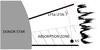 |
Fig. 1 Sketch of the system where we can compare the size of the donor star with the orbit (NS size not to scale). The light curve is displayed parallel to the orbit. |
In this paper we present an analysis of a 49 ks XMM-Newton pointed observation, which represents the longest uninterrupted observation performed so far for this source using modern CCD1 X-ray telescopes.
2. Observations and analysis
We observed 4U 0114+65 for 49 ks using the X-ray Multi-Mirror Mission (XMM-Newton), launched by the European Space Agency (ESA) on December 10, 1999. XMM-Newton carries three high throughput X-ray telescopes and one optical monitor. The three EPIC instruments contain imaging detectors covering the energy range 0.15–10 keV with moderate spectral resolution. The two EPIC MOS cameras and the EPIC PN instrument were operated in small-window mode in order to avoid any pile-up. A thin filter was used to avoid optical load.
The observations were carried out in the time interval between 21-05-2015 20:43:19 UT MJD =57 163.8634 and 22-05-2015 10:01:53 UT, corresponding to an average orbital phase φ≈0.7 (using a Porb=11.5983 d and the ephemeris of Pradhan et al. 2015), which covers approximately 5% of the orbit. Our XMM-Newton observation was performed well outside the minimum in the long-term light curve (see Pradhan et al. 2015 for Suzaku observations performed during the minimun). The data can be found in the XMM archive under the ID 0764650101. The EPIC data were reduced using the Science Analysis Software v5.3.3 (SAS). The data were first processed through the pipeline chains and filtered. For EPIC MOS, only events with a pattern between 0 and 12 were considered, filtered through #XMMEA EM. For EPIC PN, we kept events with flag = 0 and a pattern between 0 and 4 (Strüder et al. 2001). We also checked whether the observations were affected by pile-up using the task epatplot, with negative results. For the spectral analysis we combined the data of the three EPIC cameras (MOS1, MOS2, and PN) into one single spectrum using the task epicspeccombine. The spectra were analysed and modelled with the XSPEC package2. The emission lines were identified thanks to the ATOMBD3 data base. On the other hand, the light-curve timing analysis was performed only on the PN data because of its higher time resolution. The photon arrival times were transformed to the solar system barycenter. To analyse the light curves, we used the period task inside the Starlink suite4.
The Reflection Grating Spectrometer RGS data were processed through the rgsproc pipeline SAS meta-task. This routine determines the location of the source spectrum on the detector, and performs the extraction of the source spectrum as well as of the background spectrum from a spatially offset background region. Finally, the task computes tailored response matrices for the first and second order. Both orders for RGS 1 and 2 were combined for the spectral analysis, providing a high-resolution spectrum in the energy range from 0.33 to 2.13 keV for the first time.
3. Results
3.1. Light curve and pulse period
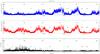 |
Fig. 2 Light curve in two different energy ranges: upper panel 0.3–3.0 keV, and middle panel 3–10 keV. The lower panel shows the colour ratio (3–10) keV/(0.3–3.0) keV. The vertical green line divides T1 and T2 time intervals. The labels LF5a and LF5b refer to low-flux intervals, see text for detail. The epoch time corresponds to 57 255.50 MJD. |
Compilation of spin period measured from 1992 until the present.
The low-energy (0.3–3 keV) and high-energy (3.0–10 keV) light curves of the source are presented in Fig. 2 along with their ratio. The light curves clearly show a main pulse, in addition to which the stochastic variability, typical of wind accretion, can be seen, revealing the complexity of the accretion process. There is a strong pulse-to-pulse variability. The three and a half first pulses are similar in duration and in shape, whereas the last two pulses are very different. From now on, we refer to the three first pulses as T1 and to the last two pulses as T2.
We performed time-resolved spectroscopy to divide the light curve into time bins corresponding to high flux (HF) and low flux (LF) states, respectively. These intervals are shown in Fig. 2 in chronological order (note that LF5 is additionally divided into LF5a and LF5b because LF5 is much longer than the other low-flux states). The duration of the low and high states is not constant (see Fig. 2).
The light curve is complex, therefore we used only the T1 interval and restricted the analysis to the high-energy range, from 8 keV to 10 keV, where the photoelectric absorption effects would be negligible, to compute a reliable spin period. We calculated the spin period using several techniques. The Lomb-Scargle method redefines the classical periodogram in such a manner as to make it invariant to a shift of the origin of time (Lomb 1976; Scargle 1982). The Fourier method performs a classical discrete Fourier transform on the data and sums the mean-square amplitudes of the result to form a power spectrum. The Clean algorithm basically deconvolves the spectral window from the discrete Fourier power spectrum (or dirty spectrum), producing a clean spectrum, which is largely free of the many effects of spectral leakage (Roberts et al. 1987). Finally, we calculated the time separation between consecutive low states as another measure of the spin period. We chose the low states because they show less variability than the high states. First we selected the time intervals with fewer than 6.5 counts/s, then we fitted these data to a Gaussian distribution, calculated the mean number of counts/s and rejected all of the counts beyond the two-sigma range. Then we rejected the outliers outside of the low states following the same method. The results are shown in Table 3. Clearly, all the results are consistent. The associated errors are relatively large because the light curve covers only 3.5 cycles of the pulse period.
Pulse period obtained with different methods.
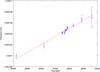 |
Fig. 3 Evolution of the pulse frequency from 1986 to 2015. |
We finally computed the weighted average of pulse periods and determined a spin period of 9350 ± 160 s where the uncertainty corresponds to the weighted error. In order to check this result and increase the reliability of the pulse derivative, we also analysed a longer archival Suzaku light curve (2011-07-21 10:20:15, covering 12 cycles) using the same Starlink tools as described before. The derived period is given in Table 2. The historic period evolution is shown in Fig. 3. The frequency derivative is  Hz s-1. Our observation is consistent with the secular spin-up trend of the pulsar5. We can also derive the pulse period at the time of our XMM-Newton observation using the historical trend. The result is 9320 ± 1 s, consistent with our previous determination (Table 3). Subsequently, we folded the light curve to the pulse period derived from the historical trend (9320 ± 1 s; Fig. 4). As expected, the pulse shape changes from T1 to T2. We compared the folded pulse with the pulses obtained in previous studies that were performed at different orbital phases. Our T1 folded pulse (blue line in Fig. 4) is very similar to the folded pulse obtained by Finley et al. (1992; at φorb = 0.36). On the other hand, our T2 pulse is similar to the pulses obtained by (Farrell et al. 2006), whose observations covered all orbital phases (as they lasted 2.6 orbital cycles each). The source shows pulse shape changes that are unrelated with the orbital phase.
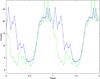 |
Fig. 4 0.3–10 keV light curve, folded on the spin period (9320 ± 1 s), for T1 (blue solid line) and T2 (green dashed line). The epoch time is 57 255.50 MJD. |
Finally, during the whole observation, but specially during the HF states, we identify sharp drops in the flux on rather short timescales, so-called dips. We carefully checked for any periodicity associated with these dips to ensure that they are not related to a potential short-pulse period. The periodograms, however, do not show any significant peaks. We conclude that the dips are stochastic in nature.
A close inspection shows that there are two types of dips: short, with typical durations of several tens of seconds, and long, lasting several hundreds of seconds. In Fig. 5 we mark them with vertical lines (green for short dips and magenta for long dips) for HF2 and HF6, where the dips are seen more clearly. The durations of the dips are ~ 70 ± 30 s (short) and ~ 530 ± 110 s (long). In the long dips the colour ratio tends to remain constant. Only two out of nine of the long dips show an increase in the CR. In the short dips, in turn, five out of six show a CR increase6.
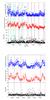 |
Fig. 5 Detailed view of two light curve sections, HF2 (top panel) and HF6 (bottom panel). Each panel is additionally subdivided into three divisions. The upper division corresponds to the low-energy light curve, the middle division to the high-energy light curve, and the lower division to the colour ratio. The short and long dips are marked by green and magenta lines, respectively. |
3.2. EPIC spectrum
We performed time-resolved spectroscopy for each HF and LF state seen in the light curve. The continuum was described using the bulk motion Comptonisation (bmc) model. This is an analytical model that describes the Comptonisation of soft seed photons by matter undergoing relativistic bulk motion (Titarchuk et al. 1997). The model parameters are the characteristic black-body temperature of the soft photon source, a spectral (energy) index (α), and an illumination parameter characterizing the fractional illumination of the bulk motion flow by the thermal photon source.
The absortion is modelled by the Tuebingen-Boulder interstellar medium (ISM) absorption model Tbabs. This model calculates the cross-section for X-ray absorption by the ISM as the sum of the cross-sections that are due to the gas-phase ISM, the grain-phase ISM, and the molecules in the ISM (Wilms et al. 2000). The continuum is modified at low energies by a partial covering absorber in order to account for the wind clumping of the donor star, estimated through the partial covering fraction (parameter C). Emission lines at 6.4 keV (Fe Kα fluorescence), 0.78 keV (Fe xviii), 0.42 keV (N vi He-like), and 0.38 keV (Cv Lyman α) are clearly detected. We modelled them as Gaussians, with a fixed width of 50 eV, while their norms were allowed to vary. The complete model is described by the equation 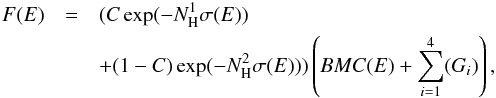 (1)where Gi represent the Gaussians describing the emission lines. In Table A.1 we show the best-fit parameters. The reduced χ2 value is below 1.2 in most of the time bins, except in LF1, HS4, and HS5. In LF1 the high value of χ2 is due to instrumental features that are only present in the EMOS2 spectrum. On the other hand, the high χ2 value of HS4 and HS5 is due mostly to residuals around the Au edge. The high value of χ2 of the average spectrum (Fig. 7) is expected because of the high variability of the source.
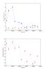 |
Fig. 6 Evolution of the density columns (top) and radius of the seed soft photon source (bottom) for the bmc model. The top panel shows that the first-component absorption (red line) remains constant, compatible wih the ISM medium. The blue line represents the absorption of the ISM plus the circum-source environment, which changes during the observation. It is particularly high at the beginning of the observation, when the low-energy light curve is partially suppressed. |
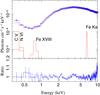 |
Fig. 7 Average spectrum data (blue circles) with uncertainties (crosses) and fitted model (Eq. (1), red line). |
In Fig. 6 we present the variation of some parameters with time. The upper panel shows the evolution of the absorption. Although TBabs is not devised to provide the absorption of X-ray radiation through ionised stellar winds, we use it here as a gauge to qualitatively estimate the changes in the absorbing column. The first absorption column stays constant at around ~ 0.5 × 1022 cm2, which is compatible with the ISM value deduced from the optical data (0.8 × 1022 cm2, using the E(B − V) of Table 1). In turn, the second absorption component represents the absorption of the ISM plus the circum-source environment, presumably the stellar wind. It is high at the beginning of the observation, coinciding with the suppression of the second peak in the light curve at low energies. Then it steadily decreases until the end of the observation. The partial covering fraction C, a proxy for the wind-clumping factor, is very low in general, compared to other sources with supergiant donors, which are always close to 1. It is lower in the beginning of the observation, when the absorption is higher. These values are consistent with those found by (Pradhan et al. 2015) using Suzaku. The spectral index α remains constant and <1, indicating an efficient Comptonising process (see Table A.1). The radius of the source emitting the seed soft photons, which are subsequently Comptonised, can be estimated assuming that the source is radiating as a blackbody of area  (Torrejón et al. 2004),
![Mathematical equation: \begin{equation} R_{W}=0.6\sqrt{L_{34}}(kT)^{-2}~[\rm km], \label{ec:solucion} \end{equation}](/articles/aa/full_html/2017/10/aa30119-16/aa30119-16-eq96.png) (2)where L34 is the luminosity of the bmc component in units of 1034 erg/s and kT is the temperature of the seed soft photons. In Table 4 we list the corresponding radii. The values are low (~ 1.5 − 3.5 km), which is only compatible with a hot spot over a NS surface.
(2)where L34 is the luminosity of the bmc component in units of 1034 erg/s and kT is the temperature of the seed soft photons. In Table 4 we list the corresponding radii. The values are low (~ 1.5 − 3.5 km), which is only compatible with a hot spot over a NS surface.
Luminosity and radii of the seed soft photon source.
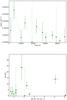 |
Fig. 8 Variation of the Fe Kα emission line. The upper panel shows the line flux versus time. The Fe line is weaker in the second half of the observation. In the lower panel, we plot the variation of the equivalent width (EW) versus the density column of the absorbing material. It does not show the linear trend that is expected when the reprocessing material is spherically distributed around the X-ray source (Torrejón et al. 2010; Giménez-García et al. 2015). |
3.3. RGS spectrum
We present the first high-resolution spectra ever obtained for this source using the XMM-Newton RGS spectrometer in Fig. 9. The continuum was modelled following the EPIC analysis presented before. The spectral parameter α and the temperature kT were fixed to the best-fit values obtained above7, while the normalization and absorption were left free to vary.
The emission lines were fitted with Gaussians. In agreement with the EPIC analysis, two broad emission features at 0.38 keV (C v Lyα) and 0.42 keV (N vi) are clearly detected. When modelled using single Gaussians, they are very broad (σ ~ 1 keV), suggesting a complex structure. The N vi He-like triplet was modelled, thus, with three Gaussians representing the resonant (r), intercombination (i), and forbidden (f) transitions. The widths were fixed to σ = 50 eV. The parameter G = (f + i) /r = 4.1 was found to be consistent with a photoionised plasma at kTe ~ 106 K, while the parameter R = f/i = 0.56 indicates electron plasma densities of ne ~ 1011 cm-3 (Porquet & Dubau 2000). The C v line is blended with a transition at 0.39 keV that is compatible with S xiv, whose emissivity peaks at 3.2 × 10⁶ K. These lines dominate the spectrum at low energies. Aditional emission lines can be seen at 0.681 keV (O vii Lyα), 0.746 keV (Fe xvii), and 0.791 keV (Fe xviii), although with a much lower intensity.
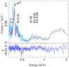 |
Fig. 9 Time-averaged RGS spectrum data (blue) and model (red). |
4. Discussion
The supergiant stellar wind. Several emission lines are detected in the EPIC and RGS spectra. These lines are excited by the intense X-ray irradiation of the donor’s wind. The strongest line is the Fe Kα fluorescence line at 6.4 keV. However, the strength of this line (EWmax ≈ 24 eV) is much weaker than that seen in other HMXBs with supergiant companions (Giménez-García et al. 2015),(Torrejón et al. 2010). There are several possible explanations for this fact: a) the illuminated wind could have a much lower density; b) the wind material could be mostly ionised; or c) the wind could be under-abundant in Fe. Explanations b) and c) seem unlikely. A high ionisation of the wind material contradicts the fact that the photoelectric absorption of local origin is not negligible. An under-abundance of Fe is not expected at all in a system that underwent an SN explosion in the past. Explanation a) is also problematic. In a long-term study of the optical spectra, Reig et al. (2016) found a strong Hα emission that sometimes shows a P Cygni profile. The donor star therefore has a substantial wind (Ṁ ~ 10-6 − 10-7M⊙ yr-1).
The weakness of the Fe Kα fluorescence line might be related to the low covering fraction C. This would indicate a clumping factor much lower than those observed in other supergiant systems. In order to have a strong Fe Kα line, the ionisation parameter  , where n(rX) is the local particle density and rX is the distance from the X-ray source (the NS), must be ≤ 102. In this case, ξ ≥ 102, which means that for an LX ~ 1036 erg s-1 and the characteristic distances within the system rX ~ 1011 − 12 cm, the wind densities should be n ~ 1010 − 12 cm-3. Wind densities like this are a factor 1 to 100 above the smooth wind density predictions. In other words, Fe Kα is mostly produced in the wind clumps. Therefore, 4U 0114+65 seems to have the typical thick wind of a supergiant star, but with a much lower degree of clumping. The donor in 4U 0114+65 (B1Ia) is the coolest of the supergiant X-ray binaries (Krtička et al. 2015). With a Teff = 24 kK, 4U 0114+65 is in the middle of the bistability jump (see low panel in Fig. 3 presented by Vink et al. 1999). This jump is caused by the sudden change in the ionisation balance of Fe (iii, iv), which is a major contributor to the acceleration of the wind. We suggest that this could have a strong impact on the efficiency of the mechanism to form and/or destroy clumps.
The light curve displays narrow (short) and wide (long) dips within the HF states (Fig. 5). In the narrow dips the colour ratio tends to increase, which indicates increased absorption as the most probable cause. On the other hand, in the wide dips the colour ratio tends to remain constant. Thus, the origin of the dips must be related to a general decrease in the mass accretion rate. A straightforward interpretation of the dips would indentify them with wind clumps (short dips) and the interclump medium (long dips). In order to estimate their characteristic sizes, we multiplied the time duration by vrel (Table 1). The long dip size is ≃ 1.6 × 10-3R∗ (4 ± 3 × 109 cm), while the short dip size is ≃ 1.2 × 10-2R∗ (2.9 ± 2.2 × 1010 cm). Interestingly, the ratio long over short is ≃ 7, which is close to the interclump to clump size ratio expected from theoretical models (Martínez-Núñez et al. 2017).
The nature of the X-ray pulsations. The data presented in this study support the interpretation of slow X-ray pulsations seen in the X-ray light curve of 4U 0114+65 in terms of the spin of accreting strongly magnetised NS. As we showed, the spectra of 4U 0114+65 can be described by Comptonisation models. The high temperature of the emitting plasma and the modest luminosity displayed by the source (LX ~ 1036 erg s-1) indicate a small emitting area (of the order of 3 km), compatible with a hot spot over the NS surface. Moreover, the secular spin period decrease observed along the years is not explained in the structured wind scenario presented by Koenigsberger et al. (2006). We therefore conclude that the most likely origin of the pulse is the spin of the NS.
The observed properties of 4U 0114+65 can be explained in the frame of the theory of quasi-spherical settling accretion onto slowly rotating magnetised neutron stars elaborated by Shakura et al. (2012) and further developed in Shakura et al. (2014; see Shakura et al. 2015 and Shakura & Postnov 2017 for a review of the theory and applications). This regime of accretion from a stellar wind can be realised in sources with moderate X-ray luminosity (below ≃ 4 × 1036 erg s-1). In this regime, a hot convective quasi-spherical shell is formed above the NS magnetosphere, and the plasma entry rate from the shell through the magnetosphere is regulated by the cooling of the hot plasma (due to Compton and radiative energy losses). The hot shell mediates the angular momentum transfer to and from the rotating NS. The equilibrium spin period of NS (at which torques acting on the NS magnetosphere on average vanish) in such a case is mostly determined by the velocity of the stellar wind captured by the NS at the Bondi radius RB (vrel in Table 1), the orbital binary period Pb, and the neutron star magnetic field (conveniently expressed in terms of the dipole angular momentum  , where B0 is the neutron star surface magnetic field, RNS is the neutron star radius),
 ![Mathematical equation: \begin{equation} P_{\rm eq}\approx 1000~[{\rm s}] \mu_{30}^{12/11} \left(\frac{P_{\rm b}}{10\,\mathrm{d}}\right)\dot M_{16}^{-4/11}v_8^4 \label{e:Peq} \end{equation}](/articles/aa/full_html/2017/10/aa30119-16/aa30119-16-eq162.png) (3)where μ30 ≡ μ/ (1030 G cm3) and Ṁ16 ≡ Ṁ/ (1016 g s-1), v8 ≡ vrel/ (1000 km s-1). The stellar wind velocity in 4U 0114+65 is about v8 ~ 0.5 − 0.7 (Table 1). For the observed pulse period, Eq. (3) implies a high NS magnetic field, of the order of μ30 ~ 100, that is, in the magnetar range. This does not seem exotic at present (see e.g. recent indications on the magnetar nature of a slowly rotating neutron star in the supernova remnant RCW103, Rea et al. 2016; D’Aì et al. 2016).
(3)where μ30 ≡ μ/ (1030 G cm3) and Ṁ16 ≡ Ṁ/ (1016 g s-1), v8 ≡ vrel/ (1000 km s-1). The stellar wind velocity in 4U 0114+65 is about v8 ~ 0.5 − 0.7 (Table 1). For the observed pulse period, Eq. (3) implies a high NS magnetic field, of the order of μ30 ~ 100, that is, in the magnetar range. This does not seem exotic at present (see e.g. recent indications on the magnetar nature of a slowly rotating neutron star in the supernova remnant RCW103, Rea et al. 2016; D’Aì et al. 2016).
In the case of such a strong magnetic field, the Alfvén radius of the magnetosphere NS is ![Mathematical equation: \begin{equation} R_{\rm A}\approx 1.4\times 10^9~[\mathrm{cm}]\mu_{30}^{6/11}\dot M_{16}^{-2/11}\sim 1.7\times 10^{10}~[\mathrm{cm}] \label{e:RA} \end{equation}](/articles/aa/full_html/2017/10/aa30119-16/aa30119-16-eq168.png) (4)which is still much smaller than the corotation radius Rc = (GMNS/ω2)1 / 3 ~ 7 × 1010 cm. This secures a persistent accretion regime onto the slowly rotating NS even with such a strong magnetic field. The source 4U 0114+65 could then be an accreting magnetar (Reig et al. 2012). This might seem to be at odds with the detection of a cyclotron resonance scattering feature at E ≃ 22 keV (Bonning & Falanga 2005). This detection is uncertain, however, because other studies (Masetti et al. 2005; den Hartog et al. 2006; Wang 2011) have not been able to confirm its existence.
(4)which is still much smaller than the corotation radius Rc = (GMNS/ω2)1 / 3 ~ 7 × 1010 cm. This secures a persistent accretion regime onto the slowly rotating NS even with such a strong magnetic field. The source 4U 0114+65 could then be an accreting magnetar (Reig et al. 2012). This might seem to be at odds with the detection of a cyclotron resonance scattering feature at E ≃ 22 keV (Bonning & Falanga 2005). This detection is uncertain, however, because other studies (Masetti et al. 2005; den Hartog et al. 2006; Wang 2011) have not been able to confirm its existence.
In Fig. 10 we plot the fractional pulse period derivative versus period for magnetars taken from the McGill Magnetar Catalog (Olausen & Kaspi 2014), along with HMXB pulsars taken from the literature. The sources labelled with a C have cyclotron line detections and are therefore not magnetars. The source 4U 0114+65 occupies the same locus as the remaining HMXBs and is close to 4U 2206+54, another wind-accreting magnetar candidate. Both sources are at the top of the period derivative distribution. However, non-magnetar sources such as GX301−2 also occupy this area. There seems to be no clear segregation in this axis. On the other hand, the spin periods of classical magnetars are evidently typically much shorter than the period of X-ray pulsars, including the two accreting magnetar candidates.
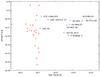 |
Fig. 10 Ṗ/P (s-1) versus P for magnetars (red asterisks; Olausen & Kaspi 2014), HMXBs (blue circles; Ferrigno et al. 2008; Beri & Paul 2017; Barnstedt et al. 2008; Sahiner et al. 2012; Evangelista et al. 2010; Hemphill et al. 2016; Doroshenko et al. 2017; Şahiner et al. 2012), and accreting magnetar candidates (green squares; this work; Wang 2013). The values of Ṗ/P(s-1) are represented in absolute values. Sources labelled with a C present cyclotron lines and are therefore not magnetars. |
Compilation of various spectral model parameters used in the literature to fit X-ray spectra of HMXBs, accreting magnetars (HMXB-AM), and classical magnetars (M).
In an attempt to compare the spectral parameters of different types of sources, we compiled data from the literature in Table 5. Although a meaningful analysis should involve a homogeneous modelling of all sources8, some conclusions can be drawn. The seed photon source temperatures of wind-accreting systems (HMXB, including magnetar candidates) is significantly higher than in classical (non-accreting) magnetars. This might be a consequence of the continuous deposition of energy by the accreted matter in the former. On the other hand, the spectra of accreting systems are harder on average than in classical magnetars. This might be due to a higher efficiency of the Comptonisation mechanism in accreting systems. However, there seems to be no clear difference between accreting magnetar candidates and the other HMXBs.
The nature of the low-luminosity episodes. Two episodes of low X-ray emission were observed during our observations. The first was only seen at low energies and coincided with a period of high absorption. This can be interpreted as a stellar wind structure that momentarily obscures the X-ray source. We can estimate the size of this structure as l ≃ vreltlow, where  is the wind velocity relative to the NS and tlow is the duration of the low-flux episode. From the analysis of the light curve this turns out to be of the order of tlow ~ 24.6 ± 0.2 ks (≲ two pulses). For the relative velocities given in Table 1, this translates into l ~ [ 0.30 − 0.94 ] × 1012 cm ≃[ 0.1 − 0.4 ] R∗. This demonstrates that there are large over-dense structures in the supergiant wind, comparable in size with the stellar radius. Figure 8 shows that the Fe Kα line norm is higher during this first episode of low luminosity than during the remaining observation. This suggests that this large over-dense structure is being momentarily illuminated by the NS X-rays, thereby exciting the Fe fluorescence. The presence of such large structures, likely corotating interaction regions (or CIRs), is commonly invoked to explain the periodic variability observed in the UV spectral lines formed in stellar winds of B-type supergiants (Lobel & Blomme 2008) as well as the modulation of X-ray emission from O stars (Oskinova et al. 2001; Massa et al. 2014).
The interpretation of the second low-luminosity episode is more complex as it affects all energies. Two mechanisms can cause the pronounced flux decrease: either an increased absorption, or a decrease in mass accretion rate. The first mechanism would require an optically thick structure eclipsing the X-ray source. The duration of the eclipse in the current study is tlow ~ 5.4 ± 0.7 ks. Therefore, the structure size would be l ~ [ 0.6 − 2.3 ] × 1011 cm ≃[ 0.02 − 0.09 ] R∗. If the eclipse were caused by an optically thick structure (unless the obscuring structure is also eclipsing the Fe Kα reprocessing region), we would observe an enhancement in the EW of the Fe Kα line as is regularly seen in other HMXBs (Torrejón et al. 2010). This is very unlikely as this region has an extent larger than 1 R∗ (Torrejon et al. 2015).
The second mechanism involves a cessation of the mass accretion onto the NS. This could be accomplished in two ways. The first way would be to encounter a region of very low wind density, a wind bubble (van der Meer et al. 2005). This also would contradict a nearly constant or even slightly increasing absorbing column NH as deduced from the observations. Therefore, a wind bubble seems unlikely. The second mechanism could be centrifugal inhibition of accretion. This propeller mechanism originally suggested by Illarionov & Sunyaev (1975) is now frequently invoked to explain observed low-luminosity episodes in some X-ray pulsars (see e.g. the recent paper of Lutovinov et al. 2017 and references therein). It could also be responsible for many of the off states (periods in which the accretion is totally halted) seen in some HMXBs (cf. Kreykenbohm et al. 2008). However, the NS in 4U 0114+65 has a spin period of 2.6 h, which, as we showed, renders the propeller mechanism ineffective (RA ≪ Rc) even for magnetar fields. For a propeller to start operating, the Alfvèn radius RA should become comparable to the corotation radius Rc. This would require a drop of 1000 times in the X-ray luminosity. An alternative explanation of the observed low-luminosity episode could involve a substantial departure from the spherical accretion symmetry. The Bondi radius is an idealisation and could change by a factor 2 or 3 in different directions, as the stellar wind velocity changes on the characteristic scale of 1011 cm, which is comparable to RB (see Table 1). The stellar wind could then be momentarily captured in a non-spherical way. Since the magnetospheric radius and the Bondi radius differ only by a factor of a few, the captured matter can reach the magnetosphere non-spherically, thereby enabling a switching between the magnetic poles of the NS. This pole switching can also be responsible for the pulse shape change displayed by the source between T1 and T2.
5. Summary and conclusions
We have performed a time-resolved investigation of one of the slowest pulsars ever found using a 49 ks uninterrupted observation with the XMM-Newton. The following conclusions can be drawn from our analysis:
-
1.
We successfully fit the pulse-phase resolved spectra with a bulk motion Comptonisation model (bmc) for the first time. This model implies a very small (r ~ 3 km) and hot (kT ~ 2 − 3 keV) emitting region and therefore points to a hot spot on the surface of a rotating NS as the most likely explanation for the X-ray pulse.
-
2.
The long NS spin period (Pspin ~ 9.4 ks) and the secular spin-up
Hz s-1 can be explained within the theory of quasi-spherical settling accretion onto the NS provided that the magnetic field is in the magnetar range μ30 ~ 30 − 100. -
3.
Owing to the extremely slow NS rotation period, even with such a strong magnetic field, the magnetospheric radius (RA) is still much smaller than the corotation radius Rc. This is consistent with the persistent nature of this source.
-
4.
The stellar wind of the supergiant star presents a covering fraction (~ 0.3) much lower than typically found for other systems with supergiant donors (~ 0.8 − 0.9). This indicates a much lower degree of wind clumping. This is also supported by the much weaker Fe Kα line as compared to other HMXBs. We suggest that the proximity of 4U 0114+65 to the bistability jump, where the mass loss and the wind acceleration change dramatically, could have a strong impact on wind clump formation.
-
5.
The light curve presents dips that are clearly seen within the HF states. The short dips tend to show a colour ratio increase and would be caused by wind clump absorption. The long dips, in turn, tend to show a constant CR and would be produced by a general decrease in the mass accretion rate associated with the pass of an interclump zone by the NS. Its characteristic sizes would be ≃ 1.6 × 10-3R∗ (4 ± 3 × 109 cm) and ≃ 1.2 × 10-2R∗ (2.9 ± 2.2 × 1010 cm) for the long and short dips, respectively. The interclump to clump size ratio observed is ~ 7, which is close to the expected value (~ 10) predicted by the theoretical models of stellar winds in massive stars.
-
6.
We detected two episodes of low luminosity. The first affects only the low energies and can be attributed to a large (l ~ [ 0.3 − 0.5 ] R∗) over-dense structure in the B1 supergiant donor wind, compatible with a corotating interaction region (CIR). The second episode affects all energies. An eclipse due to an optically thick structure or accretion failure caused by a rarefied cavity in the wind seems to be unlikely. Considering the small difference (within a factor of one) between the Bondi and magnetospheric radii, spherically asymmetric capture of matter close to the Bondi radius might cause temporal cessation of accretion onto one NS magnetic pole. Such a mass accretion redistribution between the NS poles could also produce the observed change in the NS pulse shape.
Charge-coupled device.
Maintained by HEASARC at NASA/GSFC.
Even though the source shows a clear spin-up trend, some episodes of torque reversal were detected, each lasting approximatelyone year (see Sood et al. 2006).
Note that the colour ratio is much higher in HS2 than in HF6 because the higher general abosorption during the first part of the observation (see Table A.1).
RGS is not sensitive to these parameters given the narrow energy range considered and its soft response.
The power-law photon index Γ and the BMC spectral index α are not directly comparable. The same is true for the blackbody temperature and the colour temperature of the seed photons. This would require a large-scale reanalysis, which is beyond the scope of this paper.
Acknowledgments
This work has been funded by the research grants ESP2014-53672-C3-3P and 50 OR 1508 (LO). We acknowledge the detailed comments of the anonymous referee that improved the content and presentation of the paper. The authors acknowledge the hospitality of the ISSI in Bern under the team lead by S. Martinez.
References
- Barnstedt, J., Staubert, R., Santangelo, A., et al. 2008, A&A, 486, 293 [NASA ADS] [CrossRef] [EDP Sciences] [Google Scholar]
- Beri, A., & Paul, B. 2017, New Astron., 56, 94 [NASA ADS] [CrossRef] [Google Scholar]
- Bonning, E. W., & Falanga, M. 2005, A&A, 436, L31 [NASA ADS] [CrossRef] [EDP Sciences] [Google Scholar]
- Bozzo, E., Falanga, M., & Stella, L. 2008, ApJ, 683, 1031 [NASA ADS] [CrossRef] [Google Scholar]
- Şahiner, Ş., Inam, S. Ç., & Baykal, A. 2012, MNRAS, 421, 2079 [NASA ADS] [CrossRef] [Google Scholar]
- Crampton, D., Hutchings, J. B., & Cowley, A. P. 1985, ApJ, 299, 839 [NASA ADS] [CrossRef] [Google Scholar]
- D’Aì, A., Evans, P. A., Burrows, D. N., et al. 2016, MNRAS, 463, 2394 [NASA ADS] [CrossRef] [Google Scholar]
- den Hartog, P. R., Hermsen, W., Kuiper, L., et al. 2006, A&A, 451, 587 [NASA ADS] [CrossRef] [EDP Sciences] [Google Scholar]
- Doroshenko, R., Santangelo, A., Doroshenko, V., & Piraino, S. 2017, A&A, 600, A52 [NASA ADS] [CrossRef] [EDP Sciences] [Google Scholar]
- Dower, R., Kelley, R., Margon, B., & Bradt, H. 1977, IAU Circ., 3144 [Google Scholar]
- Duncan, R. C., & Thompson, C. 1992, ApJ, 392, L9 [NASA ADS] [CrossRef] [Google Scholar]
- Evangelista, Y., Feroci, M., Costa, E., et al. 2010, ApJ, 708, 1663 [NASA ADS] [CrossRef] [Google Scholar]
- Farrell, S. A., Sood, R. K., & O’Neill, P. M. 2006, MNRAS, 367, 1457 [NASA ADS] [CrossRef] [Google Scholar]
- Farrell, S. A., Sood, R. K., O’Neill, P. M., & Dieters, S. 2008, MNRAS, 389, 608 [NASA ADS] [CrossRef] [Google Scholar]
- Ferrigno, C., Segreto, A., Mineo, T., Santangelo, A., & Staubert, R. 2008, A&A, 479, 533 [NASA ADS] [CrossRef] [EDP Sciences] [Google Scholar]
- Finley, J. P., Belloni, T., & Cassinelli, J. P. 1992, A&A, 262, L25 [NASA ADS] [Google Scholar]
- Fornasini, F. M., Tomsick, J. A., Bachetti, M., et al. 2017, ApJ, 841, 35 [NASA ADS] [CrossRef] [Google Scholar]
- Fürst, F., Pottschmidt, K., Kreykenbohm, I., et al. 2012, A&A, 547, A2 [NASA ADS] [CrossRef] [EDP Sciences] [Google Scholar]
- Giménez-García, A., Torrejón, J. M., Eikmann, W., et al. 2015, A&A, 576, A108 [NASA ADS] [CrossRef] [EDP Sciences] [Google Scholar]
- Grundstrom, E. D., Blair, J. L., Gies, D. R., et al. 2007, ApJ, 656, 431 [NASA ADS] [CrossRef] [Google Scholar]
- Hall, T. A., Finley, J. P., Corbet, R. H. D., & Thomas, R. C. 2000, ApJ, 536, 450 [NASA ADS] [CrossRef] [Google Scholar]
- Hemphill, P. B., Rothschild, R. E., Fürst, F., et al. 2016, MNRAS, 458, 2745 [NASA ADS] [CrossRef] [Google Scholar]
- Ikhsanov, N. R., & Beskrovnaya, N. G. 2013, Astron. Rep., 57, 287 [NASA ADS] [CrossRef] [Google Scholar]
- Illarionov, A. F., & Sunyaev, R. A. 1975, A&A, 39, 185 [NASA ADS] [Google Scholar]
- Koenigsberger, G., Georgiev, L., Moreno, E., et al. 2006, A&A, 458, 513 [NASA ADS] [CrossRef] [EDP Sciences] [Google Scholar]
- Kreykenbohm, I., Wilms, J., Kretschmar, P., et al. 2008, A&A, 492, 511 [NASA ADS] [CrossRef] [EDP Sciences] [Google Scholar]
- Krtička, J., Kubát, J., & Krtičková, I. 2015, A&A, 579, A111 [NASA ADS] [CrossRef] [EDP Sciences] [Google Scholar]
- Lamers, H. J. G. L. M., & Cassinelli, J. P. 1999, Introduction to Stellar Winds, 452 [Google Scholar]
- Li, X.-D., & van den Heuvel, E. P. J. 1999, ApJ, 513, L45 [NASA ADS] [CrossRef] [Google Scholar]
- Lobel, A., & Blomme, R. 2008, ApJ, 678, 408 [NASA ADS] [CrossRef] [Google Scholar]
- Lomb, N. R. 1976, Ap&SS, 39, 447 [NASA ADS] [CrossRef] [Google Scholar]
- Lutovinov, A. A., Tsygankov, S. S., Krivonos, R. A., Molkov, S. V., & Poutanen, J. 2017, ApJ, 834, 209 [NASA ADS] [CrossRef] [Google Scholar]
- Martínez-Núñez, S., Kretschmar, P., Bozzo, E., et al. 2017, Space Sci. Rev., in press [arXiv:1701.08618] [Google Scholar]
- Masetti, N., Orlandini, M., Dal Fiume, D., et al. 2005, ArXiv e-prints [arXiv:astro-ph/0508451] [Google Scholar]
- Massa, D., Oskinova, L., Fullerton, A. W., et al. 2014, MNRAS, 441, 2173 [NASA ADS] [CrossRef] [Google Scholar]
- Olausen, S. A., & Kaspi, V. M. 2014, ApJS, 212, 6 [NASA ADS] [CrossRef] [Google Scholar]
- Oskinova, L. M., Clarke, D., & Pollock, A. M. T. 2001, A&A, 378, L21 [NASA ADS] [CrossRef] [EDP Sciences] [Google Scholar]
- Porquet, D., & Dubau, J. 2000, A&AS, 143, 495 [NASA ADS] [CrossRef] [EDP Sciences] [Google Scholar]
- Pradhan, P., Paul, B., Paul, B. C., Bozzo, E., & Belloni, T. M. 2015, MNRAS, 454, 4467 [NASA ADS] [CrossRef] [Google Scholar]
- Rea, N., Borghese, A., Esposito, P., et al. 2016, ApJ, 828, L13 [NASA ADS] [CrossRef] [Google Scholar]
- Reig, P., Chakrabarty, D., Coe, M. J., et al. 1996, A&A, 311, 879 [NASA ADS] [Google Scholar]
- Reig, P., Torrejón, J. M., & Blay, P. 2012, MNRAS, 425, 595 [NASA ADS] [CrossRef] [Google Scholar]
- Reig, P., Nersesian, A., Zezas, A., Gkouvelis, L., & Coe, M. J. 2016, A&A, 590, A122 [NASA ADS] [CrossRef] [EDP Sciences] [Google Scholar]
- Roberts, D. H., Lehar, J., & Dreher, J. W. 1987, AJ, 93, 968 [NASA ADS] [CrossRef] [Google Scholar]
- Sahiner, S., Inam, S. C., Baykal, A., & Kiziloglu, U. 2012, ArXiv e-prints [arXiv:1212.3433] [Google Scholar]
- Scargle, J. D. 1982, ApJ, 263, 835 [NASA ADS] [CrossRef] [Google Scholar]
- Shakura, N., & Postnov, K. 2017, ArXiv e-prints [arXiv:1702.03393] [Google Scholar]
- Shakura, N., Postnov, K., Kochetkova, A., & Hjalmarsdotter, L. 2012, MNRAS, 420, 216 [NASA ADS] [CrossRef] [Google Scholar]
- Shakura, N. I., Postnov, K. A., Kochetkova, A. Y., & Hjalmarsdotter, L. 2014, EPJ Web Conf., 64, 02001 [Google Scholar]
- Shakura, N. I., Postnov, K. A., Kochetkova, A. Y., et al. 2015, Astron. Rep., 59, 645 [NASA ADS] [CrossRef] [Google Scholar]
- Sidoli, L., Tiengo, A., Paizis, A., et al. 2017, ApJ, 838, 133 [NASA ADS] [CrossRef] [Google Scholar]
- Sood, R., Farrell, S., O’Neill, P., Manchanda, R., & Ashok, N. M. 2006, Adv. Space Res., 38, 2779 [NASA ADS] [CrossRef] [Google Scholar]
- Strüder, L., Briel, U., Dennerl, K., et al. 2001, A&A, 365, L18 [NASA ADS] [CrossRef] [EDP Sciences] [Google Scholar]
- Titarchuk, L., Mastichiadis, A., & Kylafis, N. D. 1997, ApJ, 487, 834 [NASA ADS] [CrossRef] [Google Scholar]
- Torrejón, J. M., Kreykenbohm, I., Orr, A., Titarchuk, L., & Negueruela, I. 2004, A&A, 423, 301 [NASA ADS] [CrossRef] [EDP Sciences] [Google Scholar]
- Torrejón, J. M., Schulz, N. S., Nowak, M. A., & Kallman, T. R. 2010, ApJ, 715, 947 [NASA ADS] [CrossRef] [Google Scholar]
- van der Meer, A., Kaper, L., di Salvo, T., et al. 2005, A&A, 432, 999 [NASA ADS] [CrossRef] [EDP Sciences] [Google Scholar]
- Vink, J. S., de Koter, A., & Lamers, H. J. G. L. M. 1999, A&A, 350, 181 [NASA ADS] [Google Scholar]
- Wang, W. 2011, MNRAS, 413, 1083 [NASA ADS] [CrossRef] [Google Scholar]
- Wang, W. 2013, MNRAS, 432, 954 [NASA ADS] [CrossRef] [Google Scholar]
- Wilms, J., Allen, A., & McCray, R. 2000, ApJ, 542, 914 [NASA ADS] [CrossRef] [Google Scholar]
Appendix A: Phase-resolved spectra for the bmc model
Phase-resolved parameters for the spectral model.
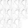 |
Fig. A.1 Spectra for the BMC model. The panels are in chronological order. |
Appendix B: Phase-resolved analysis of the emission line parameters
Phase-resolved analysis of the emission lines.
All Tables
Velocity of the stellar wind, calculated with a β-law equation: , with the value β = 0.8 (Lamers & Cassinelli 1999), at the site of the NS.
Compilation of various spectral model parameters used in the literature to fit X-ray spectra of HMXBs, accreting magnetars (HMXB-AM), and classical magnetars (M).
All Figures
|
Fig. 1 Sketch of the system where we can compare the size of the donor star with the orbit (NS size not to scale). The light curve is displayed parallel to the orbit. |
| In the text | |
|
Fig. 2 Light curve in two different energy ranges: upper panel 0.3–3.0 keV, and middle panel 3–10 keV. The lower panel shows the colour ratio (3–10) keV/(0.3–3.0) keV. The vertical green line divides T1 and T2 time intervals. The labels LF5a and LF5b refer to low-flux intervals, see text for detail. The epoch time corresponds to 57 255.50 MJD. |
| In the text | |
|
Fig. 3 Evolution of the pulse frequency from 1986 to 2015. |
| In the text | |
|
Fig. 4 0.3–10 keV light curve, folded on the spin period (9320 ± 1 s), for T1 (blue solid line) and T2 (green dashed line). The epoch time is 57 255.50 MJD. |
| In the text | |
|
Fig. 5 Detailed view of two light curve sections, HF2 (top panel) and HF6 (bottom panel). Each panel is additionally subdivided into three divisions. The upper division corresponds to the low-energy light curve, the middle division to the high-energy light curve, and the lower division to the colour ratio. The short and long dips are marked by green and magenta lines, respectively. |
| In the text | |
|
Fig. 6 Evolution of the density columns (top) and radius of the seed soft photon source (bottom) for the bmc model. The top panel shows that the first-component absorption (red line) remains constant, compatible wih the ISM medium. The blue line represents the absorption of the ISM plus the circum-source environment, which changes during the observation. It is particularly high at the beginning of the observation, when the low-energy light curve is partially suppressed. |
| In the text | |
|
Fig. 7 Average spectrum data (blue circles) with uncertainties (crosses) and fitted model (Eq. (1), red line). |
| In the text | |
|
Fig. 8 Variation of the Fe Kα emission line. The upper panel shows the line flux versus time. The Fe line is weaker in the second half of the observation. In the lower panel, we plot the variation of the equivalent width (EW) versus the density column of the absorbing material. It does not show the linear trend that is expected when the reprocessing material is spherically distributed around the X-ray source (Torrejón et al. 2010; Giménez-García et al. 2015). |
| In the text | |
|
Fig. 9 Time-averaged RGS spectrum data (blue) and model (red). |
| In the text | |
|
Fig. 10 Ṗ/P (s-1) versus P for magnetars (red asterisks; Olausen & Kaspi 2014), HMXBs (blue circles; Ferrigno et al. 2008; Beri & Paul 2017; Barnstedt et al. 2008; Sahiner et al. 2012; Evangelista et al. 2010; Hemphill et al. 2016; Doroshenko et al. 2017; Şahiner et al. 2012), and accreting magnetar candidates (green squares; this work; Wang 2013). The values of Ṗ/P(s-1) are represented in absolute values. Sources labelled with a C present cyclotron lines and are therefore not magnetars. |
| In the text | |
|
Fig. A.1 Spectra for the BMC model. The panels are in chronological order. |
| In the text | |
Current usage metrics show cumulative count of Article Views (full-text article views including HTML views, PDF and ePub downloads, according to the available data) and Abstracts Views on Vision4Press platform.
Data correspond to usage on the plateform after 2015. The current usage metrics is available 48-96 hours after online publication and is updated daily on week days.
Initial download of the metrics may take a while.