| Issue |
A&A
Volume 605, September 2017
|
|
|---|---|---|
| Article Number | A40 | |
| Number of page(s) | 10 | |
| Section | Stellar structure and evolution | |
| DOI | https://doi.org/10.1051/0004-6361/201730654 | |
| Published online | 06 September 2017 | |
WHT follow-up observations of extremely metal-poor stars identified from SDSS and LAMOST⋆
1 Instituto de Astrofísica de Canarias, Vía Láctea, 38205 La Laguna, Tenerife, Spain
e-mail: This email address is being protected from spambots. You need JavaScript enabled to view it.
2 Universidad de La Laguna, Departamento de Astrofísica, 38206 La Laguna, Tenerife, Spain
3 Consejo Superior de Investigaciones Científicas, 28006 Madrid, Spain
Received: 17 February 2017
Accepted: 25 May 2017
Abstract
Aims. We have identified several tens of extremely metal-poor star candidates from SDSS and LAMOST, which we follow up with the 4.2 m William Herschel Telescope (WHT) telescope to confirm their metallicity.
Methods. We followed a robust two-step methodology. We first analyzed the SDSS and LAMOST spectra. A first set of stellar parameters was derived from these spectra with the FERRE code, taking advantage of the continuum shape to determine the atmospheric parameters, in particular, the effective temperature. Second, we selected interesting targets for follow-up observations, some of them with very low-quality SDSS or LAMOST data. We then obtained and analyzed higher-quality medium-resolution spectra obtained with the Intermediate dispersion Spectrograph and Imaging System (ISIS) on the WHT to arrive at a second more reliable set of atmospheric parameters. This allowed us to derive the metallicity with accuracy, and we confirm the extremely metal-poor nature in most cases. In this second step we also employed FERRE, but we took a running mean to normalize both the observed and the synthetic spectra, and therefore the final parameters do not rely on having an accurate flux calibration or continuum placement. We have analyzed with the same tools and following the same procedure six well-known metal-poor stars, five of them at [Fe/H] <−4 to verify our results. This showed that our methodology is able to derive accurate metallicity determinations down to [Fe/H] <−5.0.
Results. The results for these six reference stars give us confidence on the metallicity scale for the rest of the sample. In addition, we present 12 new extremely metal-poor candidates: 2 stars at [Fe/H] ≃−4, 6 more in the range −4 < [Fe / H] < −3.5, and 4 more at −3.5 < [Fe / H] < −3.0.
Conclusions. We conclude that we can reliably determine metallicities for extremely metal-poor stars with a precision of 0.2 dex from medium-resolution spectroscopy with our improved methodology. This provides a highly effective way of verifying candidates from lower quality data. Our model spectra and the details of the fitting algorithm are made public to facilitate the standardization of the analysis of spectra from the same or similar instruments.
Key words: stars: abundances / stars: fundamental parameters / stars: Population II / galaxies: stellar content / Galaxy: halo
The model spectra are only available at the CDS via anonymous ftp to cdsarc.u-strasbg.fr (130.79.128.5) or via http://cdsarc.u-strasbg.fr/viz-bin/qcat?J/A+A/605/A40
© ESO, 2017
1. Introduction
The oldest stars in the Galactic halo contain information about the early Universe after the primordial nucleosynthesis. These stars are key for understanding how galaxies form, what the masses of the first generation of stars were, and what the early chemical evolution of the Milky Way was like. The oldest stars are extremely poor in heavy elements and havemost likely been preceded locally by only one massive Population III star (Frebel et al. 2015). Chemical abundances in extremely metal-poor (EMP) stars (with [Fe / H] < −3), in particular dwarf EMP stars, are needed to study the difference between the primordial lithium abundance obtained from standard Big Bang nucleosynthesis, constrained by the baryonic density inferred from the Wilkinson Microwave Anisotropy Probe (WMAP) observations of the Cosmic microwave background (CMB; Spergel et al. 2003), and in situ atmospheric abundance measurements from old metal-poor turn-off stars (Spite & Spite 1982; Rebolo et al. 1988; González Hernández et al. 2008; Bonifacio et al. 2009; Sbordone et al. 2012). Unfortunately, very metal-poor stars are extremely rare, with fewer than ten stars known in the [Fe / H] < −4.5 regime. This seriously limits the number of lithium measurements and detections that are required to shed light on this problem.
Coordinates and atmospheric parameters for the program stars based in the analysis of the low-resolution spectra with FERRE.
Detailed chemical abundance determinations of EMP stars require high-resolution spectroscopy (e.g. Roederer et al. 2014; Frebel & Norris 2015), but the identification of these stars is a difficult task. In the 1980’s and 1990’s several different techniques were designed and applied to search for metal-poor stars of the Galactic halo using various telescopes that were equipped with low- and medium-resolution spectrographs (Beers et al. 1985, 1992; Ryan & Norris 1991; Carney et al. 1996). More recently, the stars with the lowest iron abundances have been discovered from candidates identified in the Hamburg-ESO survey (Christlieb et al. 2002) or the Sloan Digital Sky Survey (SDSS York et al. 2000; Bonifacio et al. 2012). In the past decade, additional stars have been identified by photometric surveys such as the one using the SkyMapper Telescope, see Keller et al. (2012), or the Pristine Survey (Starkenburg et al. 2017), and spectroscopic surveys such as the Radial Velocity Experiment (RAVE, Fulbright et al. 2010), the Sloan Extension for Galactic Understanding and Exploration (SEGUE, Yanny et al. 2009), or the large Sky Area Multi-Object Fiber Spectroscopic Telescope (LAMOST, Deng et al. 2012). Extremely metal-poor stars tend to be located at large distances. For these stars, spectroscopic surveys usually do not provide spectra with sufficient quality, and it is therefore critical to examine and verify candidates with additional observations with higher quality.
In this work, we follow a two-step methodology to identify new extremely metal-poor stars: we perform an improved analysis of SDSS and LAMOST data to select EMP candidates, and we carry out follow-up observations of a subsample, which allows us to check the stellar parameters, metallicities, and carbon abundances of these candidates. The paper is organized as follows. In Sect. 2 we explain the candidate selection. Section 3 is devoted to the follow-up observations and data reduction. Section 4 describes in detail how the analysis was carried out, including tests using well-known metal-poor stars (Sect. 4.1). We then discuss our carbon abundance determination from low- and medium-resolution spectra (Sect. 4.3). Finally, Sect. 5 summarizes our results and conclusions.
2. Low spectral resolution analysis and target selection
We have analyzed the low-resolution spectra of more than 2.5 million targets from three different surveys: the Baryonic Oscillations Spectroscopic Survey (BOSS, Eisenstein et al. 2011; Dawson et al. 2013), SEGUE (Yanny et al. 2009), and LAMOST (Deng et al. 2012). The analysis of the stars from these surveys was performed with FERRE1 (Allende Prieto et al. 2006), which allowed us to derive the main stellar parameters, effective temperature Teff, and surface gravity log g, together with the metallicity [Fe/H]2 and carbon abundance [C/Fe] (see Aguado et al. 2016, for further details). As a result of the extremely low metal abundances of our targets, iron transitions are not detected, either individually or even as blended features, in medium-resolution spectra. We typically measured only the Ca ii resonance lines and used them as a proxy for the overall metal abundance of the stars, assuming the typical iron-to-calcium ratio found in metal-poor stars, [Fe/H] = [ Ca / H ] −0.4.
We analyzed about 1 700 000 (~1 500 000 stars) spectra from LAMOST, 740 000 (~660 000 stars) from SEGUE and 340 000 (~300 000 stars) from BOSS. A database with all candidates at [ Fe / H ] < −3.5 was built that contains ~500 objects with a first set of stellar properties (Teff, log g, [Fe/H], and [C/Fe]). However, this first selection still contains many outliers and unreliable fits. We reevaluated the goodness of fit by measuring the χ2 in a limited spectral region around the Balmer lines. This method prevents false positives even at low signal-to-noise ratios (S/N< 20). Finally, a visual inspection of the spectra and their best fittings was carried out to select, to skim the best several tens of candidates. The stars that passed this selection were then scheduled for observations at medium-resolution and much higher S/N. Table 1 shows the derived parameters of the final sample that was analyzed in this work. Visual inspection helps us to detect promising candidates. The two LAMOST objects discussed below are good example for cases where visual inspection was critical. In addition to these stars, we chose some of the most metal-poor stars known ([ Fe / H ] < −4.0), with published determinations from high-resolution spectroscopic data, in order to test our methodology.
3. Observations and data reduction
The second step in our methodology makes use of follow-up medium-resolution spectroscopy obtained with the Intermediate dispersion Spectrograph and Imaging System (ISIS) (Jorden 1990) spectrograph on the 4.2 m William Herschel Telescope (WHT) at the Observatorio del Roque de los Muchachos (La Palma, Spain). We used the R600B and R600R gratings, the GG495 filter in the red arm, and the default dichroic (5300 Å). The mean FWHM resolution with a one-arcsecond slit was R ~ 2400 in the blue arm and R ~ 5200 in the red arm. More details are provided in Aguado et al. (2016). The observations were carried out over the course of five observing runs: run I: Dec. 31−Jan. 2, 2015 (three nights); run II: February 5−8, 2015 (four nights); run III: August 14−18, 2015 (five nights); run IV: May 1−2, 2016 (two nights), and run V: July 29−31, 2016 (three nights). A standard data reduction (bias substraction, flat-fielding and wavelength calibration, using CuNe + CuAr lamps) was performed with the onespec package in IRAF3 (Tody 1993).
High-resolution spectra of well-known metal-poor stars were extracted from the ESO archive4 and obtained with the Ultraviolet and Visual Echelle Spectrograph (UVES, Dekker et al. 2000) at the VLT. The spectral range of these data is 3300−4500 Å and the resolving power is about 47 000. The spectra were reduced using the automatic UVES pipeline (Ballester et al. 2000), offered to the community through the ESO Science Archive Facility.
4. Analysis and discussion
In order to derive the stellar parameters and chemical abundances a grid of synthetic spectra was computed with the ASSϵT code (Koesterke et al. 2008), which uses the Barklem codes (Barklem et al. 2000a,b) to describe the broadening of the Balmer lines. This grid resembles the grid used by Allende Prieto et al. (2014), with some differences described below, and it is provided ready to be used with FERRE as an electronic table. The model atmospheres were computed with the same Kurucz codes and strategies as described by Mészáros et al. (2012). The abundance of α-elements was fixed to [ α/ Fe ] = + 0.4, and the limits of the grid were −6 ≤ [ Fe / H ] ≤ −2; −1 ≤ [ C / Fe ] ≤ 5, 4750 K ≤ Teff ≤ 7000 K and 1.0 ≤ log g ≤ 5.0, assuming a microturbulence of 2 km s-1. We searched for the best fit using FERRE by simultaneously deriving the main three atmospheric parameters and the carbon abundance.
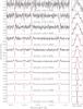 |
Fig. 1 Left panel: medium-resolution ISIS spectrum of G64-12 with different levels of added Poisson noise (black lines) and the best fit computed with FERRE (red line). Right panel: Gaussian distribution of the S/N computed on the residuals from subtracting the best-fitting model from the observed spectrum. |
Stellar parameters and main results obtained from ISIS spectra.
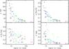 |
Fig. 2 Random errors derived with FERRE as a function of the S/N for individual and combined exposures. Each color represents a different star. The triangles correspond to the combined spectra, and asterisks indicate the individual exposures, with random errors estimated with FERRE and given in Table 2. The squares show the dispersion in the parameters derived from individual exposures, shown at the mean value of their S/N. |
Interstellar reddening and the instrument response distort the intrinsic shape of the stellar spectra. To minimize systematic differences between the synthetic spectra and the observations, we worked with continuum-normalized fluxes. The observed and synthetic spectra were both normalized using a running-mean filter with a width of 30 pixels (about 10 Å). Although the precision in the derived parameters was found to be very sensitive to the normalization scheme, our tests showed that when no reliable information on the shape spectral energy distribution is available, the running-mean filter offers very good performance. With this modification we were able to retrieve Teff and log g information from ISIS spectra.
In order to determine how robust the FERRE results are, we carried out a series of consistency tests by adding random noise with a normal distribution to an observed spectrum of the metal-poor star G64-12. The results are illustrated in Fig. 1 and are described below. We find that FERRE is able to recover the original set of parameters from high S/N values down to S/N = 15 when the derived solution begins to drift away from the expected solution. This is consistent with the results obtained by Allende Prieto et al. (2014) for SDSS spectroscopy.
We used observations of well-known metal-poor stars to test our methodology. The comparison between the literature metallicities from high-resolution analyses and those we obtained using medium-resolution spectroscopy indicates that our approach works quite well. Nonetheless, our methodology does not allow us to separate the Ca ii K spectral lines from the star from the interstellar medium (ISM) contributions that are not resolved in the ISIS spectra. Below, we describe tests in which we reanalyzde the original UVES spectra (see Sect. 4.1) of several objects after smoothing to understand the effect of having a lower spectral resolution.
FERRE is able to derive internal uncertainties in several ways. After extensive testing in our ISIS spectra, we find that the best option is to inject noise using a normal distribution to the observed spectra several times, and search for the best-fitting parameters. Such Monte Carlo simulations were performed 50 times for each observed spectrum. The dispersion in the derived parameters was adopted as a measurement of the internal uncertainty on these parameters in our analysis. In addition to the final combined spectra for each target, we analyzed each individual exposure in the same way. Figure 2 shows the relationship between our derived internal random uncertainties and the S/N. The uncertainties on the final combined spectra follow the same trend as was found in the analysis of individual exposures. The only giant star in the sample, J2045+1508, shows a higher uncertainty in its surface gravity determination, as expected (see Table 2). From these tests, we conclude that our random errors are consistently and reliably determined, with the exception of the [C/Fe] abundance ratios, for which we tend to underestimate the random uncertainties, given that the dispersion from individual estimates of this parameter is larger than the random error from individual exposures. This is particularly relevant at [C/Fe] < 1.0 dex.
In addition to random errors, other sources of systematic uncertainty can affect our results. Stellar effective temperatures are not easy to determine accurately (see, e.g., Sbordone et al. 2010). We adopted a 100 K uncertainty following the comparison between photometric and spectroscopic methods by Yong et al. (2004). In addition, the stellar isochrones depicted in Fig. 7 suggest that systematic 0.3−0.5 dex error could be present in our spectroscopic gravities (see Sects. 4.2 and 5). Based on these comparisons, we decided to adopt a systematic uncertainty in surface gravity of 0.5 dex. The error bars shown for the data in Fig. 7 are the quadratic combination of our estimated random and systematic uncertainties. We adopted a 0.1 dex metallicity error, according to the comparisons between our results and those in the high-resolution analyses in the literature, but we caution that much larger systematic uncertainties could be present as a result of departures from local thermal equilibrium (LTE) and hydrostatic equilibrium (see Shchukina et al. 2005; Nordlander et al. 2017, and references therein), which could add up to 0.8−0.9 dex. Based on other works (see Sect. 4.3) we estimate that our derived carbon abundances could have a systematic uncertainty of about 0.3 dex. In Table 3 we show the carbon abundances for well-known metal-poor stars whose uncertainties were computed by adding in quadrature the random error and the adopted systematic error.
4.1. Well-known metal-poor stars
4.1.1. G64-12
Aoki et al. (2006) observed G64-12 with the High Dispersion Spectrograph (HDS) at the Subaru telescope and derived its main atmospheric parameters as Teff = 6390 ± 100 K, log g = 4.4 ± 0.3, and [Fe / H] = −3.2 ± 0.1. We obtained with ISIS at the WHT a high-quality spectrum (S/N ~ 300) of this object and derived a set of parameters that excellently agree with those from Aoki et al. (2006): Teff = 6377 ± 104 K, log g = 4.8 ± 0.7, and [Fe / H] = −3.2 ± 0.2.
4.1.2. SDSS J1313−0019
There is an open debate about the metallicity of this object, discovered by Allende Prieto et al. (2015) using a low-resolution spectrum from the BOSS project (Eisenstein et al. 2011; Dawson et al. 2013). Allende Prieto et al. (2015) derived the following set of parameters: Teff = 5300 ± 50 K, log g = 3.0 ± 0.2, [Fe / H] = −4.3 ± 0.1, and [C / Fe] = 2.5 ± 0.1. This temperature reproduces both the local continuum slope and the shape of the Balmer lines in the BOSS spectrum of the star. Shortly after the discovery, Frebel et al. (2015) obtained a high-resolution (R ~ 35 000) spectrum with the MIKE spectrograph at the Magellan-Clay telescope. Their adopted effective temperature and surface gravity are Teff = 5200 ± 150 K and log g = 2.6 ± 0.7. They measured 37 Fe i lines (Fe ii features were not detected) and estimated a metallicity of [Fe / H] = −5.00 ± 0.28 and [C / Fe] = 2.96 ± 0.28.
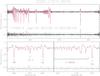 |
Fig. 3 Top panel: blue ISIS J1313−0019 spectrum (black line) and the best fit computed with FERRE (red line) with the residuals (black line over blue reference). The derived stellar parameters and carbon abundance are shown. Bottom panel: detail of the Ca ii H-K and the g-band spectral region. |
Carbon abundance results.
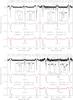 |
Fig. 4 Spectra in the range of the Ca ii lines for four well-known metal-poor stars. From top to bottom: UVES, UVES smoothed to ISIS resolution, ISIS spectra (black line), and the best medium-resolution fit (red line). Details of the calcium lines in the UVES spectra are included in the insets together with the effective temperature and metallicity derived with FERRE for UVES-smoothed and ISIS spectra. |
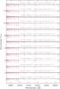 |
Fig. 5 ISIS/WHT blue arm spectra (3700 Å–4900 Å) for the full sample (black line) and the best fit calculated with FERRE (red line). The main stellar parameters are also displayed. |
A high-S/N medium-resolution spectrum of J1313−0019 was obtained as part of our WHT program. Figure 3 shows the entire spectrum and the best-fitting spectrum from the FERRE analysis. We derive Teff = 5525 ± 106 K, log g = 3.6 ± 0.5, [Fe / H] = −4.7 ± 0.2, and [C / Fe] = 2.8 ± 0.30. Our derived metallicity is in between those by Allende Prieto et al. (2015) and Frebel et al. (2015), but closer to the determination by Frebel et al. (2015). When we use carbon-enhanced model atmospheres, consistent with the high [C/Fe] ratio adopted in the spectral synthesis, it does not introduce significant changes in the derived values. The difference between our analysis and that in Allende Prieto et al. (2015) is partly explained by the fact that we assume [ α/ H ] = 0.4, while the authors derived [ α/ H ] = 0.2 ± 0.1.
We checked that when we impose in the FERRE analysis the same effective temperature and surface gravity as adopted by Frebel et al. (2015) (Teff = 5200 and log g = 2.6), we recover a metallicity and carbon abundance of [Fe / H] = −4.9 ± 0.2 and [C / Fe] = 2.7 ± 0.3, respectively. The adoption of an effective temperature 300 K cooler by Frebel et al. (2015) is responsible for an offset of about 0.2 dex in metallicity. Since our value of Teff (see Table 2) is mostly based on fitting all the Balmer lines available in the spectrum we consider it reliable.
4.1.3. HE 0233−0343
This star was studied by Hansen et al. (2014) using high-resolution spectra acquired with UVES on the VLT, and it is one of the rare stars at such a low metallicity where the lithium abundance was measured, A(Li) = 1.77. These objects are key for understanding the cosmological Li problem (e.g. Asplund et al. 2006; Bonifacio et al. 2007; González Hernández et al. 2008). Our effective temperature determination, Teff = 6150 ± 103 K, is consistent with the temperature proposed by Hansen et al. (2014) of Teff = 6100 ± 100 K. They assumed an age of 10 Gyr to infer a surface gravity of log g = 3.4 ± 0.3 from isochrones, while we derive log g = 4.9 ± 0.7 from the ISIS spectrum.
Calcium ISM absorption is clearly visible in the UVES spectrum of this star, but it is not resolved at the ISIS resolution (see Fig. 4). An unresolved ISM contribution biases our metallicity determination from FERRE to [Fe / H] = −4.0 ± 0.1, while Hansen et al. (2014) derived [Fe / H] = −4.7 ± 0.2. To check the consistency of the high- and medium-resolution results, we smoothed the UVES spectrum to the ISIS resolution and reanalyzed it. We arrived at the same result as for the ISIS data: Teff = 6207 K; log g = 4.9, and [Fe / H] = −4.0, as illustrated in Fig. 4.
4.1.4. SDSS J1029+1729
The star SDSS J1029+1729 has no carbon (or nitrogen) detected, which makes it the most metal-poor star ever discovered (Caffau et al. 2011, 2012). This rare object challenges theoretical calculations that predict that no low-mass stars can form at very low metallicities. Using UVES with a resolving power R ~ 38 000, (Caffau et al. 2012) derived the following set of parameters: Teff = 5811 ± 150 K, log g = 4.0 ± 0.5, and [Fe / H] = −4.9 ± 0.2. Our analysis of the medium-resolution ISIS spectra arrives at Teff = 5845 ± 105 K, log g = 5.0 ± 0.8 and [Fe / H] = −4.4 ± 0.2. Following a similar argument as given in Sect. 4.1.3, the difference in metallicity is associated with the calcium ISM contribution (See Fig. 4). This is demonstrated by degrading the UVES spectrum to the resolution of the ISIS data. This analysis gives a result that is fully consistent with the result from the ISIS spectrum: Teff = 5867 K, log g = 5.0, and [Fe / H] = −4.5.
4.1.5. HE 1327−2326
The study of this star is complicated because of the complex structure of the calcium ISM features and the extraordinary amount of carbon ([ C / Fe ] = 4.26, Frebel et al. 2005; Aoki et al. 2006) in the stellar atmosphere (see Fig. 4). The parameters from Aoki et al. (2006) from a high-resolution UVES spectrum are Teff = 6180 ± 100 K, log g = 3.7 ± 0.3, and [Fe / H] = −5.6 ± 0.1 while FERRE returns Teff = 6150 ± 102 K, log g = 4.3 ± 0.7, and [Fe / H] = −4.8 ± 0.2 from the medium-resolution ISIS spectrum. We display in Fig. 4 the original UVES observation, the same data smoothed to the resolution of ISIS, and the ISIS spectrum.
The UVES spectrum resolves multiple ISM features, while ISIS only uncovers some of the blue components so that the FERRE analysis of the ISIS spectrum returns a higher metallicity. The smoothed spectrum solution is again consistent with our own medium-resolution ISIS values: Teff = 6119 K; log g = 4.3, and [Fe / H] = −4.9. The use of medium-resolution data inevitably leads to a biased metallicity because of the unresolved ISM calcium absorption.
4.1.6. SDSS J1442−0015
The S/N of this spectrum is the lowest in our sample since it is one of the faintest metal-poor star in the [Fe / H] < −4.0 regime. Even so, the original set parameters derived from UVES spectroscopy by Caffau et al. (2013), Teff = 5850 ± 150 K, log g = 4.0 ± 0.5, and [Fe / H] = −4.1 ± 0.2, are in fair agreement with our determinations from ISIS data: Teff = 6036 ± 102 K, log g = 4.9 ± 0.5, and [Fe / H] = −4.4 ± 0.2.
The spectrum of J1442−0015 clearly shows an ISM contribution to the observed calcium absorption, but this component is already resolved in the ISIS data (see Fig. 4). The effective temperature adopted by Caffau et al. (2013), which is slightly lower than our FERRE estimate, should lead to a difference of at least ~0.4 dex between the two metallicity determinations but in the opposite direction to what we find. In addition, our analysis of the UVES spectrum smoothed to the resolution of ISIS provides a Teff = 6167 K, log g = 4.9 and [Fe / H] = −4.2, consistent with the results from ISIS.
4.2. New set of extremely metal-poor stars
Following the same methodology as in Sect. 4.1, we analyzed spectra from the ISIS instrument for a sample of metal-poor star candidates identified from SDSS and LAMOST. The mean S/N of these spectra is around 75, so we expect the FERRE results to be reliable. Our effective temperatures are trustworthy, since we were able to recover the temperature for several well-known metal-poor stars whose metallicities are consistent with the literature values. In addition, the derived metallicities by FERRE are also reliable and consistent with the results obtained from the analysis of SDSS spectra (see Allende Prieto et al. 2014, for further details). Only our surface gravities appear to be subject to a systematic error of about 0.5 dex. This is in contrast to the small random uncertainties we derive for our stellar parameters, and to the surface gravity in particular (Sect. 4): lower than 0.1 dex at S/N ~ 50.
Figure 7 shows DARMOUTH isochrones5, HB, and AGB tracks compared to the stellar parameters derived using FERRE on the ISIS spectra and their derived error bars. Our mean uncertainty in the metallicity determination is 0.12 dex, whereas the mean uncertainty in Teff is 103 K.
The mean metallicity difference between our first metallicity estimates from SDSS/LAMOST spectra and the second estimate we obtain from higher quality ISIS spectra is 0.31 dex with a standard deviation of 0.20 dex. In this computation we excluded the stars J134157+513534 and J132917+542027, since the metallicity differences for them are much larger. The LAMOST spectra of these stars show several artifacts that do not allow us to perform a correct continuum normalization with our running-mean algorithm, and consequently, we cannot derive reliable parameters from these data. However, our ISIS spectra have significantly higher quality, S/N ~ 82 and 76, and we finally derived a reliable metallicity for both stars, [Fe/H] =−2.7 and [Fe/H] =−3.5, respectively. In Fig. 6 we compare the results that are summarized in Table 2 with those from the low-resolution analysis (Table 1). In addition, we reanalyzed the stars studied in Aguado et al. (2016) with the improved methodology we presented here. We obtain a slightly higher dispersion for candidates with lower quality spectra.
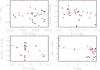 |
Fig. 6 Comparison between the main stellar parameters derived with FERRE from low-resolution (SDSS and LAMOST) data and from ISIS spectra. Objects included in our sample appear as black filled stars while objects from our previous work Aguado et al. (2016) are red filled stars. |
Our analysis uncovers two objects (J0304+3910 and J1055+2322) at [Fe/H] ≃−4.0 and six more at −3.5 ≥ [Fe/H] >−4.0, in the domain of the extremely metal-poor stars, and most of them appear to be dwarfs at log g ≥ 4.0. A deeper study of this sample using high-resolution spectroscopy would provide abundances for additional elements, which would help to constrain the nature of the stars and the early chemical evolution of the Galaxy.
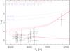 |
Fig. 7 DARMOUTH isochrones for [Fe / H] = −3.5 and different ages from 16 to 10 Gyr (red dashed lines), and blue dashed lines are the HB and AGB theoretical tracks for [Fe / H] = −2.5 for two different relative masses (M = 0.6 and M = 1.0). The black diamonds represent the stars of this work and their internal uncertainties derived with the FERRE code. |
4.3. Carbon abundances
Carbon-enhanced metal-poor (CEMP) stars are defined by Beers & Christlieb (2005) as stars with [C/Fe] ≥ + 1.0. The fraction of CEMP/EMP stars increases as metallicity decreases. Deriving reliable carbon abundances in metal-poor stars using medium-resolution spectroscopy is not always possible (Bonifacio et al. 2015). For the well-known EMP sample studied in Sect. 4.1, we recover carbon abundances that are compatible with the literature values for three CEMP stars: SDSS J1313−0019, HE 1327−2326, and HE 0233−0343 (see Table 3).
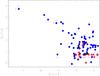 |
Fig. 8 Carbon over iron versus metallicities of stars presented in this work (black filled stars) and those from Aguado et al. (2016, red filled stars) analyzed with the improved methodology, together with stars from the literature (Sivarani et al. 2006; Yong et al. 2013; Frebel et al. 2005, 2006; Caffau et al. 2014; Allende Prieto et al. 2015) represented by blue filled circles. |
Figure 8 shows the carbon abundances derived from ISIS spectra for the targets studied in this work, together with those from Aguado et al. (2016), with the improved methodology, and other CEMP stars from the literature. The data suggest that the lower the metallicity, the stronger the carbon enhancement, as expected (see, e.g., Lee et al. 2013). Our ability to measure carbon abundances decreases as the effective temperature of the star increases because of CH dissociation. Empirically, to measure carbon abundances at the level of [C/Fe] ≥ + 0.5, the star should have Teff ~ 5500 / 5700 K. Moreover, if the effective temperature lies at ~5000 / 5100 K, we are able to measure carbon at [C/Fe] ≥ + 0.0. In addition, an S/N of at least 30 is required to derive reliable carbon abundances. Table 2 summarizes our results and shows that our sample includes at least three confirmed CEMP stars: SDSS J0151+1639, SDSS J1733+3329, and SDSS J2310+1210 with [Fe/H] =−3.8, −3.4, and −3.8, respectively, in perfect agreement with the statistics by Cohen & Huang (2009), Bonifacio et al. (2015). In addition, five more stars appear to be very close to our detection limit of [C/Fe] ~ + 0.7−0.8.
5. Conclusions
We have demonstrated that our methodology for identifying metal-poor stars using low- and medium-resolution spectroscopy is effective. We were able to scrutinize more than 2.5 million spectra from SDSS and LAMOST to identify extremely metal-poor star candidates, which we followed up with significantly higher S/N and slightly higher resolution ISIS observations. Our success in identifying metal-poor candidates is quite high, with only one star, J1329+5420, at [Fe/H] >−3.
The use of the FERRE code and a custom grid of synthetic spectra allowed us to simultaneously derive the atmospheric parameters and the carbon abundance, which improved our values from SDSS or LAMOST. We showed that FERRE can be used efficiently on extremely metal-poor stars. We make our tools publicly available to facilitate the cross-calibration of results from other teams. Our method offers an excellent way to identify and analyze CEMP star candidates without the need for high-resolution spectroscopy. We presented a new EMP sample and reliable determinations of the metallicities and carbon abundances of these stars.
These stars, especially the two at [Fe/H] <−4.0, are good candidates for follow-up high-resolution observations. This domain is sparsely populated, with fewer than 30 known stars, and it is of high interest for investigating the early chemical evolution of the Galaxy. The fact that we have used a grid of synthetic spectra including carbon as a free parameter not only in the synthesis but in the model atmospheres helps us to detect promising extremely metal-poor stellar candidates and derive their carbon abundances when [C/Fe] > 0.7−1.0 and S/N> 30 / 40, and even lower carbon enhancements and/or S/N values if the star is colder than 5500 K.
We included in our work several well-known metal-poor stars that were previously analyzed in the literature. A study of these objects is useful to check for systematic differences that are due to multiple analysis methods. Our results shown that we are able to recover the effective temperature with an uncertainty of about 100 K and the metallicity within 0.2 dex. In addition, the comparison of our parameters with model isochrones suggests that our surface gravities have a systematic uncertainty of about 0.5 dex. Our study also confirms that we are able to recover the carbon abundance for CEMP stars using medium-resolution spectra.
Future work should include observations at higher resolution of the most interesting extremely metal-poor stars identified in this paper to study their chemical abundance patterns in detail.
FERRE is available from http://github.com/callendeprieto/ferre
We use the bracket notation to report chemical abundances: [a/b]  , where N(x) represents number the density of nuclei of the element x.
IRAF is distributed by the National Optical Astronomy Observatory, which is operated by the Association of Universities for Research in Astronomy (AURA) under cooperative agreement with the National Science Foundation.
Based on data from the ESO Science Archive Facility.
The Dartmouth Stellar Evolution Program (DSEP) is available from www.stellar.dartmouth.edu
Acknowledgments
D.A. is thankful to the Spanish Ministry of Economy and Competitiveness (MINECO) for financial support received in the form of a Severo-Ochoa PhD fellowship, within the Severo-Ochoa International PhD Program. D.A., C.A.P., J.I.G.H., and R.R. acknowledge the Spanish ministry project MINECO AYA2014-56359-P. J.I.G.H. acknowledges financial support from the Spanish Ministry of Economy and Competitiveness (MINECO) under the 2013 Ramón y Cajal program MINECO RYC-2013-14875. This paper is based on observations made with the William Herschel Telescope, operated by the Isaac Newton Group at the Observatorio del Roque de los Muchachos, La Palma, Spain, of the Instituto de Astrofísica de Canarias. We thank the ING staff members for their assistance and efficiency during the four observing runs in visitor mode. The author gratefully acknowledges the technical expertise and assistance provided by the Spanish Supercomputing Network (Red Espanola de Supercomputacion), as well as the computer resources used: the LaPalma Supercomputer, located at the Instituto de Astrofisica de Canarias.
References
- Aguado, D. S., Allende Prieto, C., González Hernández, J. I., et al. 2016, A&A, 593, A10 [NASA ADS] [CrossRef] [EDP Sciences] [Google Scholar]
- Allende Prieto, C., Beers, T. C., Wilhelm, R., et al. 2006, ApJ, 636, 804 [NASA ADS] [CrossRef] [Google Scholar]
- Allende Prieto, C., Fernández-Alvar, E., Schlesinger, K. J., et al. 2014, A&A, 568, A7 [NASA ADS] [CrossRef] [EDP Sciences] [Google Scholar]
- Allende Prieto, C., Fernández-Alvar, E., Aguado, D. S., et al. 2015, A&A, 579, A98 [NASA ADS] [CrossRef] [EDP Sciences] [Google Scholar]
- Aoki, W., Frebel, A., Christlieb, N., et al. 2006, ApJ, 639, 897 [NASA ADS] [CrossRef] [Google Scholar]
- Asplund, M., Lambert, D. L., Nissen, P. E., Primas, F., & Smith, V. V. 2006, ApJ, 644, 229 [NASA ADS] [CrossRef] [Google Scholar]
- Ballester, P., Modigliani, A., Boitquin, O., et al. 2000, The Messenger, 101, 31 [NASA ADS] [Google Scholar]
- Barklem, P. S., Piskunov, N., & O’Mara, B. J. 2000a, A&AS, 142, 467 [NASA ADS] [CrossRef] [EDP Sciences] [MathSciNet] [PubMed] [Google Scholar]
- Barklem, P. S., Piskunov, N., & O’Mara, B. J. 2000b, A&A, 363, 1091 [NASA ADS] [Google Scholar]
- Beers, T. C., & Christlieb, N. 2005, in Highlights of Astronomy, 13, 579 [NASA ADS] [Google Scholar]
- Beers, T. C., Preston, G. W., & Shectman, S. A. 1985, AJ, 90, 2089 [NASA ADS] [CrossRef] [Google Scholar]
- Beers, T. C., Preston, G. W., & Shectman, S. A. 1992, AJ, 103, 1987 [NASA ADS] [CrossRef] [Google Scholar]
- Bonifacio, P., Molaro, P., Sivarani, T., et al. 2007, A&A, 462, 851 [NASA ADS] [CrossRef] [EDP Sciences] [Google Scholar]
- Bonifacio, P., Spite, M., Cayrel, R., et al. 2009, A&A, 501, 519 [NASA ADS] [CrossRef] [EDP Sciences] [Google Scholar]
- Bonifacio, P., Sbordone, L., Caffau, E., et al. 2012, A&A, 542, A87 [NASA ADS] [CrossRef] [EDP Sciences] [Google Scholar]
- Bonifacio, P., Caffau, E., Spite, M., et al. 2015, A&A, 579, A28 [NASA ADS] [CrossRef] [EDP Sciences] [Google Scholar]
- Caffau, E., Bonifacio, P., François, P., et al. 2011, Nature, 477, 67 [NASA ADS] [CrossRef] [PubMed] [Google Scholar]
- Caffau, E., Bonifacio, P., François, P., et al. 2012, A&A, 542, A51 [NASA ADS] [CrossRef] [EDP Sciences] [Google Scholar]
- Caffau, E., Bonifacio, P., François, P., et al. 2013, A&A, 560, A15 [NASA ADS] [CrossRef] [EDP Sciences] [Google Scholar]
- Caffau, E., Sbordone, L., Bonifacio, P., et al. 2014, Mem. Soc. Astron. Ital., 85, 222 [Google Scholar]
- Carney, B. W., Laird, J. B., Latham, D. W., & Aguilar, L. A. 1996, AJ, 112, 668 [NASA ADS] [CrossRef] [Google Scholar]
- Christlieb, N., Wisotzki, L., & Graßhoff, G. 2002, A&A, 391, 397 [NASA ADS] [CrossRef] [EDP Sciences] [Google Scholar]
- Cohen, J. G., & Huang, W. 2009, ApJ, 701, 1053 [NASA ADS] [CrossRef] [Google Scholar]
- Dawson, K. S., Schlegel, D. J., Ahn, C. P., et al. 2013, AJ, 145, 10 [Google Scholar]
- Dekker, H., D’Odorico, S., Kaufer, A., Delabre, B., & Kotzlowski, H. 2000, in Optical and IR Telescope Instrumentation and Detectors, eds. M. Iye, & A. F. Moorwood, Proc. SPIE, 4008, 534 [Google Scholar]
- Deng, L.-C., Newberg, H. J., Liu, C., et al. 2012, Res. Astron. Astrophys., 12, 735 [NASA ADS] [CrossRef] [Google Scholar]
- Eisenstein, D. J., Weinberg, D. H., Agol, E., et al. 2011, AJ, 142, 72 [Google Scholar]
- Frebel, A., & Norris, J. E. 2015, ARA&A, 53, 631 [NASA ADS] [CrossRef] [Google Scholar]
- Frebel, A., Aoki, W., Christlieb, N., et al. 2005, Nature, 434, 871 [NASA ADS] [CrossRef] [PubMed] [Google Scholar]
- Frebel, A., Christlieb, N., Norris, J. E., et al. 2006, ApJ, 652, 1585 [NASA ADS] [CrossRef] [Google Scholar]
- Frebel, A., Chiti, A., Ji, A. P., Jacobson, H. R., & Placco, V. M. 2015, ApJ, 810, L27 [NASA ADS] [CrossRef] [Google Scholar]
- Fulbright, J. P., Wyse, R. F. G., Ruchti, G. R., et al. 2010, ApJ, 724, L104 [NASA ADS] [CrossRef] [Google Scholar]
- González Hernández, J. I., Caballero, J. A., Rebolo, R., et al. 2008, A&A, 490, 1135 [NASA ADS] [CrossRef] [EDP Sciences] [Google Scholar]
- Hansen, T., Hansen, C. J., Christlieb, N., et al. 2014, ApJ, 787, 162 [NASA ADS] [CrossRef] [Google Scholar]
- Jorden, P. R. 1990, in Instrumentation in Astronomy VII, ed. D. L. Crawford, SPIE Conf. Ser., 1235, 790 [Google Scholar]
- Keller, S. C., Skymapper Team, & Aegis Team. 2012, in Galactic Archaeology: Near-Field Cosmology and the Formation of the Milky Way, eds. W. Aoki, M. Ishigaki, T. Suda, T. Tsujimoto, & N. Arimoto, ASP Conf. Ser., 458, 409 [Google Scholar]
- Koesterke, L., Allende Prieto, C., & Lambert, D. L. 2008, ApJ, 680, 764 [NASA ADS] [CrossRef] [Google Scholar]
- Lee, Y. S., Beers, T. C., Masseron, T., et al. 2013, AJ, 146, 132 [NASA ADS] [CrossRef] [Google Scholar]
- Mészáros, S., Allende Prieto, C., Edvardsson, B., et al. 2012, AJ, 144, 120 [NASA ADS] [CrossRef] [Google Scholar]
- Nordlander, T., Amarsi, A. M., Lind, K., et al. 2017, A&A, 597, A6 [NASA ADS] [CrossRef] [EDP Sciences] [Google Scholar]
- Rebolo, R., Beckman, J. E., & Molaro, P. 1988, A&A, 192, 192 [NASA ADS] [Google Scholar]
- Roederer, I. U., Preston, G. W., Thompson, I. B., et al. 2014, AJ, 147, 136 [NASA ADS] [CrossRef] [Google Scholar]
- Ryan, S. G., & Norris, J. E. 1991, AJ, 101, 1835 [NASA ADS] [CrossRef] [Google Scholar]
- Sbordone, L., Bonifacio, P., Caffau, E., et al. 2010, A&A, 522, A26 [NASA ADS] [CrossRef] [EDP Sciences] [Google Scholar]
- Sbordone, L., Bonifacio, P., & Caffau, E. 2012, Mem. Soc. Astron. Ital. Suppl., 22, 29 [NASA ADS] [Google Scholar]
- Shchukina, N. G., Trujillo Bueno, J., & Asplund, M. 2005, ApJ, 618, 939 [NASA ADS] [CrossRef] [Google Scholar]
- Sivarani, T., Beers, T. C., Bonifacio, P., et al. 2006, A&A, 459, 125 [NASA ADS] [CrossRef] [EDP Sciences] [Google Scholar]
- Spergel, D. N., Verde, L., Peiris, H. V., et al. 2003, ApJS, 148, 175 [NASA ADS] [CrossRef] [Google Scholar]
- Spite, M., & Spite, F. 1982, Nature, 297, 483 [NASA ADS] [CrossRef] [Google Scholar]
- Starkenburg, E., Martin, N., Youakim, K., et al. 2017, MNRAS, 471, 2587 [NASA ADS] [CrossRef] [Google Scholar]
- Tody, D. 1993, in Astronomical Data Analysis Software and Systems II, eds. R. J. Hanisch, R. J. V. Brissenden, & J. Barnes, ASP Conf. Ser., 52, 173 [Google Scholar]
- Yanny, B., Rockosi, C., Newberg, H. J., et al. 2009, AJ, 137, 4377 [NASA ADS] [CrossRef] [Google Scholar]
- Yong, D., Lambert, D. L., Allende Prieto, C., & Paulson, D. B. 2004, ApJ, 603, 697 [NASA ADS] [CrossRef] [Google Scholar]
- Yong, D., Norris, J. E., Bessell, M. S., et al. 2013, ApJ, 762, 26 [NASA ADS] [CrossRef] [Google Scholar]
- York, D. G., Adelman, J., Anderson, Jr., J. E., et al. 2000, AJ, 120, 1579 [CrossRef] [Google Scholar]
All Tables
Coordinates and atmospheric parameters for the program stars based in the analysis of the low-resolution spectra with FERRE.
All Figures
|
Fig. 1 Left panel: medium-resolution ISIS spectrum of G64-12 with different levels of added Poisson noise (black lines) and the best fit computed with FERRE (red line). Right panel: Gaussian distribution of the S/N computed on the residuals from subtracting the best-fitting model from the observed spectrum. |
| In the text | |
|
Fig. 2 Random errors derived with FERRE as a function of the S/N for individual and combined exposures. Each color represents a different star. The triangles correspond to the combined spectra, and asterisks indicate the individual exposures, with random errors estimated with FERRE and given in Table 2. The squares show the dispersion in the parameters derived from individual exposures, shown at the mean value of their S/N. |
| In the text | |
|
Fig. 3 Top panel: blue ISIS J1313−0019 spectrum (black line) and the best fit computed with FERRE (red line) with the residuals (black line over blue reference). The derived stellar parameters and carbon abundance are shown. Bottom panel: detail of the Ca ii H-K and the g-band spectral region. |
| In the text | |
|
Fig. 4 Spectra in the range of the Ca ii lines for four well-known metal-poor stars. From top to bottom: UVES, UVES smoothed to ISIS resolution, ISIS spectra (black line), and the best medium-resolution fit (red line). Details of the calcium lines in the UVES spectra are included in the insets together with the effective temperature and metallicity derived with FERRE for UVES-smoothed and ISIS spectra. |
| In the text | |
|
Fig. 5 ISIS/WHT blue arm spectra (3700 Å–4900 Å) for the full sample (black line) and the best fit calculated with FERRE (red line). The main stellar parameters are also displayed. |
| In the text | |
|
Fig. 6 Comparison between the main stellar parameters derived with FERRE from low-resolution (SDSS and LAMOST) data and from ISIS spectra. Objects included in our sample appear as black filled stars while objects from our previous work Aguado et al. (2016) are red filled stars. |
| In the text | |
|
Fig. 7 DARMOUTH isochrones for [Fe / H] = −3.5 and different ages from 16 to 10 Gyr (red dashed lines), and blue dashed lines are the HB and AGB theoretical tracks for [Fe / H] = −2.5 for two different relative masses (M = 0.6 and M = 1.0). The black diamonds represent the stars of this work and their internal uncertainties derived with the FERRE code. |
| In the text | |
|
Fig. 8 Carbon over iron versus metallicities of stars presented in this work (black filled stars) and those from Aguado et al. (2016, red filled stars) analyzed with the improved methodology, together with stars from the literature (Sivarani et al. 2006; Yong et al. 2013; Frebel et al. 2005, 2006; Caffau et al. 2014; Allende Prieto et al. 2015) represented by blue filled circles. |
| In the text | |
Current usage metrics show cumulative count of Article Views (full-text article views including HTML views, PDF and ePub downloads, according to the available data) and Abstracts Views on Vision4Press platform.
Data correspond to usage on the plateform after 2015. The current usage metrics is available 48-96 hours after online publication and is updated daily on week days.
Initial download of the metrics may take a while.