| Issue |
A&A
Volume 604, August 2017
|
|
|---|---|---|
| Article Number | A126 | |
| Number of page(s) | 9 | |
| Section | The Sun | |
| DOI | https://doi.org/10.1051/0004-6361/201730798 | |
| Published online | 25 August 2017 | |
Helioseismic holography of simulated sunspots: dependence of the travel time on magnetic field strength and Wilson depression
1 Instituto de Astrofísica de Canarias, C/vía Láctea, s/n, 38205 La Laguna, Tenerife, Spain
e-mail; This email address is being protected from spambots. You need JavaScript enabled to view it.
2 Departamento de Astrofísica, Universidad de La Laguna, 38205 La Laguna, Tenerife, Spain
3 North West Research Associates, Boulder, CO 80301, USA
4 Max-Planck-Institut für Sonnensystemforschung, Justus-von-Liebig-Weg 3, 37077 Göttingen, Germany
Received: 16 March 2017
Accepted: 25 May 2017
Abstract
Improving methods for determining the subsurface structure of sunspots from their seismic signature requires a better understanding of the interaction of waves with magnetic field concentrations. We aim to quantify the impact of changes in the internal structure of sunspots on local helioseismic signals. We have numerically simulated the propagation of a stochastic wave field through sunspot models with different properties, accounting for changes in the Wilson depression between 250 and 550 km and in the photospheric umbral magnetic field between 1500 and 3500 G. The results show that travel-time shifts at frequencies above approximately 3.50 mHz (depending on the phase-speed filter) are insensitive to the magnetic field strength. The travel time of these waves is determined exclusively by the Wilson depression and sound-speed perturbation. The travel time of waves with lower frequencies is affected by the direct effect of the magnetic field, although photospheric field strengths below 1500 G do not leave a significant trace on the travel-time measurements. These results could potentially be used to develop simplified travel-time inversion methods.
Key words: Sun: helioseismology / Sun: oscillations / sunspots / methods: numerical / Sun: interior / Sun: magnetic fields
© ESO, 2017
1. Introduction
Solar active regions, such as sunspots, are the most remarkable manifestations of solar magnetism and have a key role in the coupling between the interior and the atmosphere, which makes the understanding of sunspot formation, stability, and decay one of the outstanding problems in solar physics. Local helioseismic studies have been focused on solar active regions for more than two decades, but significant uncertainty still exists regarding their interpretation due to the complexity of wave interactions with magnetic fields.
Several helioseismic techniques have been developed to probe the subsurface structure of active regions. The most commonly used measurement is the phase change of waves traveling through the active region, usually described as a change in travel time, which can be obtained from time-distance helioseismology (Duvall et al. 1993), Fourier-Hankel analysis (Braun et al. 1992), or helioseismic holography (Braun & Birch 2008). The first attempts to interpret the seismic signals assumed that sunspots could be characterized as small perturbations to the thermal structure of a quiet Sun model and neglected the direct effects of the magnetic field on helioseismic waves. From this approach two different sunspot scenarios were inferred from observations: a shallow positive perturbation of the sound speed (Fan et al. 1995) and a two-layer model with a reduction of the wave-speed in the top layer and an increase in the wave-speed down to 10 Mm below the surface (Kosovichev 1996; Kosovichev et al. 2000).
Subsequent observational (Lindsey & Braun 2005; Schunker et al. 2005; Couvidat & Rajaguru 2007) and numerical (Cameron et al. 2008; Cally 2009; Moradi et al. 2009; Cameron et al. 2011; Moradi et al. 2015) studies have shown that surface magnetic fields strongly alter travel times. In addition to the changes in the phase speed of the waves introduced by the magnetic field, mode conversion (Schunker & Cally 2006; Cally & Goossens 2008) can also affect the photospheric seismic measurements through the returning of atmospheric fast waves (Rosenthal et al. 2002; Khomenko & Collados 2006; Felipe et al. 2010) or Alfvén waves (Cally & Hansen 2011; Hansen & Cally 2012; Khomenko & Cally 2012; Felipe 2012). Cally & Moradi (2013) quantified the contribution of these returned waves to the travel-time shifts obtained from the analysis of the photospheric wave field. They found a significant travel-time shift that depends on the propagation direction of the waves and the magnetic field inclination.
Recently, Felipe et al. (2016) evaluated the individual contributions of the direct and indirect magnetic effects on the travel-time perturbations measured using helioseismic holography. The term “direct magnetic effects” refers to the changes in wave propagation due to the wave interaction with the magnetic field through mode conversion and fast wave refraction, which produces variations in the wave speed and ray paths. The “indirect magnetic effects” account for the changes in the thermal structure of the sunspot imposed by the presence of the magnetic field. Their results show that waves filtered for certain phase speeds and frequencies are less sensitive to the magnetic field. For those combinations of filters, the travel-time shifts are accurately predicted from the thermal structure of the sunspot, accounting for the Wilson depression and the changes in the sound speed but neglecting the direct effect of the magnetic field. In this work, we aim to further explore the dependence of the helioseismic signals on sunspot properties by analyzing a larger sample of sunspot models that differ in their magnetic field strength and Wilson depression. The numerical methods are described in Sect. 2and the comparison of the results obtained for different models is presented in Sect. 3. Finally, the conclusions and the potential applications of our results are discussed in Sect. 4.
2. Numerical procedures
We carried out twelve numerical simulations of wave propagation through magnetohydrostatic (MHS) sunspot models using the code MANCHA (Khomenko & Collados 2006; Felipe et al. 2010). The numerical setup of all the simulations is the same as described in Felipe et al. (2016). Here we include only a brief description of the numerical configuration. We address the interested reader to Felipe et al. (2016) for a detailed discussion of the numerical methods. The vertical computational domain spans from z = − 25 Mmto z = 1 Mm, with z = 0 defined at the quiet-Sun photosphere and a uniform vertical grid size of 50 km. The dimension of the horizontal directions is 102.4 Mm and they are sampled with a resolution of 200 km. The axes of the sunspots are located at the middle of the domain. The Alfvén speed has been artificially limited to 80 km s-1following Rempel et al. (2009).
The simulations differ in the properties of the MHS models used as background. All the sunspot models were constructed with the same method (Khomenko & Collados 2008), but changing two of their properties: magnetic field strength and Wilson depression. The method combines a self-similar solution (Low 1980) in the deep layers with a current-distributed solution (Pizzo 1986) in the upper layers. This class of models allows the freedom to select the values of several parameters that control the properties of the resultant sunspot model. The magnetic configuration is given by the parameters  , η, and a. The former produces changes in the magnetic field strength, while the magnetic field inclination, the curvature of the field lines, and the radius of the structure depend on the other two parameters. The model used as a boundary condition at the axis of the sunspot can be shifted up or down on the axis in order to account for the Wilson depression zWD. The last parameter that can be modified is the height z0 where the self-similar and current-distributed solutions are merged. The space of parameters explored includes umbral photospheric field strengths of Bu = 1500, 2500, and 3500 G and Wilson depressions of zWD = 250, 350, 450, and 550 km. All the possible combinations of these two parameters were computed, producing a total of twelve independent simulations. The parameters η, a, and z0 are the same for all the models. The radial variation of the photospheric vertical magnetic field approximately follows a Gaussian distribution with a FWHM of 19 Mm (a Gaussian is set at the height z0, but it is modified through an iterative process to concatenate the self-similar and current-distributed models and obtain a MHS solution). The use of models with different magnetic field strength but otherwise the same field geometry allow us to evaluate the effect of field strength on the seismic signal independently of the magnetic field inclination. Figure 1 shows the vertical stratification of the isothermal cut-off frequency for all the models at the center of the sunspot. As expected, an increase in the Wilson depression increases the depth of the upper turning point. In the following, we refer to the “upper turning point” as the depth where the wave frequency is equal to the local cut-off frequency, that is, to the upper turning point of the radial mode. The depth of the
  layer, where c is the sound speed and vA is the Alfvén speed, increases with the magnetic field. This layer is located at a similar depth for all the models with Bu = 3500 G, but for lower field strengths the depth of the β = 1 layer depends on the Wilson depression. Figure 2 illustrates the sound speed. Models with the same Wilson depression but different field strengths present differences in their sound speed, since their gas pressure stratifications differ due to the pressure deficit imposed by the magnetic field.
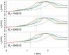 |
Fig. 1 Vertical stratification of the isothermal cut-off frequency at the axis of the sunspot models with Bu = 1500 G (top panel), Bu = 2500 G (middle panel), and Bu = 3500 G (bottom panel), where z is height and z = 0 is defined at the quiet-Sun photosphere. The colored lines correspond to the Wilson depression of the model: zWD = 250 km (black), zWD = 350 km (blue), zWD = 450 km (green), and zWD = 550 km (red). The vertical dotted lines illustrate the height where β = 1 for the model with the Wilson depression associated to the corresponding color. The horizontal thin dashed lines mark some selected frequencies (3.25, 4.25, 5.25 mHz). The thick black dashed line illustrates the cut-off frequency at the quiet-Sun. |
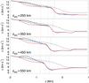 |
Fig. 2 Vertical stratification of the sound speed at the axis of the sunspot models with zWD = 250 km (top panel), zWD = 350 km (second panel), zWD = 450 km (third panel), and zWD = 550 km (bottom panel), where z is height and z = 0 is defined at the quiet-Sun photosphere. The color of the lines indicates the photospheric umbral magnetic field strength of the model: Bu = 1500 G km (black), Bu = 2500 G (blue), and Bu = 3500 G km (red). The vertical dotted lines illustrate the height where β = 1 for the model with the magnetic field associated to the corresponding color. The thick black dashed line illustrates the sound speed in the quiet Sun. |
A quiet Sun simulation with the same setup of the sunspot cases was performed for applying the method of noise subtraction (Werne et al. 2004). Waves are excited by sources introduced in the equations. They are located at 150 kmbelow the photosphere in quiet-Sun regions and their depth increases toward the axis of the spot following a constant temperature surface from the simulation with Bu = 2500 Gand zWD = 450 km. Wave sources are randomly distributed in the horizontal directions, but all the simulations use the same random distribution. As a result, the same quiet-Sun simulation can be used for applying noise subtraction to all the sunspot cases. The duration of the simulations with Bu = 1500 Gand Bu = 2500 Gis 8 h, while the simulations with Bu = 3500 Gspan 7 h of solar time.
Travel times are computed by applying the procedures for surface-focused helioseismic holography (see Braun & Birch 2008) to the vertical velocity maps at constant optical depth τ = 0.01. Filtering has been applied in k − ω space following many previous studies (e.g., Duvall et al. 1997; Kosovichev et al. 2000; Zhao et al. 2001; Braun & Birch 2006; Birch et al. 2009). We use a set of phase-speed filters described in Couvidat et al. (2006). Their mean phase speed spans from 14.87 km s-1(TD2) to 35.46 km s-1(TD5). A specific pupil function is associated with each of the filters, with larger pupils for higher phase speeds. We refer to Couvidat et al. (2006) for details of the form of the filters and pupils. The wavefield has also been filtered in temporal frequency, isolating bandpasses with widths of 0.5 mHz centered at 2.75, 3.25, 3.75, 4.25, 4.75, and 5.25 mHz. Finally, the travel-time shifts are obtained by subtracting the quiet-Sun travel time from the sunspot travel time. The quiet-Sun travel time was obtained from the analysis of 7 or 8 h temporal series as reference for the Bu = 3500 Gcases or lower field strength cases, respectively.
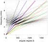 |
Fig. 3 Power spectrum of the vertical velocity at log τ = 0.01 from the quiet Sun simulation. The gray-scale represents the power from low (white) to high (black). The thin dashed lines indicate the position of the eigenfrequencies of the f and p modes in model S. The thick dashed line illustrates the region where the phase speed is equal to the sound speed at the bottom boundary of the model. Regions between lines with the same color correspond to the range in phase speed spanned by phase-speed filters TD2 (orange), TD3 (green), TD4 (red), and TD5 (dark blue). The horizontal dotted lines at constant frequency mark the bandpass regions of the frequency filters. |
Figure 3 illustrates the power spectra of the quiet-Sun simulation, with the model S (Christensen-Dalsgaard et al. 1996) eigenfrequencies of the f mode and p1 to p4 modes overplotted as a reference. The regions in the k − ω domain spanned by the frequency and phase-speed filters are indicated.
3. Travel-time shift measurements
3.1. Maps
The dependence of the travel-time shifts with frequency and phase speed (positive values for low frequencies and low phase speeds and negative values for high frequencies and high phase speeds) is in qualitative agreement with the results obtained from actual observations (Braun & Birch 2008; Braun et al. 2012) and previous numerical simulations (Moradi et al. 2009; Braun et al. 2012; Felipe et al. 2016). Figures 4–6 illustrate the travel-time shift maps of the three simulations with a Wilson depression of 550 km. We do not show the maps for the other sunspot cases, since their qualitative behavior is similar and the quantitative differences are better appreciated in the radial-average plots in the following sections.
3.1.1. TD4 and TD5 phase-speed filters
Negative travel-time shifts are obtained for the phase-speed filters TD4 and TD5 for all frequencies in all of our sunspot models. The magnitude depends on the phase speed and frequency. In the case of the sunspot with Bu = 3500 G(Fig. 6), the maximum travel-time perturbation is found for the phase-speed filter TD4 and frequency of 3.25 mHz. Higher frequencies show a lower magnitude in the travel time perturbation. On the contrary, the sunspot with the lowest magnetic field strength (Fig. 4) shows stronger perturbations for high frequencies. For those filter combinations (high phase speed and high frequency) the travel-time perturbation is reduced in amplitude with increasing magnetic field (considering the same Wilson depression).
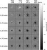 |
Fig. 4 Maps of travel-time shifts obtained for the sunspot model with Bu = 1500 G and zWD = 550 km using phase speed and frequency bandpass filters. Each column corresponds to a different phase-speed filter (the name of the filter and its phase speed in km s-1 are indicated at the top). The rows correspond to frequency filters (increasing from 2.75 mHz in the top row to 5.25 mHz in the bottom row). |
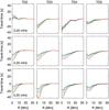 |
Fig. 7 Radial variation of the azimuthally averaged travel-time shifts measured for the simulations with Bu = 1500 G and zWD = 250 km (black), zWD = 350 km (blue), zWD = 450 km (green), or zWD = 550 km (red). The columns correspond to different phase-speed filters, from lower phase speed (left panels) to higher phase speed (right panels). The rows correspond to frequency filters centered at 3.25 mHz (top panels), 4.25 mHz (middle panels), and 5.25 mHz (bottom panels). The errors bars shown represent an assessment of measurement errors of the travel-time shift differences between two models (see text). |
3.1.2. TD2 and TD3 phase-speed filters
The travel-time shifts for low phase-speed filters (TD2 and TD3) changes from positive values (waves apparently slower in the sunspot than in the quiet Sun) to negative values (faster waves in the sunspot) as the frequency increases. The frequency at which this sign reversal is produced is lower for the TD3 filter than for the TD2 filter, but it also depends on the sunspot model. For the sunspot with Bu = 3500 Gand zWD = 550 km(Fig. 6), the travel-time shift measured at 2.75 mHz and TD3 is mainly positive, while a 3.25 mHz frequency shows a mix of positive and negative shifts. In the other two sunspots with lower field strengths (Figs. 4 and 5), this combination of filters produces a negative travel-time shift, which is especially prominent in the case with Bu = 1500 G. For the TD3 case, higher frequencies are clearly negative in the three sunspots shown in Figs. 4–6. With regards to TD2 phase-speed filter, in the sunspot with stronger magnetic field negative travel-time shifts are found for frequencies higher than 4 mHz. For the sunspots with Bu = 1500, 2500 G, the travel-time shift of waves with 3.75 mHz frequency and phase speed given by TD2 filter shows a negative value surrounded by an annular region with positive shift. For higher frequencies the positive ring vanishes, and only the negative signal remains.
3.2. Sensitivity to the Wilson depression
We computed azimuthally averaged travel-time shifts for all of the sunspot models. Figure 7 shows the radial variation of the averaged travel-time shifts for some selected frequencies for all the simulations with Bu = 1500 G. To assess the significance of differences between measurements of the travel-time shifts among the models, we compute errors in the following manner. We first take the difference between the travel-time shift maps for two models with different values of the Wilson depression. Although the same distribution of acoustic sources are used to reduce the realization noise (see Sect. 2), a residual amount of noise remains. The map of the travel-time shift difference is divided into four quadrants centered on the sunspot and the error is estimated as the total spread (maximum minus minimum value) of the four azimuthal averages within each individual quadrant (all of the models considered here are cylindrically symmetric, meaning that any variations between quadrants is due to noise). In order to simplify the figure, only the errors of the difference between the zWD = 350 km and 450 km cases are shown, superimposed on the zWD = 350 km measurements. Errors computed using other pairs of models are similar. As expected, the measured signal increases in amplitude with the Wilson depression. An increase of the Wilson depression produces a shift in the depth of the upper turning point of the waves toward deeper layers. As a result, the path traveled by wave rays hitting the center of the sunspot is shorter than that of waves reaching the photosphere in quiet-Sun regions. This effect leads to shorter travel times in the sunspot, and the magnitude of this reduction is stronger for more depressed sunspot atmospheres.
3.2.1. Frequency dependence
Most of the averaged travel-time shifts illustrated in Fig. 7show a negative travel-time shift. Only the case with TD2 and 3.25 mHz frequency (and lower frequencies with phase speed given by TD2 and TD3, as seen in Fig. 4) produces a positive perturbation in the travel time. It is interesting to note that this positive perturbation increases with the Wilson depression. In this case, the variation of the travel time cannot be understood as the result of the changes in the depth of the upper turning point.
The sensitivity of the travel-time shift to the Wilson depression depends on the combination of filters used for the measurement. The travel-time shift measured for waves with 3.25 mHz frequency at the central part of the umbra shows differences around 7 s at most between the results obtained for the case with zWD = 250 kmand the case with zWD = 550 km. On the contrary, for waves with 5.25 mHz frequency this variation can be larger than 25 s, as found for the phase-speed filter TD3. The top panel of Fig. 1 shows the vertical stratification of the cut-off frequency from the Bu = 1500 Gcases, whose travel-time shifts are plotted in Fig. 7. A wave with 3.25 mHz frequency (bottom horizontal dashed line) propagating upward from the interior will reach the turning point of the zWD = 550 kmmodel (red line) earlier than that of the smaller Wilson depression models. Waves propagating in sunspot models with small Wilson depression will travel a longer path, closer to that traveled in a quiet-Sun region (thick black dashed line). The difference in the depth where the cut-off frequency is 3.25 mHz between the zWD = 250 kmand zWD = 550 kmcases is around 220 km, in the sense that the path of the latter is shorter. For waves with 5.25 mHz, the reduction of the travel path is more than 300 km, producing a larger difference in the travel-time perturbation signal. This effect can qualitatively explain the dependence of the travel-time shift on the frequency for models with the same field strength.
The variation of the travel-time signal with the Wilson depression at constant field strength shows a similar trend for the case with Bu = 3500 G(Fig. 8), although filters TD3 and TD4 show a weaker dependence at high frequencies. The results for the model with Bu = 2500 G(not shown in figures) are somewhat between the other two cases.
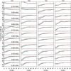 |
Fig. 9 Radial variation of the azimuthally averaged travel-time shifts measured for the simulations with zWD = 450 km and Bu = 1500 G (black), Bu = 2500 G (blue), or Bu = 3500 G (red). The green dashed line corresponds to the results for a sunspot with the thermal structure of the model with Bu = 2500 G and zWD = 450 km but with the magnetic field set to zero (see Felipe et al. 2016). The columns correspond to different phase-speed filters, from lower phase speed (left panels) to higher phase speed (right panels). The rows correspond to frequency filters with increasing frequency from top to bottom. The errors bars shown represent an assessment of measurement errors of the travel-time shift differences between two models (see text). |
3.3. Sensitivity to the magnetic field strength
Figure 9 shows the azimuthally averaged travel-time shift measured for the simulations with a Wilson depression of 450 km, but with different magnetic field strengths. Errors are estimated for differences in measurements using models with different magnetic field strength in a manner similar to that discussed in Sect. 3.2. Shown are errors of the difference between measurements from the Bu = 2500 Gand the Bu = 1500 Gmodels, superimposed on the Bu = 2500 Gmeasurements. Errors computed using other pairs of models are similar. The largest differences between models are found for the TD2 filter and frequencies between 3.25 and 4.00 mHz. In that region the magnetic field causes changes in the travel-time shift of around 30 s, and the perturbations can even show an opposite sign, as seen in Sect. 3.1. For example, TD2 waves with 3.50 mHz frequency show a negative travel-time shift for the sunspot with Bu = 1500 Gbut a positive shift for the other two cases. The dashed green lines illustrate the signal obtained from a background model with the density, pressure, and coefficient of specific heats from the sunspot with Bu = 2500 Gand zWD = 450 kmbut with the magnetic field set to zero. These data correspond to the “thermal sunspot” analyzed in Felipe et al. (2016).
3.3.1. Low frequencies
The travel-time shifts at lower frequencies (2.75 mHz for all the phase-speed filters and also 3.00 mHz for TD2) show a weak dependence on the magnetic field strength. For most phase-speed filters and radial positions it is below the error of the measurement procedure. The change in the travel-time shift between models with Bu = 1500 Gand 3500 G is only measurable for the phase-speed filter TD2 near the center of the sunspots and for TD4. In all the sunspot models, the upper turning point for low frequencies is deeper than the depth where β = 1 (Fig. 1). Upward-propagating waves with low frequencies reach the turning point before the magnetic effects are relevant. They neither reach the mode conversion layer nor propagate at depths where the fast speed is significantly modified by the increase of the Alfvén velocity.
3.3.2. Intermediate frequencies
For frequencies between 3.00 and 3.25 mHz, the negative travel-time perturbations measured with the higher phase-speed filters (TD4 and TD5) increase with the strength of the magnetic field. The case with Bu = 3500 Gshows shifts around –40 s for the TD4 filter at the central part of the umbra. The magnitude of the shift is lower for the Bu = 2500 Gand Bu = 1500 G, but a comparison of the latter with the thermal sunspot reveals a perfect match. Interestingly, although the travel-time perturbations for frequencies between 3.00 mHz and 3.75 mHz are sensitive to the field strength, the thermal sunspot produces signals in quantitative agreement with the sunspot with Bu = 1500 G(except for TD2 filter). That is, the travel times are nearly insensitive to changes in the magnetic field for strengths below 1500 G. As can be seen in Fig. 1, the distance between the turning point and the β = 1 depth decreases with the magnetic field strength. Waves with frequency around 3.00 mHz propagating through the Bu = 2500 Gand Bu = 3500 Gmodels can be affected by the magnetic effects, but in the Bu = 1500 Gmodel they do not reach the region where these effects are significant. The shorter travel times for the strongly magnetized sunspots agree with the faster propagation velocity in those models, since their fast magnetoacoustic speed is higher than for the low-field-strength model. This situation differs from the TD2 and TD3 cases with frequencies between 3.25 mHz and 4.00 mHz, where the models with strong magnetic field show longer travel times. In those cases the interaction with the magnetic field is more complex and must be associated with the larger angle of incidence of those waves, since the lower-phase-speed waves propagate in a shallower cavity.
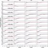 |
Fig. 10 Radial variation of the azimuthally averaged travel-time shifts between models with zWD = 450 km and models with zWD = 250 km. The line color indicates the magnetic field strength of the pair of models: Bu = 1500 G (black), Bu = 2500 G (blue), or Bu = 3500 G (red). Negative (positive) differences correspond to shorter (longer) travel times in the model with zWD = 450 km. |
3.3.3. High frequencies
The travel-time shifts measured with all phase-speed filters show a slight variation with magnetic field for high frequencies (generally around 10 s). In these cases the magnitude of the perturbation decreases with the field strength, opposite to the results found for low frequency and high-phase-speed waves. The differences between the Bu = 1500 Gand Bu = 2500 Gcases are small but higher than the value of the measurement error. The travel time obtained for the stronger magnetic field simulation is clearly distinguishable from the other two cases. However, the “thermal sunspot” shows a quantitative agreement with the sunspot model with Bu = 2500 Gand zWD = 450 km. These two simulations have exactly the same thermal structure; they only differ in the absence of magnetic field in the former. Their comparison implies that a 2500 G field strength change does not produce significant changes in the travel time. Instead, the variations identified between the three models with different field strength must be due to the differences in their thermal structure, even though they have the same Wilson depression. The construction of the MHS models requires the imposition of force balance. The magnetic force is different in the three models and, thus, their thermal structure must necessarily differ. The three models have the same Wilson depression, but show differences in the stratification of pressure, density and coefficient of specific heat which lead to differences in their sound speed, as shown in Fig. 2. The sound speed in the layers between z = − 1.7 Mm and z = − 0.7 Mm decreases with increasing field strength. p-mode waves propagating through the Bu = 1500 Gsunspot will be faster than waves in the other sunspots, leading to the reduced travel time measured for high frequencies in this model.
The frequency above which the travel-time perturbations can be interpreted as a result of the changes in the Wilson depression and sound speed rather than magnetic field depend of the phase-speed filter. For the TD2 case the threshold is at 4.25 mHz, for TD3 at 4.00 mHz, and for TD4 and TD5 filters at 3.75 mHz.
Models with other values for the Wilson depression show a similar dependence on the magnetic field strength. The results of these cases are in qualitative agreement with those illustrated in Fig. 9. Figure 10 shows the travel-time shift between models with zWD = 450 kmand models with zWD = 250 km. That is, it is equivalent to Fig. 9 except that the travel times of the zWD = 250 kmcases were subtracted instead of the travel times obtained from the quiet-Sun simulation. This representation highlights the differences between pairs of sunspot models. A negative travel-time shift indicates that the travel time of the waves in the simulation with zWD = 450 kmis shorter and vice versa. In the cases with small Wilson depression, the dependence of the high frequency travel times on the magnetic field strength is lower, since the difference in the sound speed is smaller than in the zWD = 450 kmcases (shown by comparison of the first and third panels of Fig. 2).
4. Discussion and conclusions
We have performed a parametric study of the sensitivity of the travel-time shifts measured using helioseismic holography to sunspot models with different Wilson depressions and magnetic field strengths. This study is a continuation of the paper Felipe et al. (2016). The results confirm those from the previous work and reveal new findings. Our main conclusions are:
-
The Wilson depression has a strong effect on the measuredtravel-time shifts. The depression of the atmosphere lowers theheight of the upper turning point of the waves, and the path theytravel beneath the sunspot is shorter than that of waves inquiet-Sun regions. This causes a reduction in the travel time. Themagnitude of the reduction increases with the Wilson depression(Figs. 7 and 8). Low frequenciesare less sensitive to this effect, since the change in the depth of theirupper turning point is smaller than for high-frequency waves(Fig. 1).
-
Waves with frequencies below 3.00 mHz show a weak dependence on the magnetic field strength. Their cut-off height is below the region where magnetic field effects are significant. In the case of the TD4 and TD5 phase-speed filters, they show a negative travel-time perturbation, which is in agreement with the deeper turning point of those waves in the sunspot models with respect to the quiet-Sun atmosphere. This is opposite to the positive shifts obtained for the low phase-speed filters (TD2 and TD3). Braun & Birch (2008) and Birch et al. (2009) have argued that this sign change is a property of the chosen data analysis filters.
-
The direct effects of the magnetic field on the travel time are apparent for some combinations of phase speed and frequency filters. For the phase-speed filter TD2, the travel-time perturbation measured for frequencies between 3.25 and 4.00 mHz is clearly modified by the magnetic field strength. For the filter TD3, waves with frequencies between 3.00 and 3.75 mHz are sensitive to the magnetic field, while the filters TD4 and TD5 show variation of the travel-time shift with magnetic field for frequencies between 3.00 and 3.50 mHz. These conclusions are based on the analysis of the sunspots with a Wilson depression of 450 km (Fig. 9), but the results are similar for the other models.
-
For all phase-speed filters analyzed, the travel-time perturbation at high frequencies is likely caused by the changes in the thermal model. The Wilson depression shortens the path of the waves, reducing the travel times. However, the Wilson depression on its own cannot account for the obtained travel-time shifts. The variation of the sound speed (among models with the same Wilson depression) at depths between z = − 1.7 Mm and z = − 0.7 Mm is also measurable, and is responsible for changes of around 10 s in the travel time (see Fig. 9).
-
The travel-time shift is insensitive to the direct effects of photospheric magnetic field strengths below 1500 G. As indicated in the previous bullet point, travel-times at high frequencies are insensitive to the magnetic field. Only low frequencies depend on the field strength, but for those filters the travel-time perturbation measured from the sunspot with Bu = 1500 G shows a perfect match with the “thermal sunspot”, whose magnetic field vanishes (Fig. 9). For small sunspots and pores, the only contribution to the travel time comes from the indirect effect of the magnetic field on the thermal structure, through changes in the sound speed and Wilson depression.
We have used a set of forward calculations to show examples of how travel times depend on the properties of various sunspot models. We emphasize that the model sunspots described in this paper are not intended to represent any particular observed sunspot (for example, by matching the observed sunspot radius or radial profile of magnetic field) and it would therefore be premature to compare the modeled travel times with observed sunspot travel times. It is, however, important to know which of these travel-time variations are detectable above the observational noise levels. Figure 9 from Braun et al. (2012) shows the umbral averages (and errors) of the travel-time shifts measured in the sunspot in AR11092 using 24 h of Helioseismic and Magnetic Imager (HMI; Schou et al. 2012) data. The error they retrieved is below 10 s for all the phase-speed and frequency filters, while for some filter combinations (especially for TD4) the measured error is significantly lower (below 5 s). For photospheric umbral magnetic field around or below 2500 G, the change in the travel-time perturbation produced by 100 km shifts in the Wilson depression could be detected above the noise level in the TD3 and TD4 filters for frequencies around 5 mHz (Fig. 7). Models with Bu = 3500 G do not show such a strong travel time variation with Wilson depression at high frequencies (Fig. 8), and the precision of the Wilson depression estimation would be lower. For other filter combinations the observational noise is comparable or above the travel-time shift associated to changes in the Wilson depression.
The highest sensitivity of the travel-time shift to the Wilson depression is obtained for the phase-speed filter TD3 at 5.25 mHz. This combination of phase-speed and frequency filters encompasses the ridge of the p2 mode (Fig. 3). This is in general agreement with Schunker et al. (2013), who concluded that p2 waves are a good candidate for constraining the depth of the Wilson depression. We also find that the phase-speed filter TD4 at 5.25 mHz (p3 mode) is another good candidate for measuring the Wilson depression. This mode was not considered by Schunker et al. (2013).
The travel-time shifts caused mainly by the changes in the sound speed among models with the same Wilson depression but different field strengths (high frequencies, Fig. 9) are also above the observational noise level when the sound speed perturbation is high enough (sound speed changes between models with Bu = 3500 G and Bu = 1500 G). Schunker et al. (2013) evaluated the sensitivity of the travel time of p1 waves to sound-speed perturbations located at z = − 1.5 Mm (close to the depth of the sound-speed perturbation in our models). They found that the p1 travel-time shift is below the observed noise level, even for cases with a sound speed perturbation much higher than that introduced in our models. Our results are more sensitive to the changes in the sound-speed because they include higher-order p modes (according to the phase-speed and frequency filters used in this work, we have measured up to p4). Interestingly, we found that the lowest frequency for which the travel-time shifts depend on the sound-speed perturbation decreases with increasing phase speed, which agrees with the fact that higher phase-speed filters are sensitive to higher order p modes at lower frequencies (see Fig. 3). The depth sensitivity of p2 to p4 modes provides a better sampling of the region where the sound-speed perturbation is located in our models.
Felipe et al. (2016) suggested a path toward simplified travel-time inversion methods by selecting some combinations of phase-speed and frequency filters that are less sensitive to the magnetic field. The inversion should account for the changes in the Wilson depression and sound speed. This approach would
eliminate the need to compute the sensitivity of wave travel times to the strength and geometry of the magnetic field (e.g., Hanasoge et al. 2012). Our results support this suggestion.
Acknowledgments
We acknowledge the financial support of the Spanish Ministry of Economy and Competitiveness (MINECO) through projects AYA2014-55078-P, AYA2014-60476-P and AYA2014-60833-P. D.C.B. acknowledges support from the NASA Living With a Star Program through grant NNX14AD42G awarded to NWRA. A.C.B. acknowledges the EU FP7 Collaborative Project “Exploitation of Space Data for Innovative Helio- and Asteroseismology” (SPACEINN). This work used the NASA’s Pleiades supercomputer at Ames Research Center, Teide High-Performance Computing facilities at Instituto Tecnológico y de Energías Renovables (ITER, SA), and MareNostrum supercomputer at Barcelona Supercomputing Center.
References
- Birch, A. C., Braun, D. C., Hanasoge, S. M., & Cameron, R. 2009, Sol. Phys., 254, 17 [NASA ADS] [CrossRef] [Google Scholar]
- Braun, D. C., & Birch, A. C. 2006, ApJ, 647, L187 [NASA ADS] [CrossRef] [Google Scholar]
- Braun, D. C., & Birch, A. C. 2008, Sol. Phys., 251, 267 [NASA ADS] [CrossRef] [Google Scholar]
- Braun, D. C., Duvall, Jr., T. L., Labonte, B. J., et al. 1992, ApJ, 391, L113 [NASA ADS] [CrossRef] [Google Scholar]
- Braun, D. C., Birch, A. C., Rempel, M., & Duvall, T. L. 2012, ApJ, 744, 77 [NASA ADS] [CrossRef] [Google Scholar]
- Cally, P. S. 2009, MNRAS, 395, 1309 [NASA ADS] [CrossRef] [Google Scholar]
- Cally, P. S., & Goossens, M. 2008, Sol. Phys., 251, 251 [NASA ADS] [CrossRef] [Google Scholar]
- Cally, P. S., & Hansen, S. C. 2011, ApJ, 738, 119 [NASA ADS] [CrossRef] [Google Scholar]
- Cally, P. S., & Moradi, H. 2013, MNRAS, 435, 2589 [NASA ADS] [CrossRef] [Google Scholar]
- Cameron, R., Gizon, L., & Duvall, Jr., T. L. 2008, Sol. Phys., 251, 291 [NASA ADS] [CrossRef] [Google Scholar]
- Cameron, R. H., Gizon, L., Schunker, H., & Pietarila, A. 2011, Sol. Phys., 268, 293 [NASA ADS] [CrossRef] [Google Scholar]
- Christensen-Dalsgaard, J., Dappen, W., Ajukov, S. V., et al. 1996, Science, 272, 1286 [CrossRef] [Google Scholar]
- Couvidat, S., & Rajaguru, S. P. 2007, ApJ, 661, 558 [NASA ADS] [CrossRef] [Google Scholar]
- Couvidat, S., Birch, A. C., & Kosovichev, A. G. 2006, ApJ, 640, 516 [NASA ADS] [CrossRef] [Google Scholar]
- Duvall, Jr., T. L., Jefferies, S. M., Harvey, J. W., & Pomerantz, M. A. 1993, Nature, 362, 430 [NASA ADS] [CrossRef] [Google Scholar]
- Duvall, Jr., T. L., Kosovichev, A. G., Scherrer, P. H., et al. 1997, Sol. Phys., 170, 63 [NASA ADS] [CrossRef] [Google Scholar]
- Fan, Y., Braun, D. C., & Chou, D.-Y. 1995, ApJ, 451, 877 [NASA ADS] [CrossRef] [Google Scholar]
- Felipe, T. 2012, ApJ, 758, 96 [NASA ADS] [CrossRef] [Google Scholar]
- Felipe, T., Khomenko, E., & Collados, M. 2010, ApJ, 719, 357 [Google Scholar]
- Felipe, T., Braun, D. C., Crouch, A. D., & Birch, A. C. 2016, ApJ, 829, 67 [NASA ADS] [CrossRef] [Google Scholar]
- Hanasoge, S., Birch, A., Gizon, L., & Tromp, J. 2012, Phys. Rev. Lett., 109, 101101 [NASA ADS] [CrossRef] [Google Scholar]
- Hansen, S. C., & Cally, P. S. 2012, ApJ, 751, 31 [NASA ADS] [CrossRef] [Google Scholar]
- Khomenko, E., & Cally, P. S. 2012, ApJ, 746, 68 [NASA ADS] [CrossRef] [Google Scholar]
- Khomenko, E., & Collados, M. 2006, ApJ, 653, 739 [Google Scholar]
- Khomenko, E., & Collados, M. 2008, ApJ, 689, 1379 [NASA ADS] [CrossRef] [Google Scholar]
- Kosovichev, A. G. 1996, ApJ, 461, L55 [NASA ADS] [CrossRef] [Google Scholar]
- Kosovichev, A. G., Duvall, Jr., T. L., & Scherrer, P. H. 2000, Sol. Phys., 192, 159 [NASA ADS] [CrossRef] [Google Scholar]
- Lindsey, C., & Braun, D. C. 2005, ApJ, 620, 1107 [NASA ADS] [CrossRef] [Google Scholar]
- Low, B. C. 1980, Sol. Phys., 67, 57 [NASA ADS] [CrossRef] [Google Scholar]
- Moradi, H., Hanasoge, S. M., & Cally, P. S. 2009, ApJ, 690, L72 [NASA ADS] [CrossRef] [Google Scholar]
- Moradi, H., Cally, P. S., Przybylski, D., & Shelyag, S. 2015, MNRAS, 449, 3074 [NASA ADS] [CrossRef] [Google Scholar]
- Pizzo, V. J. 1986, ApJ, 302, 785 [NASA ADS] [CrossRef] [Google Scholar]
- Rempel, M., Schüssler, M., & Knölker, M. 2009, ApJ, 691, 640 [NASA ADS] [CrossRef] [Google Scholar]
- Rosenthal, C. S., Bogdan, T. J., Carlsson, M., et al. 2002, ApJ, 564, 508 [NASA ADS] [CrossRef] [Google Scholar]
- Schou, J., Scherrer, P. H., Bush, R. I., et al. 2012, Sol. Phys., 275, 229 [Google Scholar]
- Schunker, H., & Cally, P. S. 2006, MNRAS, 372, 551 [NASA ADS] [CrossRef] [Google Scholar]
- Schunker, H., Braun, D. C., Cally, P. S., & Lindsey, C. 2005, ApJ, 621, L149 [NASA ADS] [CrossRef] [Google Scholar]
- Schunker, H., Gizon, L., Cameron, R. H., & Birch, A. C. 2013, A&A, 558, A130 [NASA ADS] [CrossRef] [EDP Sciences] [Google Scholar]
- Werne, J., Birch, A., & Julien, K. 2004, in SOHO 14 Helio- and Asteroseismology: Towards a Golden Future, ed. D. Danesy, ESA SP, 559, 172 [NASA ADS] [Google Scholar]
- Zhao, J., Kosovichev, A. G., & Duvall, Jr., T. L. 2001, ApJ, 557, 384 [NASA ADS] [CrossRef] [Google Scholar]
All Figures
|
Fig. 1 Vertical stratification of the isothermal cut-off frequency at the axis of the sunspot models with Bu = 1500 G (top panel), Bu = 2500 G (middle panel), and Bu = 3500 G (bottom panel), where z is height and z = 0 is defined at the quiet-Sun photosphere. The colored lines correspond to the Wilson depression of the model: zWD = 250 km (black), zWD = 350 km (blue), zWD = 450 km (green), and zWD = 550 km (red). The vertical dotted lines illustrate the height where β = 1 for the model with the Wilson depression associated to the corresponding color. The horizontal thin dashed lines mark some selected frequencies (3.25, 4.25, 5.25 mHz). The thick black dashed line illustrates the cut-off frequency at the quiet-Sun. |
| In the text | |
|
Fig. 2 Vertical stratification of the sound speed at the axis of the sunspot models with zWD = 250 km (top panel), zWD = 350 km (second panel), zWD = 450 km (third panel), and zWD = 550 km (bottom panel), where z is height and z = 0 is defined at the quiet-Sun photosphere. The color of the lines indicates the photospheric umbral magnetic field strength of the model: Bu = 1500 G km (black), Bu = 2500 G (blue), and Bu = 3500 G km (red). The vertical dotted lines illustrate the height where β = 1 for the model with the magnetic field associated to the corresponding color. The thick black dashed line illustrates the sound speed in the quiet Sun. |
| In the text | |
|
Fig. 3 Power spectrum of the vertical velocity at log τ = 0.01 from the quiet Sun simulation. The gray-scale represents the power from low (white) to high (black). The thin dashed lines indicate the position of the eigenfrequencies of the f and p modes in model S. The thick dashed line illustrates the region where the phase speed is equal to the sound speed at the bottom boundary of the model. Regions between lines with the same color correspond to the range in phase speed spanned by phase-speed filters TD2 (orange), TD3 (green), TD4 (red), and TD5 (dark blue). The horizontal dotted lines at constant frequency mark the bandpass regions of the frequency filters. |
| In the text | |
|
Fig. 4 Maps of travel-time shifts obtained for the sunspot model with Bu = 1500 G and zWD = 550 km using phase speed and frequency bandpass filters. Each column corresponds to a different phase-speed filter (the name of the filter and its phase speed in km s-1 are indicated at the top). The rows correspond to frequency filters (increasing from 2.75 mHz in the top row to 5.25 mHz in the bottom row). |
| In the text | |
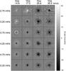 |
Fig. 5 Same as Fig. 4 but for the sunspot with Bu = 2500 G and zWD = 550 km. |
| In the text | |
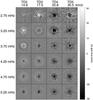 |
Fig. 6 Same as Fig. 4 but for the sunspot with Bu = 3500 G and zWD = 550 km. |
| In the text | |
|
Fig. 7 Radial variation of the azimuthally averaged travel-time shifts measured for the simulations with Bu = 1500 G and zWD = 250 km (black), zWD = 350 km (blue), zWD = 450 km (green), or zWD = 550 km (red). The columns correspond to different phase-speed filters, from lower phase speed (left panels) to higher phase speed (right panels). The rows correspond to frequency filters centered at 3.25 mHz (top panels), 4.25 mHz (middle panels), and 5.25 mHz (bottom panels). The errors bars shown represent an assessment of measurement errors of the travel-time shift differences between two models (see text). |
| In the text | |
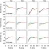 |
Fig. 8 Same as Fig. 7 but for sunspot models with Bu = 3500 G. |
| In the text | |
|
Fig. 9 Radial variation of the azimuthally averaged travel-time shifts measured for the simulations with zWD = 450 km and Bu = 1500 G (black), Bu = 2500 G (blue), or Bu = 3500 G (red). The green dashed line corresponds to the results for a sunspot with the thermal structure of the model with Bu = 2500 G and zWD = 450 km but with the magnetic field set to zero (see Felipe et al. 2016). The columns correspond to different phase-speed filters, from lower phase speed (left panels) to higher phase speed (right panels). The rows correspond to frequency filters with increasing frequency from top to bottom. The errors bars shown represent an assessment of measurement errors of the travel-time shift differences between two models (see text). |
| In the text | |
|
Fig. 10 Radial variation of the azimuthally averaged travel-time shifts between models with zWD = 450 km and models with zWD = 250 km. The line color indicates the magnetic field strength of the pair of models: Bu = 1500 G (black), Bu = 2500 G (blue), or Bu = 3500 G (red). Negative (positive) differences correspond to shorter (longer) travel times in the model with zWD = 450 km. |
| In the text | |
Current usage metrics show cumulative count of Article Views (full-text article views including HTML views, PDF and ePub downloads, according to the available data) and Abstracts Views on Vision4Press platform.
Data correspond to usage on the plateform after 2015. The current usage metrics is available 48-96 hours after online publication and is updated daily on week days.
Initial download of the metrics may take a while.