| Issue |
A&A
Volume 604, August 2017
|
|
|---|---|---|
| Article Number | A134 | |
| Number of page(s) | 26 | |
| Section | Catalogs and data | |
| DOI | https://doi.org/10.1051/0004-6361/201730747 | |
| Published online | 28 August 2017 | |
The third data release of the Kilo-Degree Survey and associated data products
1 Leiden Observatory, Leiden University, PO Box 9513, 2300 RA Leiden, The Netherlands
e-mail: This email address is being protected from spambots. You need JavaScript enabled to view it.
2 Kapteyn Astronomical Institute, University of Groningen, PO Box 800, 9700 AV Groningen, The Netherlands
3 Argelander-Institut für Astronomie, Auf dem Hügel 71, 53121 Bonn, Germany
4 INAF – Osservatorio Astronomico di Capodimonte, via Moiariello 16, 80131 Napoli, Italy
5 National Centre for Nuclear Research, Astrophysics Division, PO Box 447, 90-950 Łódź, Poland
6 Department of Physics “E. Pancini”, University Federico II, via Cinthia 6, 80126 Napoli, Italy
7 INAF – Osservatorio Astronomico di Padova, via dell’Osservatorio 5, 35122 Padova, Italy
8 Scottish Universities Physics Alliance, Institute for Astronomy, University of Edinburgh, Royal Observatory, Blackford Hill, Edinburgh, EH9 3HJ, UK
9 Centre for Astrophysics & Supercomputing, Swinburne University of Technology, PO Box 218, Hawthorn, VIC 3122, Australia
10 Center for Cosmology and AstroParticle Physics, The Ohio State University, 191 West Woodruff Avenue, Columbus, OH 43210, USA
11 Institute of Space Sciences and Astronomy (ISSA), University of Malta, Msida, MSD 2080, Malta
12 Department of Physics, University of Malta, Msida, MSD 2080, Malta
13 Canadian Astronomy Data Centre, Herzberg Astronomy and Astrophysics, 5071 West Saanich Road, Victoria, BC, V9E 2E7, Canada
14 Department of Physics, University of Oxford, Keble Road, Oxford OX1 3RH, UK
Received: 8 March 2017
Accepted: 12 May 2017
Abstract
Context. The Kilo-Degree Survey (KiDS) is an ongoing optical wide-field imaging survey with the OmegaCAM camera at the VLT Survey Telescope. It aims to image 1500 square degrees in four filters (ugri). The core science driver is mapping the large-scale matter distribution in the Universe, using weak lensing shear and photometric redshift measurements. Further science cases include galaxy evolution, Milky Way structure, detection of high-redshift clusters, and finding rare sources such as strong lenses and quasars.
Aims. Here we present the third public data release and several associated data products, adding further area, homogenized photometric calibration, photometric redshifts and weak lensing shear measurements to the first two releases.
Methods. A dedicated pipeline embedded in the Astro-WISE information system is used for the production of the main release. Modifications with respect to earlier releases are described in detail. Photometric redshifts have been derived using both Bayesian template fitting, and machine-learning techniques. For the weak lensing measurements, optimized procedures based on the THELI data reduction and lensfit shear measurement packages are used.
Results. In this third data release an additional 292 new survey tiles (≈300 deg2) stacked ugri images are made available, accompanied by weight maps, masks, and source lists. The multi-band catalogue, including homogenized photometry and photometric redshifts, covers the combined DR1, DR2 and DR3 footprint of 440 survey tiles (44 deg2). Limiting magnitudes are typically 24.3, 25.1, 24.9, 23.8 (5σ in a 2′′ aperture) in ugri, respectively, and the typical r-band PSF size is less than 0.7′′. The photometric homogenization scheme ensures accurate colours and an absolute calibration stable to ≈2% for gri and ≈3% in u. Separately released for the combined area of all KiDS releases to date are a weak lensing shear catalogue and photometric redshifts based on two different machine-learning techniques.
Key words: surveys / catalogs / techniques: photometric / techniques: image processing
© ESO, 2017
1. The Kilo-Degree Survey
With the advent of specialized wide-field telescopes and cameras, large multi-wavelength astronomical imaging surveys have become important tools for astrophysics. In addition to the specific scientific goals that they are designed and built for, their data have huge legacy value and facilitate a large variety of scientific analyses. For these reasons, since their commissioning in 2011 the VLT Survey Telescope (VST, Capaccioli et al. 2012) and its sole instrument, the 268 Megapixel OmegaCAM camera (Kuijken 2011) have been mostly dedicated to three large public surveys1, of which the Kilo-Degree Survey (KiDS, de Jong et al. 2013) is the largest in terms of observing time. It aims to observe 1500 deg2 of extragalactic sky, spread over two survey fields, in four broad-band filters (ugri) (see Fig. 1 and Table 2). Together with its sister survey, the VISTA Kilo-Degree Infrared Galaxy Survey (VIKING, Edge et al. 2013), this will result in a 9-band optical-infrared data set with excellent depth and image quality.
KiDS observing strategy: observing condition constraints and exposure times.
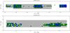 |
Fig. 1 Sky distribution of survey tiles released in KiDS-ESO-DR3 (green) and in the previous releases KiDS-ESO-DR1 and -DR2 (blue). The multi-band source catalogue covers the combined area (blue + green) and the full KiDS area is shown in grey. Top: KiDS-North. Bottom: KiDS-South. Black dashed lines delineate the locations of the GAMA fields; the single pointing at RA = 150°is centred at the COSMOS/CFHTLS D2 field. |
KiDS was designed primarily to serve as a weak gravitational lensing tomography survey, mapping the large-scale matter distribution in the Universe. Key requirements for this application are unbiased and accurate weak lensing shear measurements and photometric redshifts, which put high demands on both image quality and depth, as well as the calibration. The VST-OmegaCAM system is ideal for such a survey, as it was specifically designed to provide superb and uniform image quality over a large, 1° × 1°, field of view (FOV). Combining a science array of 32 thinned, low-noise 2k × 4k E2V devices, a constant pixel scale of 0.21′′, and real-time wave-front sensing and active optics, the system provides a PSF equal to the atmospheric seeing over the full FOV down to 0.6′′. To achieve optimal shear measurements, the survey makes use of the flexibility of service mode scheduling. Observations in the r band are taken under the best dark-time conditions, with g and u in increasingly worse seeing. The i band is the only filter observed in bright time. The observing condition constraints for execution of KiDS OBs are listed in Table 1. Apart from the primary science goal, the KiDS data are exploited for a large range of secondary science cases, including quasar, strong gravitational lens and galaxy cluster searches, galaxy evolution, studying the matter distribution in galaxies, groups and clusters, and even Milky Way structure (e.g. de Jong et al. 2013).
The first two data releases from KiDS (de Jong et al. 2015) became public in 2013 and 2015, containing reduced image data, source lists and a multi-band catalogue for a total of 148 survey tiles (≃160 deg2). Based on this data set, the first scientific results focused on weak lensing studies of galaxies and galaxy groups in the Galaxy And Mass Assembly (GAMA, Driver et al. 2011) fields (Kuijken et al. 2015; Sifón et al. 2015; Viola et al. 2015; Brouwer et al. 2016; van Uitert et al. 2016). Furthermore, these data releases were the basis for the first results from a z ~ 6 quasar search (Venemans et al. 2015), a catalogue of photometric redshifts from machine-learning (Cavuoti et al. 2015, 2017), preliminary results on super-compact massive galaxies (Tortora et al. 2016), and a catalogue of galaxy clusters (Radovich et al. 2017).
In this publication we present the third KiDS data release (KiDS-ESO-DR3). Extending the total released data set to 440 survey tiles (approximately 450 deg2), this release also includes photometric redshifts and a global photometric calibration. In addition to the core ESO release, several associated data products are described that have been released. These include photo-z probability distribution functions, machine-learning photo-z’s, weak lensing shear catalogues and lensing-optimized image data. The first applications of this new data set have appeared already and include the first cosmological results from KiDS (Joudaki et al. 2017; Brouwer et al. 2017; Hildebrandt et al. 2017).
The outline of this paper is as follows. Section 2 is a discussion of the contents of KiDS-ESO-DR3 and the differences in terms of processing and data products with respect to earlier releases. Section 3 presents the weak lensing data products and Sect. 4 reviews the different sets of photometric redshifts that are made available. Data access routes are summarized in Sect. 5 and a summary and outlook towards future data releases is provided in Sect. 6.
2. The third data release
2.1. Content and data quality
KiDS-ESO-DR3 (DR3) constitutes the third data release of KiDS and can be considered an incremental release that adds area, an improved photometric calibration, and photometric redshifts to the two previous public data releases.
In its approximately yearly data releases, KiDS provides data products for survey tiles that have been successfully observed in all four filters (u, g, r, i). Adding 292 new survey tiles to the 50 (DR1) and 98 (DR2) already released tiles, DR3 brings the total released area to 440 tiles. DR3 includes complete coverage of the Northern GAMA fields, which were targeted first, in order to maximize synergy with this spectroscopic survey early on. The distribution of released tiles on the sky is shown in Fig. 1 and a complete list, including data quality information, can be found on the KiDS DR3 website2. For these 292 tiles the following data products are provided for each filter (as they were for DR1 and DR2):
-
astrometrically and photometrically calibrated, stacked images(“coadds”);
-
weight maps;
-
flag maps (“masks”), that flag saturated pixels, reflection halos, read-out spikes, etc.;
-
single-band source lists.
Slight gain variations exist across the FOV, but an average effective gain for each coadd is provided in the tile table on the KiDS DR3 website. The final calibrated, coadded images have a uniform pixel scale of 0.2′′, and the pixel values are in units of flux relative to the flux corresponding to magnitude =0. The magnitude m corresponding to a pixel value f is therefore given by:  (1)The single-band source lists are identical in format and content to those released in DR2 and contain an extensive set of SExtactor (Bertin & Arnouts 1996) based magnitude and geometric measurements, to increase their versatility for the end user. For example, the large number (27) of aperture magnitudes allows users to use interpolation methods (e.g. “curve of growth”) to derive their own aperture corrections or total magnitudes. Also provided are a star-galaxy separation parameter and information on the mask regions that might affect individual source measurements. Table A.1 lists the columns that are present in the single-band source lists provided in KiDS-ESO-DR3.
An aperture-matched multi-band catalogue is also part of DR3. This catalogue covers not only the 292 newly released tiles, but also the 148 tiles released in DR1 and DR2, for a total of 48 736 591 sources in 440 tiles and an area of approximately 447 square degrees. Source detection, positions and shape parameters are all based on the r-band images, since these typically have the best image quality, thus providing the most reliable measurements. The star-galaxy separation provided is the same as that in the r-band single-band source list, and is based on separating point-like from extended sources, which in some tiles yields sub-optimal results due to PSF variations. In future releases we plan to include more information, for example from colours or PSF models, to improve this classification. Magnitudes are measured in all filters using forced photometry. Seeing differences are mitigated in two ways: 1) via aperture-corrected magnitudes, and 2) via Gaussian Aperture and PSF (GAaP) photometry. The latter is new in DR3 and described in more detail in Sect. 2.4. In this release we also introduce a new photometric calibration scheme, based on the GAaP measurements, that homogenizes the photometry in the catalogue over the survey area, using a combination of stellar locus information and overlaps between tiles. The procedures used and the quality of the results are reviewed in Sect. 2.5. Also new in the multi-band catalogue with respect to DR2 are photometric redshifts, see Sect. 4.1. All columns available in this catalogue are listed in Table A.2.
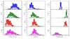 |
Fig. 2 Data quality for KiDS-ESO-DR1 -DR2 and -DR3. Left: average PSF size (FWHM) distributions; centre: average PSF ellipticity distributions; right: limiting magnitude distributions (5σ AB in 2′′ aperture). The distributions are per filter: from top to bottom u, g, r, and i, respectively. The full histograms correspond to the 440 tiles included in the DR3 multi-band catalogue, while the lighter portions of the histograms correspond to fraction (148 tiles) previously released in KiDS-ESO-DR1 and -DR2. |
Data quality of all released tiles.
The intrinsic data quality of the KiDS data is illustrated in Fig. 2 and summarized in Table 3. Average image quality, quantified by the size (FWHM in arcsec) of the point-spread-function (PSF), is driven by the observing constraints supplied to the scheduling system (Table 1). The aim here is to use the best dark conditions for r-band, which is used for the weak lensing shear measurements, with increasingly worse seeing during dark-time allocated to g and u, respectively. The only filter observed in grey and bright time, i-band makes use of a large range of seeing conditions. To improve (relative) data rates in the dark-time filters, the seeing constraints have been relaxed slightly. So far this has not resulted in a significant detrimental effect on the overall image quality of the new DR3 data, when compared to the DR1 and DR2 data. Average ellipticities of stars over the FOV (middle column of Fig. 2), here defined as 1 − b/a and measured by SExtractor (Bertin & Arnouts 1996), are always significantly smaller than 0.1. The depth of the survey is quantified by a signal-to-noise (S/N) of 5σ for point sources in 2′′ apertures. Despite slightly poorer average seeing the g-band data are marginally deeper than the r-band data. The large range of limiting magnitudes in i-band reflects the variety in both seeing and sky illumination conditions. The overall data quality of the DR3 release is very similar to the data quality of DR1 and DR2, as described in de Jong et al. (2015) and Kuijken et al. (2015).
VST baffle configurations.
The most striking and serious issues with the KiDS data are caused by stray light that scatters into the light path and onto the focal plane (see de Jong et al. 2015, for some examples). Over the course of 2014 and 2015, the VST baffles were significantly redesigned and improved (see Table 4). As a result, many of the stray light issues that affect the VST data are now much reduced or eliminated. Although a fraction of the DR3 observations were obtained with improved telescope baffles, the majority of the i-band data, which is most commonly affected, was obtained with the original configuration. Severely affected images are flagged in the tile and catalogue tables on the KiDS DR3 website, and sources in affected tiles are flagged in the multi-band catalogue included in the ESO release.
2.2. Differences with DR1 and DR2
Data processing for KiDS-ESO-DR3 is based on a KiDS-optimized version of the Astro-WISE optical pipeline described in McFarland et al. (2013), combined with dedicated masking and source extraction procedures. The pipeline and procedures used are largely identical to those used for DR2, and for a detailed discussion we refer to de Jong et al. (2015). In the following sections only the differences and additional procedures are described in detail.
2.2.1. Pixel processing
Cross-talk correction. Data processed for DR3 were observed between the 9th of August 2011 and the 4th of October 2015. Since the electronic cross-talk between CCDs #95 and #96 is stable for certain periods, these stable intervals had to be determined for the period following the last observations processed for the earlier releases. The complete set of stable periods and the corrections applied are listed in Table 5.
Applied cross-talk coefficients.
Flatfields and illumination correction. The stray light issues in VST that were addressed with changes to the telescope baffles in 2014 and 2015 do not only affect the science data, but also flatfields. Such additional light present in the flat field results in non-uniform illumination and must be corrected by an “illumination correction” step. Because the illumination of the focal plane changed for each baffle configuration (Table 4), new flat fields and associated illumination corrections are required for each configuration. Thus, whereas for DR1 and DR2 a single set of masterflats was used for each filter, new masterflats were created for each of the baffle configurations. The stability of the intrinsic pixel sensitivities3 still allows a single set to be used for each configuration. Our method to derive the illumination correction makes use of specific calibration observations where the same standard stars are observed with all 32 CCDs (see Verdoes Kleijn et al. 2013). Because such data are not available for all configurations, the differences between the original flatfields and those for each baffle configuration were used to derive new illumination corrections from the original correction.
2.2.2. Masking
Bright stars and related features, such as read-out spikes, diffraction spikes and reflection halos, are masked in the newly released tiles by the Pulecenella software (see de Jong et al. 2015). In prior releases these automated masks were complemented with manual masks that covered a range of other features, including stray light, remaining satellite tracks and reflections/shadows of the covers over the detector heads. Because this way of masking is inherently subjective and not reproducible, and given the considerable effort required, for DR3 we do not provide manual masks. The fraction of masked area in the 292 new tiles is 1.5%, 5.8%, 14.6% and 10.1% in u, g, r and i, respectively. In the 148 tiles released earlier the fraction of automatically masked area was very similar, but the manual masks added a further 2%, 7%, 10% and 14% to this, effectively doubling the total masked area. Using the mask flag values the manual masks in the DR1 and DR2 tiles can be ignored in order to obtain consistent results over the full survey area.
To replace the manually created masks, an automated procedure is under development that aims to identify the same types of areas. This procedure, dubbed MASCS+, will be described in, and the resulting masks released jointly with, a forthcoming paper (Napolitano et al., in prep.).
2.2.3. Photometry and redshifts
The main enhancements of KiDS-ESO-DR3 over DR1 and DR2 are the improved photometric calibration and the inclusion of GAaP (see Kuijken et al. 2015) measurements and photometric redshifts. Where in the earlier releases the released tiles formed a very patchy on-sky distribution, the combined set of 440 survey tiles now available mostly comprises a small number of large contiguous areas, allowing a refinement of the photometric calibration that exploits both the overlap between observations within a filter as well as the stellar colours across filters. This photometric homogenization scheme is the subject of Sect. 2.5.
GAaP is a two-step procedure that homogenizes the PSF over the full FOV of a survey tile, and measures a seeing-independent magnitude in a Gaussian-weighted aperture. This type of measurement yields accurate galaxy colours and approaches PSF-fitting photometry for point sources. See Sect. 2.4 for more details. The colours are used as input for the photometric redshifts included in the DR3 catalogue (Sect. 4), as well as for the machine-learning based photometric redshifts discussed in Sect. 4.
2.3. Additional catalogue columns
Compared to the multi-band catalogue released with KiDS-ESO-DR2, the current multi-band catalogue contains a number of additional columns:
Extinction. For every source the foreground extinction is provided. The colour excess E(B − V) at the source position is transformed to the absorption A in each filter, based on the maps and coefficients by Schlegel et al. (1998). These extinctions can be directly applied to the magnitudes in the catalogue, which are not corrected for extinction.
Tile quality flag. In the absence of manual masking of severe image defects, sources in survey tiles with one or more poor quality coadded images (defined as such during visual inspection of all images) are flagged4. The bitmap value indicates which filter is affected: 1 for u, 2 for g, 4 for r, and 8 for i.
GAaP magnitudes and colours. For each filter the GAaP magnitude for each source is provided, together with the error estimate. The aperture is defined from the r-band image (see Sect. 2.4). Also included are six colours, based on the GAaP magnitudes.
Photometric homogenization. The photometric homogenization procedure (Sect. 2.5) results in zeropoint offsets for each filter in each survey tile. These offsets are included in separate columns and can be applied to the magnitude columns, which are not homogenized. Since the homogenization is based on the GAaP magnitudes, care should be taken when applying these offsets to other magnitude measurements (see Sect. 2.5).
Photometric redshifts. Results from the application of BPZ (Benítez 2000) to the homogenized and extinction-corrected GAaP magnitudes are provided in three columns: i) the best-fitting photometric redshift, ii) the ODDS (Bayesian odds) and iii) the best-fitting spectral template (see Sect. 4 for details).
Astro-WISE identifiers. To enable straightforward cross-matching, and tracing of data lineage with Astro-WISE, the identifiers of the SourceCollections, SourceLists and individual sources therein are propagated.
2.4. Gaussian Aperture and PSF photometry
For some applications, in particular photometric redshifts, reliable colours of each source are needed. For this purpose we provide “Gaussian Aperture and PSF” photometry. These fluxes are defined as the Gaussian-aperture weighted flux of the intrinsic (i.e. not convolved with the seeing PSF) source f(x,y), with the aperture defined by its major and minor axis lengths A and B, and its orientation θ: ![Mathematical equation: \begin{equation} F_{\rm GAaP}=\int\!\!\int {\rm d}x\,{\rm d}y\, f(x,y) {\rm e}^{-[(x'/A)^2+(y'/B)^2]/2} \end{equation}](/articles/aa/full_html/2017/08/aa30747-17/aa30747-17-eq44.png) (3)where x′ and y′ are coordinates rotated by an angle θ with respect to the x and y axes.
(3)where x′ and y′ are coordinates rotated by an angle θ with respect to the x and y axes.
When the PSF is Gaussian, with rms radius p, FGAaP can be related directly to the Gaussian-aperture flux with axis lengths  and
and  , measured on the seeing-convolved image. It thus provides a straightforward way to compensate for seeing differences between different images, and obtain aperture fluxes in different bands that are directly comparable (in the sense that each part of the source gets the same weight in the different bands).
Achieving a Gaussian PSF is done via construction of a convolution kernel that varies across the image, modelled in terms of shapelets (Refregier 2003). The size of the Gaussian PSF is set so as to preserve the seeing as much as possible without deconvolving (which would amplify the noise). The resulting correlation of the pixel noise is propagated into the error estimate on FGAaP. Full details of this procedure are provided in Kuijken et al. (2015, Appendix A).
It is important to note that the GAaP fluxes are primarily intended for colour measurements: because the Gaussian aperture function tapers off they are not total fluxes (except for point sources). As a rule of thumb, for optimal S/N it is best to choose a GAaP aperture that is aligned with the source, and with major and minor axis length somewhat larger than  and
and  . In the KiDS-ESO-DR3 catalogues we set A and B by adding 0.7 arcsec in quadrature to the measured r-band rms major and minor axis radii, with a maximum of 2 arcsec.
2.5. Photometric homogenization
KiDS-ESO-DR3 contains zeropoint corrections for all 440 tiles (1760 coadds) to correct for photometric offsets, for instance due to changes in atmospheric transparency, non-availability of standard star observations during the night (in which case a default is used) or other deviations. The corrections are based on a combination of two methods. The first method is based on the overlaps of adjacent coadds for a particular passband, which we refer to as Overlap Photometry (OP). Out of the 440 tiles, 421 are part of a connected group of 10 or more survey tiles. The second method is a form of stellar locus regression (SLR) and is based on the u,g,r,i colour information of each tile.
The best OP results, determined from comparisons to SDSS DR9 (Ahn et al. 2012) stellar photometry, are obtained for the r-band. SLR works well for g, r and i, but delivers poor results in u-band. Also, SLR provides colour calibration, but no absolute calibration. For these reasons a combination of OP and SLR is used for the overall photometric homogenization. OP is used for a homogeneous, absolute r-band calibration, to which g- and i-band are tied using SLR. For the u-band we solely use an independent OP solution.
2.5.1. Overlap photometry
This method involves homogenizing the calibration within a single passband using overlapping regions of adjacent coadds. Neighbouring coadds have an overlap of 5% in RA and 10% in Dec. The OP calculations used in this release are based on the GAaP photometry (see Sect. 2.4) of point-like objects5. OP can only be used if a tile has sufficient overlap with at least one other tile. This is the case for 431 out of the 440 tiles, leaving 9 isolated tiles (singletons). These 431 tiles are divided over 10 connected groups, which contain 2, 3, 5,10, 20, 50, 65, 89, 92 and 95 members, respectively.
Photometric anchors, observations with reliable photometric calibration, are defined and all other tiles are tied to these. The anchors are selected based on a set of four criteria, that were established based on a comparison of KiDS GAaP magnitudes with SDSS DR9 psfMag measurements. This comparison is limited to the KiDS-North field, since KiDS-South does not overlap with the SDSS footprint. The following four criteria, that depend only on the KiDS data, were found to minimize the magnitude offsets between KiDS and SDSS:
-
1.
initial calibration based on nightly standard star observations;
-
2.
<0.2′′ difference in PSF FWHM with the nightly standard star observation;
-
3.
observed after April 2012 (following the replacement of a faulty video board6);
-
4.
<0.02 mag atmospheric extinction difference between the exposures.
Based on these criteria, in the r-band 45% of all tiles are anchors and in the u-band 18% are. A fitting algorithm is applied to each group and filter independently to minimize the zeropoint differences in the overlaps, with the constraint that the anchor zeropoints should not be changed. Tiles that are singletons receive no absolute calibration correction in either u- or r-band.
2.5.2. Stellar locus regression
The majority of stars form a tight sequence in colour-colour space, the so-called “stellar locus”. Inaccuracies in the photometric calibration of different passbands will shift the location of this stellar locus. Changing the photometric zeropoints such that the stellar locus moves to its intrinsic location should correct these calibration issues. Of course, this procedure only corrects the zeropoints relative to each other, thus providing colour calibration but no absolute calibration. In KiDS-ESO-DR3 SLR is used to calibrate the g − r, and r − i colours which, together with the absolute calibration of the r-band using OP, yields the calibration for g and i.
The intrinsic location of the stellar locus is defined by the “principal colours” derived by Ivezić et al. (2004). In these principal colours, linear combinations of u, g, r and i, straight segments of the stellar locus are centred at 0. Bright, unmasked stars (r< 1) are selected and their GAaP magnitudes corrected for Galactic extinction based on the Schlegel et al. (1998) maps and a standard RV = 3.1 extinction curve7. Per tile the offsets of the straight sections of the stellar locus from 0 in each principal colour are minimized, and the zeropoint offsets converted to three colour offsets: d(u − r), d(g − r) and d(r − i).
Comparing the colours of stars with SDSS measurements provides a straightforward method to assess the improvement in the calibration. In the following, the average colour offsets found between tiles in KiDS-North and SDSS DR9 are used. In g − r the mean per-tile difference between KiDS and SDSS is 6 mmag before SLR and 9 mmag after, but the scatter (standard deviation) decreases from 38 mmag to 12 mmag. Similarly, in r − i the mean offset and scatter change from 16 and 56 mmag to 6 and 11 mmag. Thus, while the absolute colour difference with SDSS remains comparable or improves slightly, the SLR is very successful in homogenizing the colour calibration. For u − r, however, this is not the case, because both the mean colour difference and the scatter are significantly degraded, from 4 and 42 mmag to 80 and 64 mmag. For this reason the results for u − r were not used to calibrate the u-band zeropoints in the DR3 multi-band catalogue, where the u-band thus purely relies on OP. On the other hand, in the KiDS-450 weak lensing shear catalogue (Sect. 3.2) the SLR results were applied in u-band, since no absolute calibration via OP was used in that case. More details of the SLR procedure can be found in Hildebrandt et al. (2017, Appendix B.
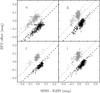 |
Fig. 3 Photometric homogenization zeropoint offsets vs. offsets to SDSS. The offsets calculated by the photometric homogenization procedure are plotted as function of the per-tile offsets of stellar photometry between tiles in KiDS-North and SDSS DR9. Black and grey symbols show the SDSS offsets using GAaP and 10′′ aperture-corrected photometry, respectively, with the dashed lines indicating equality. The GAaP and aperture-corrected data are shifted down and up by 0.05 mag, respectively, to improve the clarity of the figure. Each subpanel corresponds to a different passband, denoted by the labels. |
2.5.3. Accuracy and stability
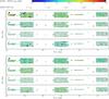 |
Fig. 4 Comparison of KiDS GAaP photometry before and after homogenization to SDSS DR13 for all tiles in KiDS-North as function of right ascension and declination. Top: the magnitude offsets with respect to SDSS before applying photometric homogenization are indicated by the colour scaling. The size of the circles represent the average PSF size in each coadded image. From top to bottom the panels correspond to the u, g, r, and i filters. Bottom: same as top panel, but after applying photometric homogenization. |
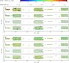 |
Fig. 5 Comparison of KiDS 10′′ aperture-corrected photometry before and after homogenization to SDSS DR13 for all tiles in KiDS-North as function of right ascension and declination. Top: the magnitude offsets with respect to SDSS before applying photometric homogenization are indicated by the colour scaling. The size of the circles represent the average PSF size in each coadded image. From top to bottom the panels correspond to the u, g, r, and i filters. Bottom: same as top panel, but after applying photometric homogenization. |
Comparison of KiDS-North and SDSS DR13 stellar photometry.
The quality of the final photometric homogenization, based on the combination OP for the u- and r-band zeropoint corrections and SLR for the g- and i-band corrections, can be quantified by a direct photometric comparison of KiDS-North to measurements from SDSS. For the comparison presented in this section we use SDSS DR13 (SDSS Collaboration et al. 2016), which includes a new photometric calibration (Finkbeiner et al. 2016) derived from PanSTARRS DR1 (Chambers et al. 2016), the most stable SDSS calibration to date. For this purpose we use stars that are brighter than r = 20, not flagged or masked in KiDS, and that have photometric uncertainties smaller than 0.02 mag in SDSS and the KiDS aperture magnitude in g,r,i and 0.03 in u. Both GAaP and 10′′ aperture-corrected magnitudes are compared to the SDSS PsfMag magnitudes.
Figure 3 shows the per-tile zeropoint offsets in each filter as function of the per-tile difference between SDSS and the uncorrected KiDS photometry. The clear correlation between these quantities confirms that the photometric homogenization strategy works as expected. Furthermore, this correlation is tighter for the GAaP magnitudes than for the aperture-corrected magnitudes, which is not surprising since the zeropoint offsets are derived based on the GAaP results.
The average per-tile photometric offsets between the KiDS DR3 tiles in KiDS-North and SDSS, before applying the homogenization zeropoint offsets, are illustrated in the top panels of Figs. 4 and 5 for the GAaP and 10′′ aperture-corrected photometry, respectively. In Table 6 the mean offsets as well as the scatter are listed. In all filters the scatter in the per-tile photometric offsets is typically 5%, although outliers, with offsets of several tenths of a magnitude in some cases, are present in all filters. The result of applying the zeropoint offsets discussed above are shown in the bottom panels of Figs. 4 and 5, and the statistics again listed in Table 6. Outliers are successfully corrected by the procedure, both in the case of the GAaP and the aperture-corrected photometry. The overall scatter in the per-tile offsets is reduced with a factor 2 or more for GAaP, and up to a factor 2 for the aperture magnitudes, clearly demonstrating the improvement in the homogeneity of the calibration. Both before and after homogenization systematic offsets of order 2% between KiDS and SDSS are visible that can be attributed to a combination of the details of the absolute calibration strategy and colour terms between the KiDS and SDSS filters (e.g. de Jong et al. 2015), and the choice of photometric anchors for the OP. There is no sign of significant changes in the quality of the photometry between the different baffle configurations.
Since the SLR explicitly calibrates the g, r and i photometry with respect to each other, the colour calibration between these filters should be very good by definition. This is reflected in the last two rows in Table 6, where the g − r and r − i colours are compared to SDSS. In the case of GAaP the standard deviation in the per-tile offsets is of order 1% after homogenization. Since the u homogenization is independent from the other filters, larger scatter remains in u − g, although also here there is a large improvement in the stability of the colour calibration.
2.6. Photometric comparison to Gaia DR1
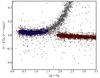 |
Fig. 6 Comparison of KiDS r-band GAaP photometry to Gaia DR1 G-band and SDSS DR9 r-band photometry. Stars with dereddened g − i colours, based on colour-calibrated KiDS GAaP data (x-axis), between 0.2 and 1.5 are selected to iteratively derive the median photometric offsets (r − G)0 (left sequence) and (r − rSDSS) (right sequence). The latter sequence of data points is shifted by 1.6 mag in (g − i)0 for clarity. The red and green outlines show the regions encompassing the data points used in the final iteration of each fit. |
The first data release of Gaia (Gaia DR1, Gaia Collaboration 2016) provides a photometrically stable and accurate catalogue (van Leeuwen et al. 2017) to which both the KiDS-North and KiDS-South fields can be compared, thus allowing a validation of the photometric homogeneity over the full survey. The photometry released in Gaia DR1 is based on one very broad “white light” filter, G, that encompasses the KiDS gri filters (Jordi et al. 2010), allowing photometric comparisons. For this purpose, the DR3 multi-band catalogue was matched to the Gaia DR1 catalogue, as well as the SDSS DR9 photometric catalogue, yielding between 1000 and 5000 matched point-like sources per KiDS survey tile. Since the r-band data is the highest quality in KiDS and also used for the absolute calibration, this was also our choice for a direct comparison to the G-band. Although the central wavelengths of KiDS r-band and Gaia G-band are similar, the difference in wavelength coverage does lead to a difference in the attenuation due to foreground extinction. To assess this, quadratic fits of the stellar locus in G0 − r0 vs. (g − i)0 were performed, using extinction corrected SDSS photometry for stars with 0.6 < (g − i)0< 1.6. Solving for the extinction in G in four iterations, we find a relative attenuation AG/Ar = 0.93 ± 0.01, meaning that the extinction in G is very close to that in r-band. Considering the small reddening in the KiDS fields, which is at most E(B − V) ~ 0.1 but much smaller almost everywhere in the survey area, the effect of this difference is always less than 0.01.
Subsequently we move to using KiDS data, comparing the r-band GAaP to both Gaia G measurements and to SDSS r-band PSF magnitudes. Stars with 0.2 < (g − i)GAaP< 1.5, colour-calibrated and extinction corrected, are selected and the median offset between rGAaP and G and between rGAaP and rSDSS are iteratively determined in a box of width ±0.05 mag, as illustrated in Figure 6. Extinction corrections are applied for each star, based on Schlegel et al. (1998) and the value of AG derived above. We consistently find an offset between (rGAaP − G) and rGAaP − rSDSS of 0.049 with a scatter of only 0.01 mag. This allows an indirect derivation via the Gaia data of the offset between the GAaP r-band photometry and SDSS even in the absence of SDSS data, such as in the KiDS-S field.
Following this strategy, the absolute calibration of the GAaP r-band photometry has been verified for all tiles in KiDS-ESO-DR3. Figure 7 shows the photometric offsets between rGAaP − G for the full data set both before and after applying the photometric homogenization based on overlap photometry. Table 7 summarizes the statistics of this comparison. For KiDS-North the overall picture is the same as for the direct comparison to SDSS (Fig. 4). Also in KiDS-South the homogenization works as expected, although one weakness of the current strategy is clearly revealed. The tile KIDS_350.8_-30.2 turns out to show a large photometric offset in r-band, but unfortunately was selected as a photometric anchor according to the criteria listed in Sect. 2.5. As a result this offset persists after the homogenization, and also has a detrimental effect on a neighbouring tile. This is reflected in the standard deviation of the offsets in KiDS-South, which is not significantly improved by the homogenization. From this analysis, the average offset between KiDS r-band and SDSS r-band is shown to be approximately − 0.015, which can be largely attributed to the colour term in rKiDS − rSDSS that is apparent from the tilt in the sequence of red points in Fig. 6.
The comparison with the Gaia DR1 G-band photometry shows the tremendous value of this all-sky, stable photometric catalogue for the validation, and possibly calibration, of ground-based surveys such as KiDS. Since KiDS-ESO-DR3 was released before these data became available, they are only used as a validation for the photometric calibration. However, in case of the shear catalogue described in Sect. 3.2 we provide per-tile photometric offsets in the catalogue itself that allow the photometry to be homogenized based on the comparison with Gaia G data. We are currently studying the possibilities for using Gaia data to further improve the photometric calibration of the KiDS photometry for future data releases. Although the Gaia DR1 catalogue still contains areas that are too sparse to use for our astrometric calibration, we anticipate moving from 2MASS (Skrutskie et al. 2006) to Gaia as astrometric reference catalogue once Gaia DR2 becomes available.
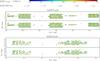 |
Fig. 7 Comparison of KiDS r-band to Gaia G-band photometry as function of position on the sky. The per-tile median photometric offset (rGAaP − G) is indicated by the colour scale, while the marker size corresponds to the mean seeing in the KiDS r-band image. Top: comparison for KiDS-North, with in the top and bottom subpanels showing the offsets before and after applying the photometric homogenization, respectively. Bottom: same as the top panel, but now for KiDS-South. |
Comparison of r-band GAaP and Gaia DR1 photometry.
3. Weak lensing shear data
For the weak gravitational analyses of KiDS accurate shear estimates of small and faint galaxy images are measured from the r-band data. This imposes especially strict requirements on the quality of the astrometric calibration (Miller et al. 2013). Furthermore, because weak lensing measurements are intrinsically noise-dominated and rely on ensemble averaging, small systematic shape residuals can significantly affect the final results. For this reason, shears are measured based on a joint fit to single exposures rather than on image stacks, avoiding any systematics introduced by re-sampling and stacking of the image pixels. Therefore, a dedicated pipeline that has already been successfully used for weak lensing analyses in previous major Wide-Field-Imaging surveys (e.g. Heymans et al. 2012; Erben et al. 2013; Hildebrandt et al. 2016) is employed to obtain optimal shape measurements from the r-band data. This dedicated pipeline makes use of THELI (Erben et al. 2005; Schirmer 2013) and the lensfit shear measurement code (Miller et al. 2013; Fenech Conti et al. 2017). In the following subsections, the additional pixel processing and the creation of the weak lensing shear catalogue are reviewed.
3.1. Image data for weak lensing
The additional r-band data reduction was done with the THELI pipeline (Erben et al. 2005; Schirmer 2013). A detailed description of our prescription to process OmegaCAM data and a careful evaluation of the data quality will be provided in a forthcoming publication (Erben et al., in prep.). We therefore only give a very short description of essential processing steps:
-
1.
The initial data set for the THELI processing is identical to thatof DR3 and consists of all r-band data observed between the 9th ofAugust 2011 and the 4th of October 2015. The raw data is retrievedfrom the ESO archive8.
-
2.
Science data are corrected for crosstalk effects. We measure significant crosstalk between CCDs #94, #95 and #96. Each pair of these three CCDs show positive or negative crosstalk in both directions. We found that the strength of the flux transfer varies on short time-scales and we therefore determine new crosstalk coefficients for each KiDS observing block. An r-band KiDS observing block extends to about 1800 s in five consecutive exposures.
-
3.
The removal of the instrumental signature (bias subtraction, flat-fielding) is performed simultaneously on all data from a two-weeks period around each new-moon and full-moon phase. Hence, two-week periods of moon-phases define our runs (processing run in the following) for OmegaCAM data processing (see also Sect. 4 of Erben et al. 2005). We tested that the instrument configuration is stable for a particular processing run. The distinction of runs with moon phases also naturally reflects usage of certain filter combinations on the telescope (u, g and r during new-moon and i during full-moon phases).
-
4.
Photometric zeropoints are estimated for all data of a complete processing run. They are obtained by calibration of all science images in a run which overlap with the Data Release 12 of the SDSS (see Alam et al. 2015). We have between 30 and 150 such images with good airmass coverage for each processing run. We note that we did not carry out extensive tests on the quality of our photometric calibration. As all required photometric analysis within weak lensing projects is performed with the DR3 data set, a rough photometric calibration of the THELI data is sufficient for our purposes.
-
5.
As a last step of the run processing we subtract the sky from all individual chips. These data form the basis for the later object shape analysis – see Hildebrandt et al. (2017) and Sect. 3.2.
-
6.
Since the astrometric calibration is particularly crucial for an accurate shear estimate of small and faint galaxy images, great care was taken in this part of the analysis and we used all available information to obtain optimal results. The available KiDS tiles were divided into five patches, three in KiDS-North and two in KiDS-South, centred around large contiguous areas. We simultaneously astrometrically calibrate all data from a given patch, i.e., we perform a patch-wide global astrometric calibration of the data. This allows us to take into account information from overlap areas of individual KiDS tiles. For the northern patches and their southern counterparts our processing differed depending on the availability of additional external data:
-
(a)
for the northern KiDS patches we use accurate astrometricreference sources from the SDSS-Data Release 12 (Alamet al. 2015) for the absoluteastrometric reference frame. No additional external data wereavailable here;
-
(b)
the southern KiDS-patches do not overlap with the SDSS, and we have to use the less accurate 2MASS catalogue (see Skrutskie et al. 2006) for the absolute astrometric reference frame. However, the area of these patches is covered by the public VST ATLAS Survey (Shanks et al. 2015). ATLAS is significantly shallower than KiDS (each ATLAS pointing consists of two 45 s OmegaCAM exposures) but it covers the area with a different pointing footprint than KiDS. This allows us to constrain optical distortions better, and to compensate for the less accurate astrometric 2MASS catalogue. Our global patch-wide astrometric calibration includes all KiDS and ATLAS r-band images covering the corresponding area.
-
7.
The astrometrically calibrated data are co-added witha weighted mean approach (see Erbenet al. 2005). The identi-fication of pixels that should not contribute and pixelweighting of usable regions is done as described in Erbenet al. (2009, 2013)for data from the Canada-France-Hawaii Telescope LegacySurvey. The set of images entering the co-addition is identi-cal to the set used for the KiDS DR1, DR2 and DR3 coadds.The final products of the THELI processing are the single-chip data (used for shear measurements, see above), the co-added science image (used for source detection), a corre-sponding weight map and a sum image (for a more detaileddescription of these products see also Erbenet al. 2013).
3.2. Weak lensing catalogue
In addition to the KiDS-ESO-DR3 catalogues we also release the catalogue that was used for the KiDS-450 cosmic shear project (Hildebrandt et al. 2017). This catalogue differs in some aspects from the DR3 catalogues as described in the following:
-
The KiDS r-band data have been reduced with an independent datareduction pipeline, THELI (Erbenet al. 2005) that is optimized forweak lensing applications. See Sect. 3.1, as well asHildebrandt et al. (2017) andKuijken et al. (2015) for details.
-
Source detection is performed on stacks reduced with THELI (see Sect. 3.1). Hence, the source lists are slightly different from the DR3 catalogues.
-
Multi-colour photometry and photo-z are estimated in the same way as for DR3 (Sect. 4) except that the source list is based on the THELI stacks.
-
The lensfit shear measurement code (Miller et al. 2013) is run on the individual exposures calibrated by THELI. This yields accurate ellipticity measurements and associated weights for each source.
-
Image simulations are used to calibrate the shear measurements as described in Fenech Conti et al. (2017). A multiplicative shear bias correction based on these results is included for each galaxy.
-
Masks for the weak lensing catalogue include defects detected on the THELI stacks and differ slightly from the DR3 masks. This masking information is also included in the lensing catalogues.
-
Contrary to the general purpose DR3 multi-band catalogue, the photometry is colour-calibrated, but the absolute calibration is not homogenized. Stellar locus regression was used to colour calibrate the u, g and i filters to the r-band, while no overlap photometry scheme was applied. In the catalogue now publicly available zeropoint offsets derived from Gaia DR1 photometry (Sect. 2.6) are included in the catalogue and can be used to homogenize the absolute calibration.
More details can be found in Hildebrandt et al. (2017). Descriptions of all columns in this weak lensing catalogue can be found in Appendix A.4 and Table A.6.
4. Photometric redshifts
Several sets of photometric redshifts are publicly available, based on the KiDS DR3 data set. These include photo-z’s derived using the BPZ template fitting method (Benítez 2000), as well as photo-z’s based on two different machine-learning techniques. In the following sections we discuss the various sets of photo-z’s, followed by a discussion in Sect. 4.4 of their performance and applicability to specific science cases.
The following sections describe the computation of the different sets of photo-z’s. In Sect. 4.1 the two available BPZ data sets are discussed and compared, while Sects. 4.2 and 4.3 focus on the two machine-learning based data sets. Finally, in Sect. 4.4 all photo-z sets are juxtaposed with the same spectroscopic data sets in order to provide an objective comparison between them, together with recommendations for different use cases. In all places where photometric redshifts are compared to spectroscopic redshifts, relative errors in the photo-z’s are defined as  (4)and catastrophic outliers as having | δz | > 0.15. Furthermore, σ and NMAD denote the standard deviation and the normalized median absolute deviation, the latter defined as
  (5)and reported values are always without clipping of outliers.
4.1. BPZ photometric redshifts
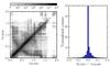 |
Fig. 8 Comparison of the BPZ photo-z’s included in the DR3 multi-band catalogue (zB,DR3) and in the KiDS-450 shear catalogue (zB,K450). Left: 2D histogram of the direct comparison. The grey scale indicating the number of sources per bin is logarithmic. Right: normalized histogram of zB,DR3 − zB,K450. |
Both the KiDS DR3 multi-band catalogue (Sect. 2), as well as the KiDS-450 weak lensing shear catalogue (Sect. 3.2), include photometric redshifts based on the Bayesian template fitting photo-z code pioneered by Benítez (2000). These photo-z’s are calculated following the methods developed for CFHTLenS (Heymans et al. 2012; Hildebrandt et al. 2012), making use of the re-calibrated templates from Capak (2004). A more detailed description of the procedures applied specifically to the KiDS data can be found in Kuijken et al. (2015). Included in the DR3 catalogue (see Table A.2) are the best-fit photometric redshift zB and the best-fit spectral type. Since the spectral types are interpolated, the best-fit value does not necessarily correspond to one type, but can be fractional. The catalogue also includes the ODDS parameter, which is a measure of the uni-modality of the redshift probability distribution function (PDF) and can be used as a quality indicator. Not included in the catalogue are the posterior redshift PDFs, which are available for download from the DR3 website9. The KiDS-450 shear catalogue also provides zB, ODDS and the best-fit template, but additionally also the lower and upper bounds of the 95% confidence interval of zB (see Table A.6).
Since photo-z’s critically rely on accurate colours, both sets of BPZ photo-z’s make use of GAaP photometry (Sect. 2.4), measured on the same Astro-WISE-reduced ugri coadded images from the KiDS public data releases. There are, however, some differences between the two data sets. Source detection for the DR3 multi-band catalogue is performed on the Astro-WISE-reduced r-band coadds, while for the KiDS-450 shear catalogue this is done on the THELI-reduced r-band coadds. Because the astrometry is derived independently between these reductions, there exist small (typically subpixel) offsets between the positions. The same small offsets exist between the GAaP apertures used for the two data sets, which can introduce small photometric differences. Furthermore, for KiDS-450 the GAaP ugri photometry was colour-calibrated using stellar locus regression, with no homogenization of the absolute calibration. On the other hand, for DR3 only the gri filters were colour-calibrated using stellar locus regression, while the u- and r-band absolute calibration were independently homogenized (Sect. 2.5). Although the absolute calibration of the photometry affects the BPZ priors, this is not expected to have a major effect on the redshift estimates. There might be some small effect from the difference in the calibration of the u-band between the two data sets. Finally, the KiDS-450 shear catalogue is limited to relatively faint sources with 20 <r< 25.
A direct comparison between the two BPZ photo-z sets is shown in the left panel of Fig. 8. The vast majority of sources lie along the diagonal, with almost mirror symmetric low-level structure visible on either side. The normalized histogram of the differences between the two sets of photo-z’s (right panel of Fig. 8) shows a narrow peak centred at 0. The photo-z resolution is 0.01 and 49% of the sources have the same best photo-z estimate, zB, both in the DR3 and in the KiDS-450 data set; 65% of all sources have values of zB that agree within 0.01 and 93% within 0.1. To verify the assumption that the lack of homogenization of the absolute r-band calibration in KiDS-450 does not significantly affect the photo-z results, these same comparisons were done limited to the tiles with derived zeropoint offsets larger than 0.1 mag. For this set of 15 tiles the results are very similar, with 45% of sources having identical photo-z and 64% and 93% agreeing to within 0.01 and 0.1, respectively, confirming that the absolute calibration does not have a substantial effect.
There are no signs of significant biases or trends between the two sets of BPZ photo-z’s, and we conclude that the two BPZ based sets of photo-z’s can be considered to be consistent for most intents and purposes.
4.2. MLPQNA photometric redshifts and Probability Distribution Functions
Photometric redshifts for KiDS DR3 have also been produced using the MLPQNA (Multi Layer Perceptron with Quasi Newton Algorithm) machine learning technique, following the analysis for KiDS DR2 (Cavuoti et al. 2015). This supervised neural network was already successfully employed in several photometric redshift experiments (Biviano et al. 2013; Brescia et al. 2013, 2014). The typical mechanism for a supervised machine learning method to predict photometric redshifts foresees the creation of a Knowledge Base (hereafter KB), split into a training set for the model learning phase and a blind test set for evaluating the overall performance of the model. The term “supervised” implies that both training and test sets must contain objects for which the spectroscopic redshift, e.g. the ground truth, is provided.
In the specific case of DR3, the KB used for MLPQNA is composed of 214 tiles of KiDS data cross-matched with SDSS-III data release 9 (Ahn et al. 2012) and GAMA data release 2 (Liske et al. 2015) merged spectroscopic redshifts. The photometry is based on the ugri homogenized magnitudes, based on the GAaP measurements (hereafter mag_gaap bands), two aperture magnitudes, measured within circular apertures of 4′′ and 6′′ diameter, respectively, corrected for extinction and zeropoint offsets, and related colours, for a total of 21 photometric parameters for each object. The initial combination of the tiles leads to 120 047 objects, after which the tails of the magnitude distributions and sources with missing magnitude measurements were removed.
Two separate experiments were performed, within different zspec ranges: i) 0.01 ≤ zspec ≤ 1 and ii) 0.01 ≤ zspec ≤ 3.5. After cleaning we subdivided the data into training and test sets. For experiment i) we obtained 66 731 objects for training and 16 742 test objects and for experiment ii) 70 688 training objects and 17 659 test objects. Scatter plots for the two experiments are shown, respectively, in the left and middle panels of Fig. 9.
The statistics, calculated for the quantity δz (Eq. (4)), obtained for experiment i) are mean δz = 0.0014, σ = 0.035 and NMAD (Eq. (5)) = 0.018, with 0.93% outliers (| δz | > 0.15). The distribution of residuals is shown by the blue histogram in the right panel of Fig. 9. For experiment ii) the values are the following:  , σ = 0.101 and NMAD = 0.022, with 3.4% outliers. In this case the residual distribution is shown in red in the right panel of Fig. 9.
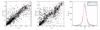 |
Fig. 9 Results of the MLPQNA photo-z experiments. Left: scatter plot of zspec vs. zphot for the experiment limiting zspec between 0.01 and 1. Centre: same as the left panel but for zspec between 0.01 and 3.5. Right: histograms of the residual distribution for the experiment with 0.01 <zspec< 1.0 (blue) and 0.01 <zspec< 3.5 (red). |
The photometric redshifts are characterized by means of a photo-z Probability Density Function (PDF), derived by the METAPHOR (Machine-learning Estimation Tool for Accurate PHOtometric Redshifts) method, designed to provide a reliable PDF of the error distribution for empirical models (Cavuoti et al. 2017). The method is implemented as a modular workflow, whose internal engine for photo-z estimation makes use of the MLPQNA neural network. The METAPHOR pipeline is based on three functional macro phases:
-
data Pre-processing: data preparation, photometric evaluationand error estimation of the KB, followed by its perturbation;
-
photo-z prediction: training/test phase performed through the MLPQNA model;
-
PDF estimation: production of the photo-z’s PDF and evaluation of the statistical performance.
Given the spectroscopic sample, randomly shuffled and split into training and test sets, we proceed by training the MLPQNA model and by perturbing the photometry of the given test set to obtain an arbitrary number N test sets with a variable photometric noise contamination. Then we submit the N + 1 test sets (i.e. N perturbed sets plus the original one) to the trained model, thus obtaining N + 1 estimates of photo-z. With these N + 1 values we perform a binning in photo-z, thus calculating for each one the probability that a given photo-z value belongs to each bin. We selected a binning step of 0.01 for the described experiments.
The photometry perturbation can be selected among a series of types, described in Cavuoti et al. (2017). Here the choice is based on the following expression, which is applied to the given j magnitudes of each band i as many times as the number of perturbations of the test set:  (6)where αi is a multiplicative constant, defined by the user and Fij is a band-specific bimodal function designed to realistically scale the contribution of Gaussian noise to the magnitudes. To this end, for each magnitude Fij takes the maximum of a constant, heuristically chosen for each band, or a polynomial fit to the magnitude-binned photometric errors; in other words, at the faint end Fij follows the derived photometric uncertainties and at the bright end it has a user-defined constant value. Finally, the term u(μ = 0,σ = 1) in Eq. (6)is randomly drawn from a Gaussian centred on 0 with unit variance. A detailed description of the produced photo-z catalogue will be provided in Amaro et al. (in prep.).
The final photo-z catalogue produced consists of 8 586 152 objects, by including all data compliant with the magnitude ranges imposed by the KB used to train our model and specified in Appendix A.3. For convenience, the whole catalogue was split into two categories of files, namely a single catalogue file with the best predicted redshifts for the KiDS DR3 multi-band catalogue, and a set of 440 files, one for each included survey tile, that contain the photo-z PDFs. The file formats are specified in Tables A.3 and A.4.
4.3. ANNz2 photometric redshifts
Photometric redshifts based on another machine learning method, namely ANNz2 (Sadeh et al. 2016), are provided for KiDS DR3 as well. This versatile tool combines various ML approaches (artificial neural networks, boosted decision trees, etc.) and allows the user to derive photometric redshifts and their PDFs based on spectroscopic training sets. It also incorporates a weighting scheme, using a kd-tree algorithm, which enables weighting the training set to mimic the photometric properties of the target data (see e.g. Lima et al. 2008). A similar principle has been applied in the KiDS cosmic shear analysis by Hildebrandt et al. (2017) to directly calibrate photometric redshift distributions based on deep spectroscopic data. Here we use a similar set of redshift samples as in Hildebrandt et al. (2017) for the training, including fields outside of the main KiDS footprint, which were purposely observed for the survey, namely: a non-public extension of zCOSMOS data (Lilly et al. 2009), kindly shared by the zCOSMOS team; an ESO-released10 compilation of spec-z’s in the CDFS field; as well as redshift data from two DEEP2 fields (Newman et al. 2013). This is supplemented by redshift samples not used by Hildebrandt et al. (2017), i.e. GAMA-II data11 (Liske et al. 2015); 2dFLenS measurements (Blake et al. 2016); SDSS-DR13 galaxy spectroscopy (SDSS Collaboration et al. 2016); additional redshifts in the COSMOS field from the “GAMA G10” analysis (Davies et al. 2015); and extra redshifts in the CDFS field from the ACES survey (Cooper et al. 2012). After combining all these datasets and removing duplicates we have over 300 000 sources detected also by KiDS that are used for training and tests of the photometric redshift accuracy. We note however that the bulk of these (~200 000) come from GAMA which provides information only at r< 19.8. It is the availability of the deep spectroscopic data covered by KiDS imaging that allows us to derive machine-learning photo-z’s at almost the full depth of the photometric sample. The details of the methodology and photo-z statistics will be provided in Bilicki et al. (in prep.). Here we report the main results of our experiments, and compare them with the fiducial KiDS photo-z’s available from BPZ.
The full KiDS spectroscopic sample is currently dominated by relatively low-redshift ( ) and bright galaxies. By splitting it randomly into training and test sets we were thus able to test the performance of ANNz2 for KiDS in this regime. The experiments indicate better results for ANNz2 than for BPZ at these low redshifts: mean bias of δz equal to 0.0015, with σ = 0.068 and NMAD = 0.025 and 3.3% outliers as compared to
  , σ = 0.086, NMAD = 0.035 and 3.9% outliers for the same sources from BPZ.
A more relevant test in view of future applications of the KiDS machine-learning photo-z’s at the full depth of the survey is by selecting deep spectroscopic samples for tests. For this purpose we used the COSMOS-KiDS ( ) and CDFS-KiDS (
 ) data as two independent test sets by training ANNz2 on spectroscopic data with each of them removed in turn (i.e. training on data without COSMOS and testing on COSMOS, and similarly for CDFS). We note that these tests might be prone to cosmic variance as the two datasets cover only one KiDS tile each and include just ~17 000 and ~5 500 spectroscopic sources, respectively. In this procedure we adopted the aforementioned weighting of the training data, as implemented in the ANNz2 code. We compare the results of these experiments to BPZ, which does not depend on a training set. In this case the results point to comparable performance of ANNz2 and BPZ, although the former seems to be less biased overall. For the COSMOS data used as the independent test set, we obtained
  , σ = 0.164, NMAD = 0.077 and 20.8% outliers for ANNz2 (cf.
  , σ = 0.173, NMAD = 0.078, and 21.3% outliers for BPZ), and when CDFS was used in the same way, we found
  , σ = 0.194, NMAD = 0.096 and 25.7% outliers for ANNz2 (cf.
  , σ = 0.181, NMAD = 0.082, and 23.4% outliers for BPZ). Figure 10 compares the relative error δz of ANNz2 and BPZ in the CDFS test field, indicating that the two methods exhibit different types of systematics.
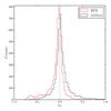 |
Fig. 10 Comparison of normalised photometric redshift errors for ANNz2 (black) and BPZ (red) in the CDFS field. |
We make available a catalogue of photometric redshifts derived with the ANNz2 method for all the DR3 sources that have valid GAaP magnitudes in all four bands. Table A.5 lists the included columns. This includes almost 39.2 million sources, which is 80% of the full DR3 multi-band dataset. However, for scientific applications only part of these data will be useful and the catalogue needs to be purified of artefacts (using appropriate flags), stellar sources, as well as sources of unreliable photometry. In addition, the full catalogue is deeper photometrically than the spectroscopic training set, so to avoid often unreliable extrapolation, the data should be preferentially limited to the depth of the spectroscopic calibration sample. Leaving the particular selections to the user, we provide however a “fiducial” selection for scientific use, marked with a binary flag. The applied selection criteria, specified in detail in Appendix A.3, remove sources affected by artifacts, classified as stars, as well as sources fainter than the photometry of the spectroscopic sample. The latter criteria are used in order to avoid extrapolation beyond what is available in training, since sources fainter than any of this limits may have unreliable ANNz2 photo-z’s and should be used with care. These selections altogether yield approximately 20.5 million sources in the fiducial sample.
4.4. Discussion
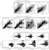 |
Fig. 11 Comparison of photometric redshifts to spectroscopic redshifts. Top: direct comparisons of best-guess photo-z’s against GAMA DR2 spec-z’s. From left to right the panels show the BPZ photo-z’s in the DR3 multi-band catalogue, the MLPQNA photo-z’s and the ANNz2 photo-z’s. The red dashed line corresponds to zB = zspec and the contours are chosen randomly to enhance the clarity of the figures. Centre: same as the top row, but now comparing to zCOSMOS bright DR3 spec-z’s and with on the left a panel added for the BPZ photo-z’s included in the KiDS-450 shear catalogue. Bottom: normalized photo-z error δz versus r-band magnitude. The panels in the first row show the comparison to GAMA DR2 and the second row the comparison to zCOSMOS bright DR3. The order of the panels follows the order in the top and centre rows. |
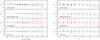 |
Fig. 12 Trends in photometric redshift bias. Left: the mean normalized photo-z error δz is plotted in bins of r-band magnitude for each of the photo-z sets. Dashed lines correspond to the comparison with the GAMA DR2 spec-z and the dotted lines to the comparison with the zCOSMOS bright DR3 spec-z, where the latter have been offset along the x-axis slightly to improve clarity. Error bars show the standard deviation in δz. Right: same as the left panel, but now δz for bins of zspec. |
Due to the different methods to compute the photo-z sets described above, including different training sets for the two machine learning methods, an objective comparison and quality assessment is warranted. For this purpose we juxtapose each catalogue with two publicly available spectroscopic data sets that overlap with the KiDS-ESO-DR3 area and provide accurate redshifts in different redshift ranges. The second data release of GAMA (Liske et al. 2015) contains spectroscopic redshifts for over 70 000 galaxies in three 48 square degree fields overlapping with KiDS-North. GAMA DR2 is complete to an r-band Petrosian magnitude of ~19, and probes redshifts up to ~0.4. The best available secure redshift estimates were obtained from the SpecObj table, resulting in values for 70 026 sources, of which 76% come from GAMA spectroscopy, 18% from SDSS/BOSS DR10 (Ahn et al. 2014), 5% from 2dFGRS (Colless et al. 2001) and the remainder from a number of other surveys. The COSMOS field is included in the KiDS main survey area because of the availability of several deep photometric and spectroscopic data sets, and particularly for the purpose of photometric redshift validation and calibration. It should be noted that only one KiDS tile (KIDS_150.2_2.2) overlaps with the COSMOS field. We use the third data release from the zCOSMOS (Lilly et al. 2007) bright spectroscopic sample. From the spectroscopic catalogue we select reliable redshifts, based on both spectroscopic and photometric information as indicated in the zCOSMOS DR3 release notes, yielding a set of 17 890 spec-z’s.
Associating the GAMA DR2 catalogue with the DR3 BPZ, MLPQNA and ANNz2 photo-z’s yields approximately 53 000 matches, selecting only sources classified as galaxies in the DR3 multi-band catalogue (SG2DPHOT= 0) and not masked in r-band (IMAFLAGS_ISO_R= 0). The bright cut-off of r> 20 in the KiDS-450 shear catalogue prevents association to the GAMA data. The upper row of panels in Fig. 11 shows the direct comparison of the photo-z’s and the GAMA DR2 spec-z’s, while δz (Eq. (4)) is plotted against r-band magnitude in the third row of panels. Associating the KiDS photo-z catalogues to the zCOSMOS spec-z’s gives of order 10 000 matches (Table 8) for unmasked galaxies12. The second row of panels in Fig. 11 shows the direct comparison between the photo-z’s and the spec-z’s, and δz is plotted against r-band magnitude in the bottom row of panels13. Statistical measures of the photo-z biases, scatter and outlier rates are again tabulated in Table 8 and Fig. 12 shows the trends and scatter in the photo-z bias as function of r-band magnitude and spec-z.
In the magnitude/redshift regime probed by the GAMA DR2 data the scatter and outlier rates are very similar between the three data sets, but the machine learning methods yield significantly smaller photo-z bias:  for BPZ versus 0.002 and 0.003 for MLPQNA and ANNz2, respectively (Table 8). However, the direct comparison between the ANNz2 and the GAMA DR2 data (top right panel, Fig. 11), as well as the trend versus zspec (bottom right panel in Fig. 12), show a trend in the bias going from 0 <zspec< 0.4.
As expected, for the much fainter and consequently noisier sources probed by the zCOSMOS bright DR3 data, the photo-z quality deteriorates in all aspects, showing higher bias, scatter and outlier rates (see Table 8). The two sets of BPZ photo-z’s show very similar behaviour. Also in this fainter sample, there is a clear bias present in the BPZ photo-z’s, but this time negative,  and − 0.040. Both for the GAMA and the zCOSMOS comparison the δz vs. r plots for BPZ show a slightly tilted sequence. This small magnitude dependence in the bias is confirmed by the trends visible in Fig. 11. Furthermore, in the direct comparison of both BPZ data sets to zCOSMOS a sequence of points can be seen along zphot,BPZ = 0.2 extending to higher spec-z. This is consistent with the bias found by Hildebrandt et al. (2017) in their lowest redshift bin (0.1 <z< 0.3). The quality of the ANNz2 results is similar to that of BPZ with a bias of comparable amplitude, albeit with opposite sign (
 ), and similar NMAD and outlier rate. However, the MLPQNA results are significantly degraded, particularly for sources with r> 20.5, where both the bias and the scatter show a clear jump (Fig. 12, left). This is presumably caused by the knowledge base used for training the network, which is based on SDSS and GAMA and does not extend to these faint magnitudes. Nevertheless, even with the inclusion of deeper spectroscopic data in the knowledge base used for the ANNz2 data set, this comparison indicates that the BPZ results are certainly competitive with machine learning in this domain. However, it should be kept in mind that the fact that this particular comparison is based on a single 1 deg2 field limits its statistical power and renders it prone to cosmic variance.
Which set of photo-z’s is preferred will depend on the scientific use case. For relatively bright and nearby galaxies (r< 20.5; z< 0.5) the MLPQNA catalogue provides the most reliable redshifts. Moving to fainter sources the BPZ and ANNz2 results are strongly preferred, but caution has to be observed regarding biases that can be dependent on magnitude or redshift.
KiDS photo-z quality.
5. Data access
There are several ways through which KiDS-ESO-DR3 and associated data products can be accessed. An overview is presented in this section and up-to-date information is also available at the KiDS DR3 website.
5.1. KiDS-ESO-DR3 main release
The data products that constitute the main DR3 release (stacked images, weight and flag maps, and single-band source lists for 292 survey tiles, as well as a multi-band catalogue for the combined DR1, DR2 and DR3 survey area of 440 survey tiles, see Sect. 2) are released via the ESO Science Archive, and also accessible via Astro-WISE and the KiDS website.
5.1.1. ESO Science Archive
All main release data products are disseminated through the ESO Science Archive Facility14, which provides several interfaces and query forms. All image stacks, weight maps, flag maps and single-band source lists are provided on a per tile basis via the “Phase 3 main query form”. This interface supports queries on several parameters, including position, object name, filter, observation date, etc. and allows download of the tile-based data files. Also the multi-band catalogue, which is stored in per-tile data files, is available in this manner. A more advanced method to query the multi-band catalogue is provided by the “Catalogue Facility query interface”, which enables users to perform queries on any of the catalogue columns, for example facilitating selections based on area, magnitude, photo-z or shape information. Query results can subsequently be exported to various (single-file) formats.
5.1.2. Astro-WISE archive
The data products can also be retrieved from the Astro-WISE system (Begeman et al. 2013). This data processing and management system is used for the production of these data products and retains the full data lineage. For scientists interested in access to various quality controls, further analysis tools, or reprocessing of data this access route may be convenient. The DBviewer web service15 allows querying for data products and supports file downloads, viewing of inspection plots, and data lineage browsing. Links with DBviewer queries to complete sets of data products are compiled on the KiDS DR3 website.
5.1.3. KiDS DR3 website
Apart from offering an up-to-date overview of all data access routes, the KiDS DR3 website16 also provides alternative ways for data retrieval and quality control.
The synoptic table presents for each observation (tile/filter) a combination of inspection plots relating to the image and source extraction quality, as well as links for direct downloads of the various data FITS files. Furthermore, direct batch downloads of all DR3 FITS files are supported by supplying wget input files.
5.2. Machine-learning photometric redshifts
Two sets of photometric redshifts derived using machine-learning techniques are released. Both the MLPQNA (Sect. 4.2) photo-z data set, which includes PDFs, and the ANNz2 (Sect. 4.3) data set are available for download solely via the KiDS DR3 website17.
5.3. Lensing shear data
The lensing shear catalogue that was used by Hildebrandt et al. (2017) (Sect. 3.2) is released both through ESO and CADC. At the ESO Science Archive Facility the “Catalog Facility query interface” supports queries on catalogue columns or on position, after which the output can be exported or viewed, while the “Phase 3 main query form” allows the (per tile) FITS files to be retrieved. At CADC this weak lensing catalogue can be accessed through a web form18, that allows a custom selection of columns as well as filtering for any of the quantities provided in the catalogue. Via the “Graphical Search Tool” the r-band image stacks from the lensing optimized THELI reduction, as well as the weight, sum and flag images (see Sect. 3.1) can be retrieved. The single-exposure frames are available on request from the authors.
Finally, batch download of the catalogue FITS files is also possible from the KiDS DR3 website.
6. Summary and outlook
The Kilo-Degree Survey (KiDS, de Jong et al. 2013) is an ESO Public Survey at the VLT Survey Telescope (VST) that aims to map 1500 square degrees of extra-galactic sky in four broad-band filters (ugri). Together with its sister survey VIKING (Edge et al. 2013), this will result in a 9-band optical-infrared data set with excellent depth and image quality. While KiDS was designed as a tomographic weak lensing survey, the data allow for a variety of scientific analyses, ranging from cosmology, and rare object discovery to the study of Milky Way structure.
The third data release of KiDS (Sect. 2) adds 292 survey tiles to the previously released 148 tiles. Released data products include astrometrically and photometrically calibrated stacked images, weight maps, flag maps and single-band source lists for the 292 new tiles, and a multi-band catalogue for the combined 440 survey tiles of KiDS DR1, DR2 and DR3 (Sect. 2.1). This catalogue for the first time contains Gaussian Aperture and Photometry measurements (Sect. 2.4), homogenization of the photometric calibration based on Stellar Locus Regression and Overlap Photometry (Sect. 2.5) and photometric redshifts (Sect. 4.1). Cross-matching the KiDS DR3 data to Gaia DR1 (Gaia Collaboration 2016) allows an independent verification of the photometric calibration, indicating that the calibration is stable at the ≃2% level (Sect. 2.6).
Also made publicly available are a number of associated data products. Accurate galaxy ellipticities are provided in a weak lensing shear catalogue (Sect. 3.2), which was used for the first cosmic shear measurements with KiDS data (Hildebrandt et al. 2017). The shear measurements are based on lensing-optimized single-exposure r-band images (Sect. 3.1). Photometric redshifts derived using two different Machine Learning techniques, namely Multi Layer Perceptron with Quasi Newton Algorithm (Sect. 4.2) and ANNz2 (Sect. 4.3), which particularly at z< 0.5 provides more accurate redshifts than the template-fitting redshifts included in the main DR3 catalogue (see Sect. 4.4).
Looking forward to the fourth data release of KiDS, we anticipate a number of important new developments. Improved accuracy and stability of the photometry is foreseen, as an improved calibration strategy that makes use of the Gaia data is actively pursued. Furthermore, combining the optical KiDS data with the near-infrared VIKING data is nearing completion, which will allow better constrained photometric redshifts at z> 1. Recently the observational progress has improved significantly. DR4 is expected to increase the total number of released survey tiles by approximately 250, while based on the current data rates, completion of the full survey is anticipated during the course of 2019.
Constant to 0.2% or better for g, r and i (Verdoes Kleijn et al. 2013; de Jong et al. 2015).
This information is also available in the tile table on the DR3 website (http://kids.strw.leidenuniv.nl/DR3).
Selected here with CLASS_STAR > 0.8.
See the OmegaCAM news page for more details: https://www.eso.org/sci/facilities/paranal/instruments/omegacam/news.html
At the relatively high Galactic latitudes where the KiDS survey areas are located the full dust path is probed at distances between 0.5 and 1.0 kpc (Green et al. 2015). Given the r-band brightness limit of r ~ 16 this implies that 90% of the stars probed by KiDS are behind practically all the obscuring dust.
Since the KiDS-450 catalogue is already filtered to include only unmasked galaxies, no additional filtering is applied during this association.
The zCOSMOS bright sample is magnitude limited at IAB = 22.5, but the included sources extend to ~24 in r-band GAaP magnitudes, which are not total magnitudes.
Acknowledgments
We thank Léon Koopmans for insightful comments and feedback.
Based on data products from observations made with ESO Telescopes at the La Silla Paranal Observatory under programme IDs 177.A-3016, 177.A-3017 and 177.A-3018, and on data products produced by Target/OmegaCEN, INAF-OACN, INAF-OAPD and the KiDS production team, on behalf of the KiDS consortium. OmegaCEN and the KiDS production team acknowledge support by NOVA and NWO-M grants. Members of INAF-OAPD and INAF-OACN also acknowledge the support from the Department of Physics & Astronomy of the University of Padova, and of the Department of Physics of Univ. Federico II (Naples). This work is supported by the Deutsche Forschungsgemeinschaft in the framework of the TR33 “The Dark Universe”. The research leading to these results has received funding from the People Programme (Marie Curie Actions) of the European Union’s Seventh Framework Programme (FP7/2007-2013) under REA grant agreement number 627288. GAMA is a joint European-Australasian project based around a spectroscopic campaign using the Anglo-Australian Telescope. The GAMA input catalogue is based on data taken from the Sloan Digital Sky Survey and the UKIRT Infrared Deep Sky Survey. Complementary imaging of the GAMA regions is being obtained by a number of independent survey programmes including GALEX MIS, VST KiDS, VISTA VIKING, WISE, Herschel-ATLAS, GMRT and ASKAP providing UV to radio coverage. GAMA is funded by the STFC (UK), the ARC (Australia), the AAO, and the participating institutions. The GAMA website is http://www.gama-survey.org/. Based on zCOSMOS observations carried out using the Very Large Telescope at the ESO Paranal Observatory under Programme ID: LP175.A-08392. dFLenS is based on data acquired through the Australian Astronomical Observatory, under program A/2014B/008.
J.T.A.d.J. is supported by the Netherlands Organisation for Scientific Research (NWO) through grant 614.061.610. G.V.K. acknowledges financial support from The Netherlands Research School for Astronomy (NOVA) and Target. Target is supported by Samenwerkingsverband Noord Nederland, European fund for regional development, Dutch Ministry of economic affairs, Pieken in de Delta, Provinces of Groningen and Drenthe. H.Hi. is supported by an Emmy Noether grant (No. Hi 1495/2-1) of the Deutsche Forschungsgemeinschaft. K.K. acknowledges support by the Alexander von Humboldt Foundation. M.Br. acknowledges financial contribution from the agreement ASI/INAF I/023/12/1. M.Bi. is supported by the Netherlands Organization for Scientific Research, NWO, through grant number 614.001.451, and by the European Research Council through FP7 grant number 279396. R.N. acknowledges support from the German Federal Ministry for Economic Affairs and Energy (BMWi) provided via DLR under project No. 50QE1103. C.T. is supported through an NWO-VICI grant (project number 639.043.308). C.B. acknowledges the support of the Australian Research Council through the award of a Future Fellowship. I.F.C. acknowledges the use of computational facilities procured through the European Regional Development Fund, Project ERDF-080 “A supercomputing laboratory for the University of Malta”. R.H. acknowledges support from the European Research Council FP7 grant number 279396. C.H. acknowledges support from the European Research Council under grant number 647112. H.Ho. acknowledges support from the European Research Council under FP7 grant number 279396. L.M. acknowledges support from STFC grant ST/N000919/1. M.V. acknowledges support from the European Research Council under FP7 grant number 279396 and The Netherlands Organisation for Scientific Research (NWO) through grants 614.001.103.
References
- Ahn, C. P., Alexandroff, R., Allen de Prieto, C., et al. 2012, ApJS, 203, 21 [NASA ADS] [CrossRef] [Google Scholar]
- Ahn, C. P., Alexandroff, R., Allen de Prieto, C., et al. 2014, ApJS, 211, 17 [NASA ADS] [CrossRef] [Google Scholar]
- Alam, S., Albareti, F. D., Allen de Prieto, C., et al. 2015, ApJS, 219, 12 [NASA ADS] [CrossRef] [Google Scholar]
- Begeman, K., Belikov, A. N., Boxhoorn, D. R., & Valentijn, E. A. 2013, Experim. Astron., 35, 1 [Google Scholar]
- Benítez, N. 2000, ApJ, 536, 571 [NASA ADS] [CrossRef] [Google Scholar]
- Bertin, E., & Arnouts, S. 1996, A&AS, 117, 393 [NASA ADS] [CrossRef] [EDP Sciences] [Google Scholar]
- Biviano, A., Rosati, P., Balestra, I., et al. 2013, A&A, 558, A1 [NASA ADS] [CrossRef] [EDP Sciences] [Google Scholar]
- Blake, C., Amon, A., Childress, M., et al. 2016, MNRAS, 462, 4240 [NASA ADS] [CrossRef] [Google Scholar]
- Brescia, M., Cavuoti, S., D’Abrusco, R., Longo, G., & Mercurio, A. 2013, ApJ, 772, 140 [NASA ADS] [CrossRef] [Google Scholar]
- Brescia, M., Cavuoti, S., Longo, G., & De Stefano, V. 2014, A&A, 568, A126 [NASA ADS] [CrossRef] [EDP Sciences] [Google Scholar]
- Brouwer, M. M., Cacciato, M., Dvornik, A., et al. 2016, MNRAS, 462, 4451 [NASA ADS] [CrossRef] [Google Scholar]
- Brouwer, M. M., Visser, M. R., Dvornik, A., et al. 2017, MNRAS, 466, 2547 [NASA ADS] [CrossRef] [Google Scholar]
- Capaccioli, M., Schipani, P., de Paris, G., et al. 2012, in Science from the Next Generation Imaging and Spectroscopic Surveys, ESO Meeting, 1 [Google Scholar]
- Capak, P. L. 2004, Ph.D. thesis, University of Hawai’i [Google Scholar]
- Cavuoti, S., Brescia, M., Tortora, C., et al. 2015, MNRAS, 452, 3100 [NASA ADS] [CrossRef] [Google Scholar]
- Cavuoti, S., Amaro, V., Brescia, M., et al. 2017, MNRAS, 465, 1959 [NASA ADS] [CrossRef] [Google Scholar]
- Chambers, K. C., Magnier, E. A., Metcalfe, N., et al. 2016, ArXiv e-prints [arXiv:1612.05560] [Google Scholar]
- Colless, M., Dalton, G., Maddox, S., et al. 2001, MNRAS, 328, 1039 [NASA ADS] [CrossRef] [Google Scholar]
- Cooper, M. C., Yan, R., Dickinson, M., et al. 2012, MNRAS, 425, 2116 [NASA ADS] [CrossRef] [Google Scholar]
- Davies, L. J. M., Robotham, A. S. G., Driver, S. P., et al. 2015, MNRAS, 452, 616 [NASA ADS] [CrossRef] [Google Scholar]
- de Jong, J. T. A., Verdoes Kleijn, G. A., Kuijken, K. H., & Valentijn, E. A. 2013, Exp. Astron., 35, 25 [Google Scholar]
- de Jong, J. T. A., Verdoes Kleijn, G. A., Boxhoorn, D. R., et al. 2015, A&A, 582, A62 [NASA ADS] [CrossRef] [EDP Sciences] [Google Scholar]
- Driver, S. P., Hill, D. T., Kelvin, L. S., et al. 2011, MNRAS, 413, 971 [NASA ADS] [CrossRef] [Google Scholar]
- Edge, A., Sutherland, W., Kuijken, K., et al. 2013, The Messenger, 154, 32 [NASA ADS] [Google Scholar]
- Erben, T., Schirmer, M., Dietrich, J. P., et al. 2005, Astron. Nachr., 326, 432 [NASA ADS] [CrossRef] [Google Scholar]
- Erben, T., Hildebrandt, H., Lerchster, M., et al. 2009, A&A, 493, 1197 [NASA ADS] [CrossRef] [EDP Sciences] [Google Scholar]
- Erben, T., Hildebrandt, H., Miller, L., et al. 2013, MNRAS, 433, 2545 [NASA ADS] [CrossRef] [Google Scholar]
- Fenech Conti, I., Herbonnet, R., Hoekstra, H., et al. 2017, MNRAS, 467, 1627 [NASA ADS] [Google Scholar]
- Finkbeiner, D. P., Schlafly, E. F., Schlegel, D. J., et al. 2016, ApJ, 822, 66 [NASA ADS] [CrossRef] [Google Scholar]
- Gaia Collaboration (Brown, A. G. A., et al.) 2016, A&A, 595, A2 [NASA ADS] [CrossRef] [EDP Sciences] [Google Scholar]
- Green, G. M., Schlafly, E. F., Finkbeiner, D. P., et al. 2015, ApJ, 810, 25 [NASA ADS] [CrossRef] [Google Scholar]
- Heymans, C., Van Waerbeke, L., Miller, L., et al. 2012, MNRAS, 427, 146 [NASA ADS] [CrossRef] [Google Scholar]
- Hildebrandt, H., Erben, T., Kuijken, K., et al. 2012, MNRAS, 421, 2355 [NASA ADS] [CrossRef] [Google Scholar]
- Hildebrandt, H., Choi, A., Heymans, C., et al. 2016, MNRAS, 463, 635 [NASA ADS] [CrossRef] [Google Scholar]
- Hildebrandt, H., Viola, M., Heymans, C., et al. 2017, MNRAS, 465, 1454 [Google Scholar]
- Ivezić, Ž., Lupton, R. H., Schlegel, D., et al. 2004, Astron. Nachr., 325, 583 [NASA ADS] [CrossRef] [Google Scholar]
- Jordi, C., Gebran, M., Carrasco, J. M., et al. 2010, A&A, 523, A48 [NASA ADS] [CrossRef] [EDP Sciences] [Google Scholar]
- Joudaki, S., Mead, A., Blake, C., et al. 2017, MNRAS, 471, 1259 [NASA ADS] [CrossRef] [Google Scholar]
- Kuijken, K. 2011, The Messenger, 146, 8 [NASA ADS] [Google Scholar]
- Kuijken, K., Heymans, C., Hildebrandt, H., et al. 2015, MNRAS, 454, 3500 [NASA ADS] [CrossRef] [Google Scholar]
- Lilly, S. J., Le Fèvre, O., Renzini, A., et al. 2007, ApJS, 172, 70 [NASA ADS] [CrossRef] [Google Scholar]
- Lilly, S. J., Le Brun, V., Maier, C., et al. 2009, ApJS, 184, 218 [Google Scholar]
- Lima, M., Cunha, C. E., Oyaizu, H., et al. 2008, MNRAS, 390, 118 [NASA ADS] [CrossRef] [Google Scholar]
- Liske, J., Baldry, I. K., Driver, S. P., et al. 2015, MNRAS, 452, 2087 [NASA ADS] [CrossRef] [Google Scholar]
- McFarland, J. P., Verdoes-Kleijn, G., Sikkema, G., et al. 2013, Exp. Astron., 35, 45 [NASA ADS] [CrossRef] [Google Scholar]
- Miller, L., Heymans, C., Kitching, T. D., et al. 2013, MNRAS, 429, 2858 [Google Scholar]
- Newman, J. A., Cooper, M. C., Davis, M., et al. 2013, ApJS, 208, 5 [Google Scholar]
- Radovich, M., Puddu, E., Bellagamba, F., et al. 2017, A&A, 598, A107 [NASA ADS] [CrossRef] [EDP Sciences] [Google Scholar]
- Refregier, A. 2003, MNRAS, 338, 35 [NASA ADS] [CrossRef] [Google Scholar]
- Sadeh, I., Abdalla, F. B., & Lahav, O. 2016, PASP, 128, 104502 [NASA ADS] [CrossRef] [Google Scholar]
- Schirmer, M. 2013, ApJS, 209, 21 [NASA ADS] [CrossRef] [Google Scholar]
- Schlegel, D. J., Finkbeiner, D. P., & Davis, M. 1998, ApJ, 500, 525 [NASA ADS] [CrossRef] [Google Scholar]
- SDSS Collaboration (Albareti, F. D., et al.) 2016, ApJS, submitted [arXiv:1608.02013] [Google Scholar]
- Shanks, T., Metcalfe, N., Chehade, B., et al. 2015, MNRAS, 451, 4238 [NASA ADS] [CrossRef] [Google Scholar]
- Sifón, C., Cacciato, M., Hoekstra, H., et al. 2015, MNRAS, 454, 3938 [NASA ADS] [CrossRef] [Google Scholar]
- Skrutskie, M. F., Cutri, R. M., Stiening, R., et al. 2006, AJ, 131, 1163 [NASA ADS] [CrossRef] [Google Scholar]
- Tortora, C., La Barbera, F., Napolitano, N. R., et al. 2016, MNRAS, 457, 2845 [NASA ADS] [CrossRef] [Google Scholar]
- van Leeuwen, F., Evans, D. W., De Angeli, F., et al. 2017, A&A, 599, A32 [NASA ADS] [CrossRef] [EDP Sciences] [Google Scholar]
- van Uitert, E., Cacciato, M., Hoekstra, H., et al. 2016, MNRAS, 459, 3251 [NASA ADS] [CrossRef] [Google Scholar]
- Venemans, B. P., Verdoes Kleijn, G. A., Mwebaze, J., et al. 2015, MNRAS, 453, 2259 [NASA ADS] [CrossRef] [Google Scholar]
- Verdoes Kleijn, G. A., Kuijken, K. H., Valentijn, E. A., et al. 2013, Exp. Astron., 35, 103 [NASA ADS] [CrossRef] [Google Scholar]
- Viola, M., Cacciato, M., Brouwer, M., et al. 2015, MNRAS, 452, 3529 [CrossRef] [Google Scholar]
Appendix A: Catalogue columns
Appendix A.1: Single-band source list columns
Table A.1 lists the columns that are present in the single-band source lists provided in KiDS-ESO-DR3. In the following we provide additional information on certain columns:
-
2DPHOT:KiDS-CAT star/galaxy classification bitmap based onthe source morphology (see de Jonget al. 2015). Values are: 1 = highconfidence star candidate; 2 = unreliable source (e.g. cosmicray); 4 = star according to star/galaxy separation criteria; 0 = allother sources (e.g. including galaxies). Sources identified as starscan thus have a flag value of 1, 4 or 5.
-
IMAFLAGS_ISO:bitmap of mask flags indicating the types of masked areas that intersect with each source’s isophotes, as identified by the Pulecenella software (de Jong et al. 2015). Different flag values indicate different types of areas: 1 = readout spike; 2 = saturation core; 4 = diffraction spike; 8 = primary reflection halo; 16 = secondary reflection halo; 32 = tertiary reflection halo; 64 = bad pixel.
-
FLUX_APER_*and FLUXERR_APER_*:aperture flux measurements are included for 27 different aperture sizes. In the table only the smallest (2 pixels or 0.4′′ diameter) and the largest (200 pixels or 40′′ diameter) are listed; the label for the aperture of 28.5 pixels is FLUX_APER_28p5.
Columns provided in the single-band source lists.
Appendix A.2: Multi-band catalogue
Table A.2 lists the columns that are present in the multi-band catalogue provided in KiDS-ESO-DR3. In the following we provide additional information on certain columns:
-
SG2DPHOT:KiDS-CAT star/galaxy classification bitmap basedon the r-band source morphology (see de Jonget al. 2015). Values are: 1 = highconfidence star candidate; 2 = unreliable source (e.g. cosmicray); 4 = star according to star/galaxy separation criteria; 0 = allother sources (e.g. including galaxies). Sources identified as starscan thus have a flag value of 1, 4 or 5.
-
IMAFLAGS_ISO_<filter>:bitmap of mask flags indicating the types of masked areas that intersect with each source’s isophotes, as identified by the Pulecenella software (de Jong et al. 2015). Different flag values indicate different types of areas: 1 = readout spike; 2 = saturation core; 4 = diffraction spike; 8 = primary reflection halo; 16 = secondary reflection halo; 32 = tertiary reflection halo; 64 = bad pixel; 128 = manually masked area (tiles released in DR1 and DR2 only).
-
MAG_GAAP_<filter>:these magnitudes are based on Gaussian Aperture and Photometry measurements and are mainly intended for colour measurements, since they only probe the central regions of the source. They are not total magnitudes, except in the case of unresolved or point sources.
-
ZPT_OFFSET_<filter>:zero-point offsets for each filter based on stellar locus regression (gri) and overlap photometry (ugri) that homogenize the photometry over the survey. Please note that these offsets, as well as the extinction corrections EXT_SFD_<filter>have not been applied in the fluxes and magnitudes provided in the catalogue. These corrections should be applied as:
 (A.1)
(A.1) -
ODDS:a measure of the uni-modality of the redshift Probability Distribution Function; a higher value indicates a higher reliability of the best photo-z estimate.
-
T_B:the best-fit spectral template for each source; these values correspond to the following types, where fractional types can occur because the templates are interpolated: 1 = CWW-Ell, 2 = CWW-Sbc, 3 = CWW-Scd, 4 = CWW-Im, 5 = KIN-SB3, 6 = KIN-SB2 (Capak, 2004, Ph.D. Thesis, Univ. Hawai’i).
-
TILE_FLAG:bitmap that identifies coadds that are severely affected by image defects such as scattered light features. Masking of these features is currently not available for the imaging data released in KiDS-ESO-DR3, so data tiles flagged with this flag should be used with caution. The flag values indicate which filter is affected: 1 = u; 2 = g; 3 = r; 4 = i.
Columns provided in the multi-band catalogue.
Appendix A.3: Machine learning photometric redshifts
Appendix A.3.1: MLPQNA
The best photometric redshifts derived using the MLPQNA technique (Sect. 4.2) are provided in a single catalogue, featuring the columns listed in Table A.3. Apart from the photo-z values the only content consists of source ID information and positions that allow straightforward association with the KiDS DR3 multi-band catalogue.
Since the knowledge base used to train the network does not span the complete magnitude range of sources in the KiDS DR3 multi-band catalogue, the following magnitude cuts were applied, resulting in the final set of 8 586 152 photo-z’s. 16.84 < MAG_APER_20_U< 28.55 16.81 < MAG_APER_30_U< 28.14 16.85 < MAG_GAAP_U< 28.81 16.18 < MAG_APER_20_G< 24.45 15.86 < MAG_APER_30_G< 24.59 16.02 < MAG_GAAP_G< 24.49 15.28 < MAG_APER_20_R< 23.24 14.98 < MAG_APER_30_R< 23.30 15.15 < MAG_GAAP_R< 23.29 14.90 < MAG_APER_20_I< 22.84 14.56 < MAG_APER_30_I< 23.07 14.75 < MAG_GAAP_I< 22.96.
Also available are photo-z Probability Distribution Functions (PDFs) based on the MLPQNA technique. These are provided in separate catalogue files per DR3 survey tile, and their format is specified in Table A.4 below. Again, included data is limited to the PDF bins and source ID and position information that can be used to associate to the DR3 multi-band catalogue.
Columns in the MLPQNA photo-z catalogue.
Columns in the MLPQNA photo-z PDF catalogue.
Columns in the ANNz2 photo-z catalogue.
Appendix A.3.2: ANNz2
The best photometric redshifts derived using the ANNz2 technique (Sect. 4.3) are provided in a single catalogue, featuring the columns listed in Table A.5. Source ID information and positions allow straightforward association with the KiDS DR3 multi-band catalogue. Apart from the photo-z values, a flag column is provided that defines the “fiducial” set of reliable photo-z’s. This flag indicates the following selections (all are merged using an “and” condition):
-
(IMAFLAGS_ISO_band& 01010111) == 0 for each band(artefact masking, following Radovichet al. 2017);
-
SG2DPHOT== 0 (star removal);
-
MAGERR_GAAP_band>0 for each band (bad photometry removal);
-
MAG_GAAP_U<25.4 && MAG_GAAP_G<25.6 && MAG_GAAP_R<24.7 && MAG_GAAP_I<24.5.
The latter criteria reflect the 99.9 percentile of photometry in each the bands of the spectroscopic sample, and are applied to avoid extrapolation beyond what is available in training. In other words, sources fainter than any of these limits may have unreliable ANNz2 photo-z’s and should be used with care. These selections altogether yield approximately 20.5 million sources in the fiducial sample.
Appendix A.4: KiDS-450 shear catalogue
Table A.6 lists the columns provided in the KiDS-450 or KiDS-DR3.1 lensing shear catalogue. Masking of bright stars, satellite trails and other image defects results in an effective area of 360.3 deg2. The released catalogue has already been cleaned from unreliable sources, following the rejection strategy detailed in Hildebrandt et al. (2017). The faint limit of the catalogue is r = 25.0, at an approximate S/N of 5σ. Please note that the source ID’s in this catalogue are not always identical to those in the DR3 multi-band catalogue, due to the independent astrometric solution used for the lensing analysis.
Hildebrandt et al. (2017) found in their cosmic shear analysis that small residual c-terms (non-zero average shear) are present in the catalogue. These were subtracted per patch and per tomographic bin before computing the shear-shear correlation functions. Any science analysis for which c-terms are important should determine these from the data, using the lensfit weights to compute the averages.
For a number of columns additional information is provided:
-
KIDS_TILE:name of the KiDS survey tile in which the source islocated. Searching the ESO archive with this OBJECT name willlink to further data products for this tile.
-
THELI_NAME:name for the survey tile in the THELI pipeline; for scripting reasons the “.” and “-” characters are replaced with “p” and “m”, respectively.
-
MASK:bit mask indicating sources affected by different types of defects. Automatic and manual masks produced during data processing flag areas affected by bright stars (e.g. saturated pixels, reflection halos, diffraction and readout spikes) and other severe image defects. In the released catalogue the most strongly affected regions are already removed, leaving only sources with reliable measurements. As a result, only the bit mask values 2 (faint stellar reflection halo), 64 (u-band Astro-WISE manual mask), 128 (g-band Astro-WISE manual mask), 256 (r-band Astro-WISE manual mask) and 512 (i-band Astro-WISE manual mask) are present.
-
Flag:SExtractor extraction flag. Many sources that are flagged during source detection are removed from the catalogue based on the lensfit results because they do not provide reliable shear measurements. The flag values that are still present in the catalogue are 1 (the object has neighbors, bright and close enough to significantly bias the photometry, or bad pixels (more than 10% of the integrated area affected), 2 (the object was originally blended with another one) and 16 (objects aperture data are incomplete or corrupted).
-
SG_FLAG:star-galaxy separator based on analysis of the second and fourth order image moments of the source; 0 = star, 1 = galaxy.
-
MAG_u/g/r/i:the magnitudes are based on Gaussian Aperture and Photometry measurements and are dereddened and colour-calibrated using stellar locus regression. Note: these aperture magnitudes are mainly intended for colour measurements, since they only probe the central regions of the source. They are not total magnitudes, except in the case of unresolved or point sources.
-
MAG_LIM_u/g/r/i:local limiting magnitude, defined as the magnitude corresponding to a flux equal to the 1σ flux error.
-
ZPT_offset:the magnitudes reported in this catalogue have been colour-calibrated, but their absolute calibration has only been homogenized per survey tile, not over the full area. Based on a comparison of the r-band magnitudes with the Gaia DR1 (Gaia Collaboration 2016) we provide these additional photometric offsets that can be used to homogenize the photometry over the whole catalogue. The reported offsets are with respect to the Gaia photometry, but can be used to calibrate the photometry to the SDSS photometric system as follows:
 (A.2)Note: if used, these offsets must be applied to the magnitudes in all filters!
 -
T_B:the best-fit spectral template for each source; these values correspond to the following types, where fractional types can occur because the templates are interpolated: 1 = CWW-Ell, 2 = CWW-Sbc, 3 = CWW-Scd, 4 = CWW-Im, 5 = KIN-SB3, 6 = KIN-SB2 (Capak, 2004, Ph.D. Thesis, Univ. Hawai’i).
-
ODDS:a measure of the uni-modality of the redshift Probability Distribution Function; a higher value indicates a higher reliability of the best photo-z estimate.
-
fitclass:lensfit object class; the only classes included in the catalogue are 0 (galaxy, no issues) and –9 (large galaxy, overfills 48 pixel postage stamp size). The latter class is retained to avoid ellipticity selection bias in the brightest galaxy sample.
-
n_exposures_used:the number of r-band sub-exposures for which lensfit measured the shape of the source. Due to the dither pattern, or near tile edges, some sources are only present in a subset of the 5 sub-exposures.
-
e1or e2:lensfit shear estimators. Note: the e2component is defined relative to the RAJ2000, DECJ2000 grid; depending on the user’s definition of angles in this reference frame, the sign of e2may need to be changed.
-
PSF_e1and PSF_e1_exp[k]:model PSF ellipticities at the location of the object, in this case the real part of ϵPSF. PSF_e1_exp[k]is the PSF ellipticity in sub-exposure number k, while PSF_e1refers to the average over all exposures used.
-
m:the multiplicative shear calibration correction which should be applied in an ensemble average, rather than on a galaxy-by-galaxy basis (see Fenech Conti et al. 2017). Averaged catalogued ellipticities should be divided by 1+<m>, where the ellipticities should be weighted with the lensfit weight.
Columns provided in the weak lensing shear catalogue.
All Tables
All Figures
|
Fig. 1 Sky distribution of survey tiles released in KiDS-ESO-DR3 (green) and in the previous releases KiDS-ESO-DR1 and -DR2 (blue). The multi-band source catalogue covers the combined area (blue + green) and the full KiDS area is shown in grey. Top: KiDS-North. Bottom: KiDS-South. Black dashed lines delineate the locations of the GAMA fields; the single pointing at RA = 150°is centred at the COSMOS/CFHTLS D2 field. |
| In the text | |
|
Fig. 2 Data quality for KiDS-ESO-DR1 -DR2 and -DR3. Left: average PSF size (FWHM) distributions; centre: average PSF ellipticity distributions; right: limiting magnitude distributions (5σ AB in 2′′ aperture). The distributions are per filter: from top to bottom u, g, r, and i, respectively. The full histograms correspond to the 440 tiles included in the DR3 multi-band catalogue, while the lighter portions of the histograms correspond to fraction (148 tiles) previously released in KiDS-ESO-DR1 and -DR2. |
| In the text | |
|
Fig. 3 Photometric homogenization zeropoint offsets vs. offsets to SDSS. The offsets calculated by the photometric homogenization procedure are plotted as function of the per-tile offsets of stellar photometry between tiles in KiDS-North and SDSS DR9. Black and grey symbols show the SDSS offsets using GAaP and 10′′ aperture-corrected photometry, respectively, with the dashed lines indicating equality. The GAaP and aperture-corrected data are shifted down and up by 0.05 mag, respectively, to improve the clarity of the figure. Each subpanel corresponds to a different passband, denoted by the labels. |
| In the text | |
|
Fig. 4 Comparison of KiDS GAaP photometry before and after homogenization to SDSS DR13 for all tiles in KiDS-North as function of right ascension and declination. Top: the magnitude offsets with respect to SDSS before applying photometric homogenization are indicated by the colour scaling. The size of the circles represent the average PSF size in each coadded image. From top to bottom the panels correspond to the u, g, r, and i filters. Bottom: same as top panel, but after applying photometric homogenization. |
| In the text | |
|
Fig. 5 Comparison of KiDS 10′′ aperture-corrected photometry before and after homogenization to SDSS DR13 for all tiles in KiDS-North as function of right ascension and declination. Top: the magnitude offsets with respect to SDSS before applying photometric homogenization are indicated by the colour scaling. The size of the circles represent the average PSF size in each coadded image. From top to bottom the panels correspond to the u, g, r, and i filters. Bottom: same as top panel, but after applying photometric homogenization. |
| In the text | |
|
Fig. 6 Comparison of KiDS r-band GAaP photometry to Gaia DR1 G-band and SDSS DR9 r-band photometry. Stars with dereddened g − i colours, based on colour-calibrated KiDS GAaP data (x-axis), between 0.2 and 1.5 are selected to iteratively derive the median photometric offsets (r − G)0 (left sequence) and (r − rSDSS) (right sequence). The latter sequence of data points is shifted by 1.6 mag in (g − i)0 for clarity. The red and green outlines show the regions encompassing the data points used in the final iteration of each fit. |
| In the text | |
|
Fig. 7 Comparison of KiDS r-band to Gaia G-band photometry as function of position on the sky. The per-tile median photometric offset (rGAaP − G) is indicated by the colour scale, while the marker size corresponds to the mean seeing in the KiDS r-band image. Top: comparison for KiDS-North, with in the top and bottom subpanels showing the offsets before and after applying the photometric homogenization, respectively. Bottom: same as the top panel, but now for KiDS-South. |
| In the text | |
|
Fig. 8 Comparison of the BPZ photo-z’s included in the DR3 multi-band catalogue (zB,DR3) and in the KiDS-450 shear catalogue (zB,K450). Left: 2D histogram of the direct comparison. The grey scale indicating the number of sources per bin is logarithmic. Right: normalized histogram of zB,DR3 − zB,K450. |
| In the text | |
|
Fig. 9 Results of the MLPQNA photo-z experiments. Left: scatter plot of zspec vs. zphot for the experiment limiting zspec between 0.01 and 1. Centre: same as the left panel but for zspec between 0.01 and 3.5. Right: histograms of the residual distribution for the experiment with 0.01 <zspec< 1.0 (blue) and 0.01 <zspec< 3.5 (red). |
| In the text | |
|
Fig. 10 Comparison of normalised photometric redshift errors for ANNz2 (black) and BPZ (red) in the CDFS field. |
| In the text | |
|
Fig. 11 Comparison of photometric redshifts to spectroscopic redshifts. Top: direct comparisons of best-guess photo-z’s against GAMA DR2 spec-z’s. From left to right the panels show the BPZ photo-z’s in the DR3 multi-band catalogue, the MLPQNA photo-z’s and the ANNz2 photo-z’s. The red dashed line corresponds to zB = zspec and the contours are chosen randomly to enhance the clarity of the figures. Centre: same as the top row, but now comparing to zCOSMOS bright DR3 spec-z’s and with on the left a panel added for the BPZ photo-z’s included in the KiDS-450 shear catalogue. Bottom: normalized photo-z error δz versus r-band magnitude. The panels in the first row show the comparison to GAMA DR2 and the second row the comparison to zCOSMOS bright DR3. The order of the panels follows the order in the top and centre rows. |
| In the text | |
|
Fig. 12 Trends in photometric redshift bias. Left: the mean normalized photo-z error δz is plotted in bins of r-band magnitude for each of the photo-z sets. Dashed lines correspond to the comparison with the GAMA DR2 spec-z and the dotted lines to the comparison with the zCOSMOS bright DR3 spec-z, where the latter have been offset along the x-axis slightly to improve clarity. Error bars show the standard deviation in δz. Right: same as the left panel, but now δz for bins of zspec. |
| In the text | |
Current usage metrics show cumulative count of Article Views (full-text article views including HTML views, PDF and ePub downloads, according to the available data) and Abstracts Views on Vision4Press platform.
Data correspond to usage on the plateform after 2015. The current usage metrics is available 48-96 hours after online publication and is updated daily on week days.
Initial download of the metrics may take a while.