| Issue |
A&A
Volume 604, August 2017
|
|
|---|---|---|
| Article Number | A45 | |
| Number of page(s) | 22 | |
| Section | Interstellar and circumstellar matter | |
| DOI | https://doi.org/10.1051/0004-6361/201629937 | |
| Published online | 02 August 2017 | |
Simultaneous multi-frequency single pulse observations of pulsars
1 National Centre for Radio Astrophysics (Tata Institute for Fundamental Research), PO Bag 3, Ganeshkhind, 411007 Pune, India
e-mail: arun@ncra.tifr.res.in
;
bcj@ncra.tifr.res.in
2 Radio Astronomy Centre, NCRA-TIFR, 643001 Udhagamandalam (Ooty), India
Received: 21 October 2016
Accepted: 17 April 2017
Aims. We report on simultaneous multi-frequency single pulse observations of a sample of pulsars with previously reported, frequency dependent subpulse drift inferred from non-simultaneous and short observations. We aim to clarify if the frequency dependence is a result of multiple drift modes in these pulsars.
Methods. We performed simultaneous observations at 326.5 MHz with the Ooty Radio Telescope and at 326, 610, and 1308 MHz with the Giant Meterwave Radio Telescope for a sample of 12 pulsars, where frequency dependent single pulse behaviour was reported. The single pulse sequences were analysed with three types of fluctuation analysis techniques, namely longitude-resolved fluctuation spectrum technique, two-dimensional fluctuation spectrum technique and sliding two-dimensional fluctuation spectrum technique. The first two techniques are sensitive to average fluctuation properties of the pulses, whereas the last technique is used for examining the temporal behaviour of the pulses.
Results. We report subpulse drifting in PSR J0934−5249 for the first time. We also report pulse nulling measurements in PSRs J0934−5249, B1508+55, J1822−2256, B1845−19, and J1901−0906 for the first time. Our measurements of subpulse drifting and pulse nulling for the rest of the pulsars are consistent with previously reported values. Contrary to previous belief, we find no evidence for a frequency dependent drift pattern in PSR B2016+28 as reported in previous studies. In PSRs B1237+25, J1822−2256, J1901−0906, and B2045−16, our longer and more sensitive observations reveal multiple drift rates with distinct P3. We increase the sample of pulsars showing concurrent nulling across multiple frequencies by more than 100 percent, adding four more pulsars to this sample. Our results confirm and further strengthen the understanding that the subpulse drifting and pulse nulling are consistent in the broadband with previous studies and are closely tied to physics of polar gap.
Key words: pulsars: general
© ESO, 2017
1. Introduction
While pulsars usually have a stable integrated profile (although some pulsars switch between two or three stable forms, or profile modes Lyne 1971), their single pulses, consisting of multiple subpulses, often exhibit varying intensities and shapes on a pulse to pulse basis. In some pulsars, these subpulses show a remarkable arrangement, where subpulses seem to be “marching” (Sutton et al. 1970) or drifting (Huguenin et al. 1970) within the pulse window. This systematic progressive change in phase with the pulse number is called subpulse drifting (see Fig. 1). Subpulse drifting is characterized by a periodicity along each longitude bin, P3, and another periodicity along the pulse phase, P2 (see Fig. 1), with their ratio giving the drift rate. Some pulsars show a sharp significant drop in emission for several pulses called nulling; the percentage of such pulses are defined as the nulling fraction (Ritchings 1976). Nulling sometimes also affects subpulse drifting (Lyne & Ashworth 1983; Joshi & Vivekanand 2000). In pulsars, such as PSR B0031−07 and B2319+60, which show distinct drift modes, it has been shown that the different profile modes are associated with different drift rates (Wright & Fowler 1981; Vivekanand & Joshi 1997). Pulse nulling itself can be considered as a form of profile mode change.
Subpulse drifting is fairly common among pulsars (Weltevrede et al. 2006, 2007, hereafter WES06 and WES07, respectively). Similarly, many pulsars are known to show nulling, which is known in more than 100 pulsars to date (Wang et al. 2007; Biggs 1992; Ritchings 1976; Burke-Spolaor et al. 2012; Gajjar et al. 2012, 2014b). It is also believed that lack of emission for several hours to days in the recently discovered classes of pulsars, such as rotating radio transients (McLaughlin et al. 2006) and intermittent pulsars (Kramer et al. 2006), can also be considered an extreme form of nulling phenomenon. Lastly, profile mode changes are known in several well-studied pulsars (Rankin 1986) that are often associated with changes in the fluctuation properties of their single pulse emission (Rankin 1986; Wright & Fowler 1981; Vivekanand & Joshi 1997).
Most previous studies have concentrated on studying individual interesting pulsars for the characterization of their drifting, nulling, and mode-changing behaviour at a single observing frequency. The first systematic study of drifting at two frequencies was carried out at Westerbok Synthesis Radio Telescope (WSRT) almost a decade ago (WES06, WES07). This study was useful in correlating the drifting behaviour of a large number of pulsars at two widely separated frequencies (21- and 92-cm waveband) and differences in the drift behaviour and drift rates were reported in several pulsars. These could be due to (a) differences in either intrinsic variability of emission process or emission geometry, leading to different drifting behaviour at two frequencies; or (b) the presence of multiple drift modes and/or quiescent mode as seen in PSR B0943+10 (Sieber & Oster 1975) leading to a difference in the non-simultaneous short observations used for this study. This can only be resolved through a simultaneous multi-frequency study, which also helps to establish generally a broadband nature of this phenomenon.
Parameters of the observed pulsars and details of observations.
There are only a handful of simultaneous multi-frequency studies of single pulses available so far. Highly correlated pulse energy fluctuations were reported in a simultaneous single pulse study of two pulsars, PSRs B0329+54 and B1133+16 at 327 and 2695 MHz (Bartel & Sieber 1978). On the other hand, Bhat et al. (2007) found that only half of nulls occur simultaneously at 325, 610, 1400, and 4850 MHz for PSR B1133+16. Three similar studies on nulling exist for PSRs B0031−07 and B0809+74 (Bartel 1981; Taylor et al. 1975; Davies et al. 1984), whereas drifting in PSR B0031−07 was studied in one such study (Smits et al. 2007). Recently, Gajjar et al. (2014a) mounted a major effort with three telescopes, i.e. the Giant Meterwave Radio Telescope (GMRT), WSRT, and Effelsberg Telescope, covering 325 to 4850 MHz; these authors found strong evidence for concurrent nulls in PSRs B0031−07, B0809+74, and B2319+60. Thus, there is a need for a systematic sensitive simultaneous multi-frequency study of pulsars, which shows drifting and pulse nulling, to enhance this sample.
This paper presents results of a modest survey of simultaneous multi frequency observations of few selected pulsars carried out using the Ooty Radio Telescope (ORT) and the GMRT utilizing frequencies from 326 MHz to 1300 MHz. Non-simultaneous observations for three pulsars are also presented. We list the criteria for source selection in Sect. 2 followed by a description of observations and analysis procedures used in Sects. 3 and 4, respectively. Investigation of subpulse modulations in each observed pulsar are presented in Sect. 5. Discussion and conclusions follow in Sects. 6 and 7, respectively.
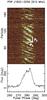 |
Fig. 1 Example sequence of about 200 successive pulses of PSR J1822−2256 observed using the GMRT at 610 MHz. The subpulses appear earlier with increasing pulse number and are arranged into so-called “drift bands”. There are two distinct drift modes visible: a fast mode seen in the first 60 pulses followed by a slow mode. The two successive drift bands are vertically separated by P3 periods and horizontally separated by P2 degrees in phase as indicated for the slow mode. The slow drift mode is followed by a null between pulse number 144 and 176. |
2. Source selection
We selected pulsars with an expected signal-to-noise ratio (S/N) of more than 3 that can be observed using the ORT at 326.5 MHz and at least seven antennas of a GMRT phased array at 610 MHz. The S/N was calculated with the radiometer equation, where the pulse width was adjusted to take into account the scatter broadening estimated using NE2001 model (Cordes & Lazio 2002). Additionally, the sky background was also taken into account using published all sky maps (Haslam et al. 1982) to estimate the system equivalent flux density. The sample was further refined by restricting the declination range within − 53° to 55°, which is the intersection of visible sky with both the ORT and the GMRT. After this selection, we checked the literature for any previously available single pulse studies of the remaining pulsars in the list. We selected those pulsars that have previously reported interesting single pulse behaviour, namely, prominent nulling or drifting and those that reported changes in the drift rates or multiple drift modes. Out of this list, we selected a subset of pulsars, where frequency dependent subpulse drift was reported in the past. We chose PSR B1237+25 as a control pulsar to test our analysis pipeline. Only pulsars with no previously reported simultaneous multi-frequency single pulse study were selected. We were able to observe a total 12 pulsars during the time allocated for the survey (Table 1).
3. Observations
All the observations were carried out using the ORT (Swarup et al. 1971) and the GMRT (Swarup et al. 1991). The GMRT was used in a phased array mode with two sub-arrays consisting of about nine 45 m antennas, one of which is at 610 MHz and the other at 1308 MHz bands, with a 33 MHz bandwidth. The phased array output for each of the two frequencies was recorded with 512 channels over the passband using the GMRT software baseband receiver with an effective sampling time of 1 ms along with a time stamp for the first recorded sample, which is derived from a GPS disciplined Rb frequency standard. The variations in the ionospheric and instrumental delays across the GMRT sub-arrays have a typical timescale of about 45 min at the observed frequencies. Hence, the observations were typically divided into two observing sessions, each of 45 min, interspersed with compensation for the instrumental delay drift to maintain phasing of the sub-array. The observations at the ORT were carried out using PONDER (Naidu et al. 2015). The observing band was centred at 326.5 MHz with a bandwidth of 16 MHz. The details of the observations are listed in Table 1.
4. Analysis
4.1. Pulse sequences
The data from both the observatories were converted into the standard format required for the SIGPROC1 analysis package and dedispersed using the programmes provided in the package. These were then folded to 1024 bins across the period using the ephemeris of these pulsars obtained with the TEMPO2 package to obtain a single pulse sequence (see Fig. 1). The pulse sequences at different frequencies were aligned as follows. First, the pulse sequence for the longest data file, typically consisting of 2000 pulses, was averaged for each frequency to obtain an integrated profile, which was used to form a noise-free template after centring the pulse for the pulsar at that frequency. Samples from the beginning of each file were removed so that the pulse was centred in a period using the template for the corresponding frequency. Then, time stamps for single pulses were corrected by these offsets. These were converted to a solar system barycentre via TEMPO22 (Hobbs et al. 2006; Edwards et al. 2006) taking into account the delay at lower frequencies due to dispersion in the interstellar medium. Then, the pulses corresponding to identical time stamps at the solar system barycentre across all frequencies were extracted from the data to get pulse sequences aligned across frequencies. An example of such simultaneous multi-frequency single pulse sequences is given in Fig. 3. Plots of these pulse sequences for the complete sample are available in Appendix A. The single pulse sequences were then visually examined to remove any single pulses with excessive radio frequency interference.
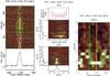 |
Fig. 2 Example showing the results of the analyses using the LRFS, 2DFS, and S2DFS techniques for PSR J1822−2206. Left: single pulse sequence of PSR J1822−2206 showing the drift bands with different drift rates and a null. Middle: LRFS and 2DFS plots of the single pulse sequence shown at left. The top plot is LRFS with the ordinate as P0/P3 and abscissa is the pulse phase. The top panel of LRFS is the integrated pulse profile along with the longitude-resolved modulation index (red line with the error bars). The bottom plot has the same ordinate as the top plot, but its abscissa is in units of P0/P2. The bottom panel in 2DFS shows the fluctuation frequency across a pulse integrated vertically between the indicated dashed lines around a feature. The left panels in the both LRFS and 2DFS plots are the spectra, integrated horizontally across the corresponding colour plot. Right: P3 S2DFS map made from the observation at 610 MHz using the GMRT. The vertical axis is given in P0/P3. The horizontal axis is given in blocks, where a block corresponds to average over N (typically 256) pulses. Periodic subpulse modulation is indicated by the “tracks” in this plot. The red, green, and yellow zones indicate the blocks corresponding to zones indicated with similar colour in the single pulse sequence shown in the leftmost plot. |
 |
Fig. 3 Example sequence of about 150 successive pulses of PSR B2016+28 observed simultaneously at three different frequencies (326.5 MHz with the ORT, and 610 and 1308 MHz with the GMRT). |
A suitable flux calibrator is observed for a short duration followed by a short observation of cold sky for all the observation sessions at GMRT and few sessions at the ORT. The averaged profile of the pulsar is calibrated with the appropriate scaling factor obtained from the ratio of averaged power on the flux calibrator to averaged power of the cold sky (see bottom plot of Fig. 1). For rest of the observations at the ORT, we used the average profile of the pulsar obtained by adding all single pulses; an on-pulse and off-pulse window, including the phase (where the pulse was present and absent, respectively) in which an equal number of bins were identified. A scaling factor was obtained by comparing the root mean square in the off-pulse window with the expected system equivalent flux density of the relevant telescope. The single pulse sequences were scaled with this factor and averaged to obtain a calibrated average profile. To estimate the nulling fraction, on-pulse and off-pulse energy sequences were formed by calculating the intensities in all samples in the on-pulse and off-pulse windows. These were used to obtain on-pulse and off-pulse energy distributions. Nulling fractions were obtained from these distributions following the method described in Gajjar et al. (2012).
The pulse sequences were further analysed using the techniques discussed in following subsections.
4.2. Fluctuation analysis
In bright pulsars, drifting subpulses, nulling, and mode changing can be detected just by visual inspection of the single pulse sequence. Backer (1970b,a) and Backer et al. (1975) were the first to use the Fourier analysis techniques to characterize P3. This often used technique is known as longitude-resolved fluctuation spectrum (LRFS). While LRFS is useful to estimate P3, it does not determine P2 and hence the drift rate. Edwards & Stappers (2002) presented a modified technique called the two-dimensional fluctuation spectrum (2DFS) to simultaneously estimate P2 and P3. Both these methods describe drifting in an averaged sense and are insensitive to its temporal behaviour, which is important for our investigation. Serylak et al. (2009) developed a technique called the sliding two-dimensional fluctuation spectrum (S2DFS), based on 2DFS, to provide information about the temporal changes that we are interested in. We used all three techniques and Fig. 2 shows an example of application of these techniques. As part of this work, we developed a single pulse analysis code to implement these techniques and this code was used in the analysis of our observations. These techniques are explained briefly in the following sections.
4.2.1. Longitude-resolved fluctuation spectrum
The pulse sequence was divided into adjacent blocks of N pulses (typically N ~ 256) and a discrete Fourier transform (DFT) was applied, at each pulse longitude bin in each block, to obtain LRFS for that block. The final spectrum is produced by averaging the LRFS of all blocks. Pulsars exhibiting periodically modulated subpulses have a region, the so-called feature, of enhanced spectral power that is visible as a bright region in the LRFS. The middle top plot in Fig. 2 shows the LRFS for the pulse sequence shown in the left plot of that figure. The frequency is given in cycles per period (cpp) and its inverse corresponds to the pattern periodicity, P3, expressed in pulsar periods P0. The position of the feature along the abscissa denotes the pulse longitude at which the modulation occurs. The subplot on top in the middle panel shows the integrated profile of PSR J1822−2206, normalized to the peak intensity, as a solid line. The red line with the error bars in this plot is the longitude-resolved modulation index (Edwards & Stappers 2002). The longitude-resolved modulation index is the measure of the amount by which the intensity varies from pulse to pulse for each pulse longitude.
4.2.2. Two-dimensional fluctuation spectrum
The LRFS can be used only to estimate P3. We use 2DFS to obtain both P2 and P3. This method is similar to the calculation of the LRFS, but the DFT is applied twice. First, the DFT of the pulse sequence along the constant pulse longitude is recorded. Then, the DFT across each row of the complex LRFS is obtained. In Fig. 2, the 2DFS for observations of PSR J1822−2256 at 610 MHz is plotted below the LRFS plot. The vertical axis of the resulting spectra are the same as in the LRFS, but the horizontal axis now corresponds to the horizontal separation of the drift bands. If the drifting subpulses have a preferred drift direction, then a feature is seen offset from the vertical axis (P0/P2 = 0). The 2DFS is vertically (between dashed lines) and horizontally integrated, resulting in the side and bottom panels. Estimates of P2 and P3, quoted in Tables 2 and 3, were calculated using the centroid of a rectangular region in the 2DFS containing the feature.
4.2.3. Sliding two-dimensional fluctuation spectrum
The LRFS and 2DFS are very effective for detecting and analysing subpulse modulation. Integrating multiple fluctuation spectra obtained from consecutive blocks of pulses increases the S/N of the resulting spectrum. However, this averaging does not reflect the temporal changes in drifting. To resolve the drift rate changes in the temporal domain, we used the S2DFS technique developed by Serylak et al. (2009). This method is an extension of the 2DFS. Here, 2DFS is computed for a block of a chosen number of pulses and collapsed over phase horizontally producing a longitude averaged fluctuation spectrum for the block (panel on left in 2DFS plot or LRFS plot in Fig. 2). The DFT window is then shifted by one pulse and the whole process is repeated, effectively sliding the window along the pulse sequence. This exercise of sliding the window and calculating the collapsed spectra results in N − M + 1 curves, where N is the number of pulses in the pulse sequence and M is the length of the DFT (block). These curves are arranged horizontally to form a map of collapsed fluctuation spectra called as S2DFS map. The right plot of Fig. 2 shows an example of the S2DFS map, where one can easily see the “drift tracks” (regions of enhanced intensity visible as a bright region). The changes in periodic modulation with time, clearly visible in the colour plot of this P3 S2DFS map, reflect changes in drifting. We used this analysis on pulse sequences, aligned across multiple frequencies, to study the simultaneity of changes in drifting across frequencies.
Modulation index and drift parameters for pulsars with independent multi-frequency observations.
The choice of length of the DFT window is crucial for the resolution and sensitivity of these maps. For shorter Fourier transforms or a smaller DFT window, the S2DFS maps would lack the spectral resolution in P0/P3 required to resolve the changes in the drift rates. Conversely, a longer Fourier transform or larger DFT window would reduce the sensitivity to any short-lasting events due to both the reduced S/N per spectral bin and a coarser temporal resolution. The duration of drift modes varies from pulsar to pulsar. Hence, the DFT length was selected by trial and error with block size ranging from 32 to 1024 pulses in logarithmic steps of 2. The optimum block size was selected by examining the corresponding pulse sequence plots and LRFS. In Fig. 2, we used a window with 32 pulses as the duration of the fast drift mode is about 42 periods. The change in P3 between the red, green, and yellow windows is indicated on the pulse sequence on the left plot in Fig. 2. During the transition from fast to slow drift the corresponding spectrum may be insensitive to both the modes.
Modulation index and drift parameters for pulsars with simultaneous multi-frequency observations.
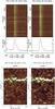 |
Fig. 4 Example sequences of about 600 successive pulses of PSR B1540−06 observed at two different frequencies is presented in the top plot. The corresponding S2DFS plots using a window size of 64 pulses are shown in the lower plots. |
The usefulness of S2DFS to investigate temporal subpulse drifting behaviour is apparent in Fig. 4. The single pulse sequences and corresponding S2DFS plots for PSR B1540−06 at two frequencies in simultaneous observations are shown in this figure. The two S2DFS plots show changes in P3 simultaneously at both the frequencies. Hence, this technique is very useful for our study concerning the broadband nature of the subpulse drifting for our sample of pulsars.
5. Results
The results of our analyses are presented in the Tables 2 and 3. The single pulse sequences, LRFS, 2DFS, and S2DFS plots for all pulsars along with the on-pulse energy sequences for four pulsars are available in Appendix A. We highlight salient features of individual pulsars in this section.
5.1. Non-simultaneous observations
PSR J0934−5249: this pulsar was observed at a single frequency (325 MHz) with the GMRT. Its single pulse sequence shows clear coherent drifting with some short nulls (Fig. A.1). The 2DFS (see Fig. A.2) plot also shows a clear feature, which confirms that this pulsar is a coherent drifter. The number of nulls were small for us to study any null induced drift rate changes in this pulsar. We are reporting estimates for drift and nulling parameters (Table 2) in this pulsar for the first time.
PSR J1822−2256: this pulsar was observed at a single frequency (610 MHz) with the GMRT. It shows regular drifting with changes in drift rates as is evident in Fig. 2. The 2DFS plot in this figure shows a clear feature. However, the drift rate changes seen in the single pulse sequence are not clearly visible in the 2DFS plot, which is probably due to the dominance of the slower drift mode in the selected pulse sequence. Here, S2DFS analysis is clearly very useful as it not only brings out two almost harmonically related drift modes, but also temporal timescales for these drift modes. Our results confirm the two drift rates seen by WES06 at 21-cm. Later studies by WES07 and Basu et al. (2016) detected only one drift rate (P3 ~ 17P0). While our observations were at 610 MHz only, we detect both modes in our observations. The previous non-detection at lower frequency is probably due to short observations, where only one mode might have been present. Hence, our result along with the presence of multiple drift modes implies a broadband drift behaviour. The single pulse sequence shows regular nulls leading, which confirms reported pulse nulling by Burke-Spolaor et al. (2012). We report the nulling fraction, i.e. 10 ± 2%, for this pulsar for the first time. The single pulse properties of this pulsar are very similar to PSR B0031−07 (Vivekanand & Joshi 1997) owing to presence of nulling and harmonically related drift modes.
PSR J1901−0906: this pulsar was observed at two different frequencies (325 MHz and 610 MHz) independently using the GMRT. The integrated profile has two widely separated components (see Fig. A.25). The drifting is clearly visible in the pulse sequence as is pulse nulling. WES06 first reported drifting in this pulsar at 21 cm and concluded that it shows drifting with two distinct values of P3 (3 and 7 P0). They detected the former mode only in the trailing component, while the latter was seen in both components. Also, WES07 adetected drifting at 92 cm with two different P3 (3 and 5 P0), where the latter value is different from that seen at 21 cm. These authors concluded that this pulsar shows differences in subpulse drift not only in its two components, but also between the two frequencies. Our longer and higher sensitivity observations suggest that the pulsar exhibits three distinct drift modes in both of the components (see Table 2) at both 325 and 610 MHz. The fast drift mode is more prominent in the trailing component, while the slow modes are more prominent in the leading component (see Fig. A.26). This is probably one of the reasons for difference in drift properties of the two components seen by WES06. The different measured P3 values in the two components confirms that this pulsar is a drift mode changer. Interestingly, the two components do not exhibit subpulse drift with identical P3 as can be seen in S2DFS plots of the two components (Fig. A.27). The frequency dependent and component dependent drift reported by WES06 and WES07 most likely arises because of this complex subpulse behaviour seen in our observations. Our observations suggest a broadband drifting behaviour in this pulsar. J1901−0906 also shows several prominent nulls. We report the nulling fraction for this pulsar for the first time (Table 2). This is a unique and interesting pulsar that exhibits not only multiple distinct drift modes, similar to PSR B0031−07, but also exhibits different drift modes in two widely separated components. This result should motivate consideration of future long simultaneous multi-frequency observations of this pulsar.
5.2. Simultaneous observations
PSR B1237+ 25: this pulsar has a multi-component profile and was observed simultaneously at 326.5 MHz and 610 MHz with the ORT and GMRT, respectively. Single pulse sequences at both frequencies are shown in Fig. A.4, which indicates a correlated single pulse behaviour including nulls at both frequencies. On-pulse energy sequences, shown in Fig. A.10, suggest that the pulsar nulls simultaneously at both frequencies. Nulling fraction estimated from our observations (Table 3) are consistent with that reported previously (Ritchings 1976). WES06 reported a detection of fast mode (P3 ~ 2.8P0) in all components at 21 cm and in three components at 92 cm. We detected a similar mode at both 326.5 and 610 MHz in the leading and trailing components (Fig. A.5). We also detected a slow mode (P3 ~ 28 ± 8 P0) in the central component at 326.5 MHz consistent with that reported by Maan & Deshpande (2014; see Fig. A.6). Simultaneous 610 MHz data show the same feature but with lower intensity. Thus, our observations are consistent with previous studies of drifting in this pulsar. In addition, S2DFS analysis shows that the temporal behaviour of the drifting subpulses is similar at both frequencies (see Fig. A.7).
PSR B1508+55: observations were carried out at three frequencies. The single pulse S/N was low at 326.5 and 1308 MHz, whereas observations at 610 MHz show strong single pulses (Fig. A.11). The 2DFS plots show a broad low frequency feature. Pulsar shows clear nulls in single pulse sequences, which appear to be correlated across 326.5 and 610 MHz (Fig. A.13). We report pulse nulling for the first time in this pulsar and the nulling fraction is estimated to be 7 ± 2%.
PSR B1540−06: the simultaneous observations of this pulsar were carried out at 610 and 326.5 MHz, respectively. There is strong feature at 3.0 ± 0.2 P0 in the 2DFS plot at both frequencies (Fig. A.15). Our measurement is consistent with previous studies (WES07). The S2DFS plots show that P3 varies a bit, but the changes in drift are simultaneous (Fig. A.16). There appear to be some nulls, but the S/N at 326.5 MHz was not sufficient to detect such nulls. Nulls are more discernible at 610 MHz and we estimate the nulling fraction to be about 6 percent (Fig. A.14).
PSR B1718−32: observations of this pulsar were carried out at three different frequencies (326.5, 610 and 1308 MHz). The single pulse S/N was low at 326.5 MHz and 1308 MHz, but strong single pulses were seen at 610 MHz (Fig. A.17). The 2DFS plot (Fig. A.18) shows a bright feature at about 22 ± 3 P0. Visual examination of single pulse sequence reveals that this feature is due to amplitude modulation of the leading component and does not appear to be subpulse drifting. We report this modulation feature for the first time. No significant nulling is detected in this pulsar.
PSR B1844−04: the single pulse S/N for this pulsar at the ORT was low and only single pulses from the GMRT observations were useful for further analysis (Fig. A.20). The LRFS shows a broad low frequency feature at 11 ± 2 P0 (see Fig. A.21). WES06 detected this feature at the 21 cm waveband but not at the 92 cm waveband. The profile at 326.5 MHz is scatter-broadened, which masks subpulse drifting and this could be the reason for non-detection of a drift feature in our observations as well as past observations.
PSR B1845−19: no significant drifting is observed at any of the three frequencies. The pulsar nulls frequently and nulls are simultaneous at 326.5 and 610 MHz (Figs. A.23 and A.24). We report pulse nulling for the first time in this pulsar with nulling fraction estimated to be 27 ± 6%.
PSR B2016+28: this pulsar shows prominent drift bands at all three frequencies. The drift pattern is variable, but correlated across the three frequencies (Fig. 3). This is in contrast with results reported by Oster et al. (1977) suggesting a frequency dependent subpulse drift. Indeed, a feature detected in 2DFS plot at 1308 MHz is not apparent at 326.5 MHz (Fig. A.29), which is consistent with a similar result reported by WES06 and WES07. However, a weak feature is present at 610 MHz (and possibly at 326.5 MHz) in the 2DFS plot for the leading component of the integrated profile for this pulsar (Fig. A.30). Moreover, there are few sections of data, where this component is detected at all three frequencies as is evident in S2DFS plot for one such section (Fig. A.32). Lastly, the temporal changes in the S2DFS plot (Fig. A.31) indicate that the drift pattern changes simultaneously at all frequencies. As the drift rate varies from band to band resulting in the broad features in the LRFS, analyses of short and/or non-simultaneous observations can mimic a frequency dependence, which is not borne out by our longer simultaneous observations. Thus, we conclude that drifting is independent of frequency of observations. The pulsar does not show any significant nulling.
PSR B2043−04: the single pulse S/N of this pulsar at 1308 MHz was low during our observations (Fig. A.33), but 326.5 and 610 MHz data show a strong feature at 2.7 ± 0.1 P0 in our 2DFS analysis (Fig. A.34). Although single pulses are not visible at 1308 MHz, this feature is also present in 2DFS at 1308 MHz. There is also a very weak feature at 3.7 P0, seen in 2DFS plots (see Figs. A.34 and A.35). Sometimes the P3 varies with these changes occurring simultaneously at 326.5 and 610 MHz (Fig. A.36). No significant nulls are observed in this pulsar.
PSR B2045−16: this pulsar has a multiple component profile. A variety of single pulse behaviour along with prominent nulls are seen in the single pulse plots (Fig. A.37). A broad feature with P3 values between 2 and 3 P0 were reported in the outermost components in some previous studies (Oster et al. 1977; Nowakowski et al. 1982), whereas drifting with P3 = 3.2P0 was only reported in the trailing component at 21 cm waveband (WES06). In contrast, WES07 reported drifting in three components at the 92 cm waveband with P3 varying between 2.7 to 3 P0 as well as a low frequency feature with P3 = 32P0. Our 2DFS analysis shows a strong feature at 3.2 P0 in the leading and trailing components (see Fig. A.38). These features are also evident in S2DFS plots for 326.5 and 610 MHz (Fig. A.39). These plots indicate that the fluctuation frequency varies between 3.57 P0 to 2.5 P0 in all components and the changes in P3 occur simultaneously across all frequencies, including 1308 MHz, where WES06 reported drifting only in the trailing component. Thus, drifting behaviour appears to be broadband in this pulsar and any differences reported in the past can be attributed to drift modes in this pulsar and non-simultaneity of observations. The pulsar exhibits nulling and its nulling fraction is tabulated in Table 3. The nulls seem to be broadband (Fig. A.40) and the nulling fraction is consistent across all frequencies.
6. Discussion
The results from our simultaneous multi-frequency single pulse observations of nine pulsars with subpulse drifting or nulling are presented in this paper. We also report on single frequency observations for three pulsars. We report subpulse drifting in PSR J0934−5249 for the first time. We also report pulse nulling measurements in PSRs J0934−5249, B1508+55, J1822−2256, B1845−19, and J1901−0906 for the first time. Our measurements of subpulse drifting and pulse nulling for the rest of the pulsars are consistent with previously reported values.
Most of the pulsars in our sample were observed at two or more frequencies simultaneously. We made an attempt to understand the fluctuation properties of these pulsars by examining single pulse sequences, LRFS, 2DFS, and S2DFS analyses. To examine the temporal changes in drift pattern, we used S2DFS method. The simultaneous temporal changes are investigated across the frequencies with both visual and S2DFS analyses to check for any frequency dependent behaviour.
Our results confirm and further strengthen the conclusions drawn by WES06 and WES07, in which these authors state that subpulse drifting is broadband in general. Our sample consisted of pulsars with reported differences in P3 at different frequencies by these authors and by other past studies. For example, non-simultaneous short observations by WES06 and WES07 suggested different P3 values at 21 cm and 92 cm for PSRs J1822−2256, J1901−0906, B1844−04, B2016+28, and B2045−16. Similarly, drifting was seen in only one component of the integrated profile in PSRs J1901−0906, B2016+28, and B2045−16 at one or both frequencies in their study. Frequency dependent subpulse drifting was suggested in at least two past studies (Oster et al. 1977; WES06; WES07). As mentioned before, this could be due to (a) the dependence of subpulse drifting mechanism on emission height and, therefore, observing frequency by virtue of radius-to-frequency mapping; (b) the geometric origin manifested in profile evolution; or (c) the presence of drift modes or variation in drift rate, which leads to an apparent difference due to short duration observations and the non-simultaneous nature of these studies. In our work, we examined the drift behaviour with longer (typically 90 min) simultaneous multi-frequency observations to distinguish between these three possibilities. Contrary to previous belief, we find no evidence for a frequency dependent drift pattern in PSR B2016+28 implied by non-simultaneous observations by Oster et al. (1977). In PSR B1237+25, J1822−2256, J1901−0906, and B2045−16, our longer and more sensitive observations reveal multiple drift rates with distinct P3, which is consistent with the values reported previously using observations where probably only a given mode was present. Additionally, our S2DFS analysis of pulse sequences aligned across frequencies show changes in P3 occurring at the same time across frequencies for these pulsars. This is also true for other pulsars, except PSR B1844−04, where scatter-broadening masks drifting at 326.5 MHz. Thus, we conclude that subpulse drift is broadband even in these pulsars and multiple drift modes can give the appearance of a frequency dependence if, first, the observation duration is smaller than the timescales required to sample all modes or, second, a given drift mode is rare. The implied broadband nature also suggests that geometry of pulsar emission including variations with emission heights are unlikely to affect the drift periodicities.
Some of the pulsars in our sample also exhibit pulse nulling. The single pulse sequences were visually examined and nulling seemed to be simultaneous across all the observed frequencies. The nulling fractions at different frequencies are consistent. Thus, pulse nulling appears to be broadband in these pulsars. A recent multi-frequency study of three pulsars with long observations has reported broadband nulling in those pulsars (Gajjar et al. 2014a). We added four more pulsars to this list, thereby increasing the sample of such pulsars by more than 100 percent.
Establishing a broadband nature of these phenomena is important for the following reasons. Profile evolution with frequency implies that the frequency of choice for studies of drifting can be different for different pulsars. Once, it is broadly established that drifting (and nulling behaviour) is concurrent across the observing frequency, an appropriate frequency can be chosen for more sensitive observations. Moreover, deeper studies can then be made to characterize changes in drift behaviour, which may be related to profile mode changes. Recently, it has been shown that off state in intermittent pulsars and pulsars with profile mode changes are accompanied by changes in spin-down rate (Lyne et al. 2010). Long follow-up observations with appropriately chosen frequency will therefore be very useful in understanding the switching behaviour of the magnetosphere, which has been invoked to explain the spin-down changes mentioned above (Timokhin 2010). With multi-beam capability in upcoming large collecting area telescopes, such as Square Kilometer Array (SKA), such long-term observations are possible and our study allows careful choice of frequency band in SKA for this purpose.
The lack of corotation of localized “sparks” in the polar gap, defined by the open field lines, was invoked by Ruderman & Sutherland (1975) to explain the subpulse drift. In this model, the relativistic outflow of electron-positron from these “sparks” produces the subpulse associated radio emission higher up in the magnetosphere. The local plasma frequency and magnetic field at a given height determine the frequency of radio emission emitted at that height, which is also referred to as “radius-to-frequency mapping” (Cordes 1978). As the “sparks” lag behind the rotation of the star, the associated radio emission also progressively changes its phase within the period, which is seen as subpulse drift with subpulses associated with each “spark”. In this model, the drift is likely to be similar at different frequencies as it is determined solely by the motion of “sparks”, which is governed by the gap potential and magnetic field in the polar gap. Hence, subpulse drift is broadband in this model in contrast with models invoking dependence on viewing geometry.
Finally, in Ruderman & Sutherland (1975) model, the drift rate of subpulses provides a fundamental probe of the polar cap physics and the changes in the state of the magnetosphere. If profile mode changes (including nulls) are related to drifting, as established in PSR B0031−07 (Vivekanand & Joshi 1997) and B2319+60 (Wright & Fowler 1981), a study of these phenomena over multiple frequencies can provide useful constraints on magnetospheric physics. Our study points out three more candidates for such studies. These are PSR J1822−2256, J1901−0906, and B2045−16, where longer observations, similar to ours are motivated. Upcoming telescopes such as SKA can enhance this sample substantially apart from providing higher sensitivity pulse sequences.
7. Conclusions
The observations presented in this paper provide further confirmation that the subpulse drift and pulse nullingare predominantly broadband consistent with previous studies (Gajjar et al. 2014a; Rankin 1986, WES07). While this is expected from models such as Ruderman & Sutherland (1975), we have dealt with some of previously reported exceptions in this paper and find that any frequency dependent behaviour can be attributed to multiple drift modes. Our results thus suggest that the origin of drifting and pulse nulling is closely tied to the physics of polar gap.
Acknowledgments
We thank the staff of the Ooty Radio Telescope and the Giant Meterwave Radio Telescope for making these observations possible. Both these telescopes are operated by National Centre for Radio Astrophysics (TIFR). This work made use of PONDER backend, built with TIFR XII plan grants 12P0714 and 12P0716. We like to thank the anomynous referee for useful comments and suggestions. A.N. would like to thank Dave Green and Yogesh Maan for providing the colour scheme used for the plots. B.C.J., P.K.M., and M.A.K. acknowledge support for this work from DST-SERB grant EMR/2015/000515.
References
- Backer, D. C. 1970a, Nature, 228, 752 [NASA ADS] [CrossRef] [Google Scholar]
- Backer, D. C. 1970b, Nature, 227, 692 [NASA ADS] [CrossRef] [Google Scholar]
- Backer, D. C., Rankin, J. M., & Campbell, D. B. 1975, ApJ, 197, 481 [NASA ADS] [CrossRef] [Google Scholar]
- Bartel, N. 1981, A&A, 97, 384 [NASA ADS] [Google Scholar]
- Bartel, N., & Sieber, W. 1978, A&A, 70, 307 [NASA ADS] [Google Scholar]
- Basu, R., Mitra, D., Melikidze, G. I., et al. 2016, ApJ, 833, 29 [NASA ADS] [CrossRef] [Google Scholar]
- Bhat, N. D. R., Gupta, Y., Kramer, M., et al. 2007, A&A, 462, 257 [NASA ADS] [CrossRef] [EDP Sciences] [Google Scholar]
- Biggs, J. D. 1992, ApJ, 394, 574 [NASA ADS] [CrossRef] [Google Scholar]
- Burke-Spolaor, S., Johnston, S., Bailes, M., et al. 2012, MNRAS, 423, 1351 [NASA ADS] [CrossRef] [Google Scholar]
- Cordes, J. M. 1978, ApJ, 222, 1006 [NASA ADS] [CrossRef] [PubMed] [Google Scholar]
- Cordes, J. M., & Lazio, T. J. W. 2002, ArXiv e-prints [arXiv:astro-ph/0207156] [Google Scholar]
- Davies, J. G., Lyne, A. G., Smith, F. G., et al. 1984, MNRAS, 211, 57 [NASA ADS] [CrossRef] [Google Scholar]
- Edwards, R. T., & Stappers, B. W. 2002, A&A, 393, 733 [NASA ADS] [CrossRef] [EDP Sciences] [Google Scholar]
- Edwards, R. T., Hobbs, G. B., & Manchester, R. N. 2006, MNRAS, 372, 1549 [NASA ADS] [CrossRef] [Google Scholar]
- Gajjar, V., Joshi, B. C., & Kramer, M. 2012, MNRAS, 424, 1197 [NASA ADS] [CrossRef] [Google Scholar]
- Gajjar, V., Joshi, B. C., Kramer, M., Karuppusamy, R., & Smits, R. 2014a, ApJ, 797, 18 [NASA ADS] [CrossRef] [Google Scholar]
- Gajjar, V., Joshi, B. C., & Wright, G. 2014b, MNRAS, 439, 221 [NASA ADS] [CrossRef] [Google Scholar]
- Haslam, C. G. T., Salter, C. J., Stoffel, H., & Wilson, W. E. 1982, A&AS, 47, 1 [NASA ADS] [Google Scholar]
- Hobbs, G. B., Edwards, R. T., & Manchester, R. N. 2006, MNRAS, 369, 655 [NASA ADS] [CrossRef] [Google Scholar]
- Huguenin, G. R., Taylor, J. H., & Troland, T. H. 1970, ApJ, 162, 727 [NASA ADS] [CrossRef] [Google Scholar]
- Joshi, B. C., & Vivekanand, M. 2000, MNRAS, 316, 716 [NASA ADS] [CrossRef] [Google Scholar]
- Kramer, M., Lyne, A. G., O’Brien, J. T., Jordan, C. A., & Lorimer, D. R. 2006, Science, 312, 549 [NASA ADS] [CrossRef] [PubMed] [Google Scholar]
- Lyne, A. G. 1971, MNRAS, 153, 27 [NASA ADS] [CrossRef] [Google Scholar]
- Lyne, A. G., & Ashworth, M. 1983, MNRAS, 204, 519 [NASA ADS] [Google Scholar]
- Lyne, A., Hobbs, G., Kramer, M., Stairs, I., & Stappers, B. 2010, Science, 329, 408 [NASA ADS] [CrossRef] [PubMed] [Google Scholar]
- Maan, Y., & Deshpande, A. A. 2014, ApJ, 792, 130 [NASA ADS] [CrossRef] [Google Scholar]
- McLaughlin, M. A., Lyne, A. G., Lorimer, D. R., et al. 2006, Nature, 439, 817 [NASA ADS] [CrossRef] [PubMed] [Google Scholar]
- Naidu, A., Joshi, B. C., Manoharan, P. K., & Krishnakumar, M. A. 2015, Exp. Astron., 39, 319 [NASA ADS] [CrossRef] [Google Scholar]
- Nowakowski, L., Usowicz, J., Kepa, A., & Wolszczan, A. 1982, A&A, 116, 158 [NASA ADS] [Google Scholar]
- Oster, L., Hilton, D. A., & Sieber, W. 1977, A&A, 57, 1 [NASA ADS] [Google Scholar]
- Rankin, J. M. 1986, ApJ, 301, 901 [NASA ADS] [CrossRef] [Google Scholar]
- Ritchings, R. T. 1976, MNRAS, 176, 249 [NASA ADS] [Google Scholar]
- Ruderman, M. A., & Sutherland, P. G. 1975, ApJ, 196, 51 [NASA ADS] [CrossRef] [EDP Sciences] [Google Scholar]
- Serylak, M., Stappers, B. W., & Weltevrede, P. 2009, A&A, 506, 865 [NASA ADS] [CrossRef] [EDP Sciences] [Google Scholar]
- Sieber, W., & Oster, L. 1975, A&A, 38, 325 [NASA ADS] [Google Scholar]
- Smits, J. M., Mitra, D., Stappers, B. W., et al. 2007, A&A, 465, 575 [NASA ADS] [CrossRef] [EDP Sciences] [Google Scholar]
- Sutton, J. M., Staelin, D. H., Price, R. M., & Weimer, R. 1970, ApJ, 159 [Google Scholar]
- Swarup, G., Sarma, N. V. G., Joshi, M. N., et al. 1971, Nat. Phys. Sci., 230, 185 [NASA ADS] [CrossRef] [Google Scholar]
- Swarup, G., Ananthakrishnan, S., Kapahi, V. K., et al. 1991, Current Science, 60, 95 [Google Scholar]
- Taylor, J. H., Manchester, R. N., & Huguenin, G. R. 1975, ApJ, 195, 513 [NASA ADS] [CrossRef] [Google Scholar]
- Timokhin, A. N. 2010, MNRAS, 408, L41 [NASA ADS] [CrossRef] [Google Scholar]
- Vivekanand, M., & Joshi, B. C. 1997, ApJ, 477, 431 [NASA ADS] [CrossRef] [Google Scholar]
- Wang, N., Manchester, R. N., & Johnston, S. 2007, MNRAS, 377, 1383 [NASA ADS] [CrossRef] [Google Scholar]
- Weltevrede, P., Edwards, R. T., & Stappers, B. W. 2006, A&A, 445, 243 [NASA ADS] [CrossRef] [EDP Sciences] [Google Scholar]
- Weltevrede, P., Stappers, B. W., & Edwards, R. T. 2007, A&A, 469, 607 [NASA ADS] [CrossRef] [EDP Sciences] [Google Scholar]
- Wright, G. A. E., & Fowler, L. A. 1981, A&A, 101, 356 [NASA ADS] [Google Scholar]
Appendix A: Analysis plots
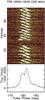 |
Fig. A.1 Single pulse sequence in PSR J0934−5249 zoomed to show a null. |
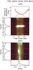 |
Fig. A.2 LRFS and 2DFS plots for PSR J0934−5249. A bright feature can be seen in the 2DFS plot classifying this pulsar as coherent drifter. |
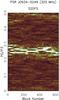 |
Fig. A.3 S2DFS of leading component of PSR J0934−5249. |
All the relevant plots from our analyses are given in this Appendix. Plots are arranged according to the pulsar name. A brief description of techniques and the plots is given below.
-
1.
Single pulse sequence: these plots are used for visualexamination of the single pulse sequences for drifting and nullingbehaviour. The colour plot is the stack of single pulses; the bottompanel is the integrated profile, where abscissa is the pulse phase indegrees, and the ordinate is the pulse flux density in milliJansky.
-
Longitude-resolved fluctuation spectra (LRFS): this plot is used to estimate pattern separation (P3). The colour plot is the LRFS with the ordinate as P0/P3 (P0 is the period of the pulsar) and abscissa is the pulse phase. The top panel of LRFS is the integrated pulse profile along with the longitude-resolved modulation index (red line with the error bars). The plot on left is the longitude averaged fluctuation spectra.
-
3.
Two-dimentional fluctuation spectra (2DFS): the subpulse separation (P2) is estimated using the 2DFS. The colour plot is the 2DFS with the ordinate as P0/P3 and abscissa is the in units of P0/P2. The bottom panel in 2DFS shows the fluctuation frequency across a pulse integrated vertically between the indicated dashed lines around a feature.
-
4.
Sliding two-dimensional fluctuation spectra (S2DFS): this technique is used to estimate the temporal variation of the P3. This plot is obtained by stacking the longitudinal averaged 2DFS spectra for pulses in the short imaginary window sliding along the pulse sequence. The ordinate of the colour plot is P0/P3 and abscissa is the corresponding block number.
-
5.
On-pulse sequence: these plots can be used to visualize the pulse energy variation across the frequencies. The ordinate is the significance of the on-pulse energy in units of standard deviation of the off-pulse energy and the abscissa is the pulse number. The black line in all these plots in the off-pulse energy.
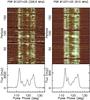 |
Fig. A.4 Single pulse sequences in PSR B1237+25 zoomed to show a null. |
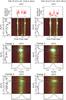 |
Fig. A.5 LRFS and 2DFS plots for PSR B1237+25. A clear drift feature, in both the trailing and leading components, is seen. There is a weak feature representing the slow drift mode that is difficult to distinguish in this plot. This is more easily seen in Fig. A.6. |
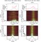 |
Fig. A.6 LRFS and 2DFS plots for the second component of PSR B1237+25. A low frequency drift feature can be seen in the LRFS at 326.5 MHz. A weak feature is also seen in the LRFS at 610 MHz. |
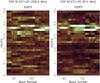 |
Fig. A.7 S2DFS of the leading component of PSR B1237+25. |
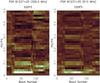 |
Fig. A.8 S2DFS of central component of PSR B1237+25. |
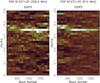 |
Fig. A.9 S2DFS of the trailing component of PSR B1237+25. |
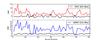 |
Fig. A.10 On-pulse energy sequence of PSR B1237+25. |
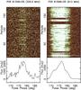 |
Fig. A.11 Single pulse sequence for PSR B1508−55. |
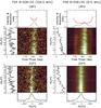 |
Fig. A.12 LRFS and 2DFS plots for PSR B1508+55. A broad low frequency feature in both the frequencies is seen. |
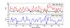 |
Fig. A.13 On-pulse energy sequence of PSR B1508−06. |
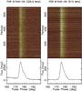 |
Fig. A.14 Single pulse sequence for PSR B1540−06. |
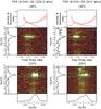 |
Fig. A.15 LRFS and 2DFS plots for B1540−06. A single bright feature at both the frequencies is seen. |
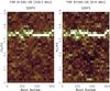 |
Fig. A.16 S2DFS of PSR B1540−06. |
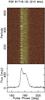 |
Fig. A.17 Single pulse sequence for PSR B1718−32. The single pulse S/N is low at 326.5 MHz and 1308 MHz observations. |
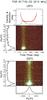 |
Fig. A.18 LRFS and 2DFS plots for PSR B1718−32. Strong drift feature is seen only at 610 MHz. Non-detection at other frequencies is probably due to the low S/N. |
 |
Fig. A.19 S2DFS of PSR B1718−32. |
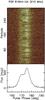 |
Fig. A.20 Single pulse sequences for PSR B1844−04. The single pulse S/N is low for 326.5 MHz observation. |
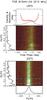 |
Fig. A.21 LRFS and 2DFS plots for PSR B1844−04. The plots show a broad feature at 610 MHz. |
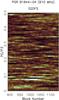 |
Fig. A.22 S2DFS of PSR B1844−04. |
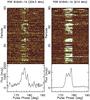 |
Fig. A.23 Single pulse sequences for PSR B1845−19. |
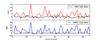 |
Fig. A.24 On-pulse energy sequence of PSR B1845+55. |
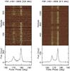 |
Fig. A.25 Single pulse sequences of independent observations at 325 MHz and 610 MHz using the GMRT for PSR J1901−0906. |
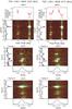 |
Fig. A.26 LRFS and 2DFS plots for PSR J1901−0906. Three three clear drift features are seen in both the components. Fast mode is more prominent in the trailing component. |
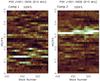 |
Fig. A.27 S2DFS for the two components of PSR J1901−0906 observed at 610 MHz. The plot on left is the S2DFS for the leading component and the plot on the right is for the trailing component. |
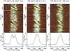 |
Fig. A.28 Single pulse sequences for PSR B2016+28. |
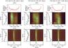 |
Fig. A.29 LRFS and 2DFS plots for PSR B2016+28. The 1308 MHz shows a clear low frequency feature in the leading component in the LRFS plot, which is also present as a weak feature at other frequencies. |
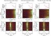 |
Fig. A.30 LRFS and 2DFS plots for leading component for PSR B2016+28. The low frequency feature is clearly seen at 1308 MHz, but is weaker at 326.5 and 610 MHz. |
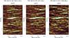 |
Fig. A.31 S2DFS of PSR B2016+28. |
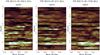 |
Fig. A.32 S2DFS of leading component of PSR B2016+28. |
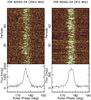 |
Fig. A.33 Single pulse sequence for PSR B2043−04. The single pulse S/N is low at 1308 MHz observations. |
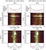 |
Fig. A.34 LRFS and 2DFS plots for PSR B2043−04. Bright narrow features can be seen at 326.5 MHz and 610 MHz. The S/N at 1308 MHz was low, but a very weak detection can be seen in LRFS at 1308 MHz. In addition, there is a very weak feature at about 0.3 cpp at both 610 and 326.5 MHz. |
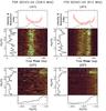 |
Fig. A.35 LRFS and 2DFS plots zoomed around 0.3 cpp for PSR B2043−04. A common feature can be seen at both 326.5 and 610.0 MHz. |
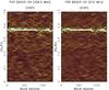 |
Fig. A.36 S2DFS of PSR B2043−04. |
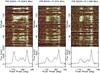 |
Fig. A.37 Single pulse sequences for PSR B2045−16 showing the simultaneous nulla and correlated subpulse behaviour. |
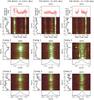 |
Fig. A.38 LRFS and 2DFS plots for PSR B2045−16. |
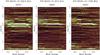 |
Fig. A.39 S2DFS of PSR B2045−16. |
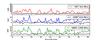 |
Fig. A.40 On-pulse energy sequence of PSR B2045−16. |
All Tables
Modulation index and drift parameters for pulsars with independent multi-frequency observations.
Modulation index and drift parameters for pulsars with simultaneous multi-frequency observations.
All Figures
|
Fig. 1 Example sequence of about 200 successive pulses of PSR J1822−2256 observed using the GMRT at 610 MHz. The subpulses appear earlier with increasing pulse number and are arranged into so-called “drift bands”. There are two distinct drift modes visible: a fast mode seen in the first 60 pulses followed by a slow mode. The two successive drift bands are vertically separated by P3 periods and horizontally separated by P2 degrees in phase as indicated for the slow mode. The slow drift mode is followed by a null between pulse number 144 and 176. |
| In the text | |
|
Fig. 2 Example showing the results of the analyses using the LRFS, 2DFS, and S2DFS techniques for PSR J1822−2206. Left: single pulse sequence of PSR J1822−2206 showing the drift bands with different drift rates and a null. Middle: LRFS and 2DFS plots of the single pulse sequence shown at left. The top plot is LRFS with the ordinate as P0/P3 and abscissa is the pulse phase. The top panel of LRFS is the integrated pulse profile along with the longitude-resolved modulation index (red line with the error bars). The bottom plot has the same ordinate as the top plot, but its abscissa is in units of P0/P2. The bottom panel in 2DFS shows the fluctuation frequency across a pulse integrated vertically between the indicated dashed lines around a feature. The left panels in the both LRFS and 2DFS plots are the spectra, integrated horizontally across the corresponding colour plot. Right: P3 S2DFS map made from the observation at 610 MHz using the GMRT. The vertical axis is given in P0/P3. The horizontal axis is given in blocks, where a block corresponds to average over N (typically 256) pulses. Periodic subpulse modulation is indicated by the “tracks” in this plot. The red, green, and yellow zones indicate the blocks corresponding to zones indicated with similar colour in the single pulse sequence shown in the leftmost plot. |
| In the text | |
|
Fig. 3 Example sequence of about 150 successive pulses of PSR B2016+28 observed simultaneously at three different frequencies (326.5 MHz with the ORT, and 610 and 1308 MHz with the GMRT). |
| In the text | |
|
Fig. 4 Example sequences of about 600 successive pulses of PSR B1540−06 observed at two different frequencies is presented in the top plot. The corresponding S2DFS plots using a window size of 64 pulses are shown in the lower plots. |
| In the text | |
|
Fig. A.1 Single pulse sequence in PSR J0934−5249 zoomed to show a null. |
| In the text | |
|
Fig. A.2 LRFS and 2DFS plots for PSR J0934−5249. A bright feature can be seen in the 2DFS plot classifying this pulsar as coherent drifter. |
| In the text | |
|
Fig. A.3 S2DFS of leading component of PSR J0934−5249. |
| In the text | |
|
Fig. A.4 Single pulse sequences in PSR B1237+25 zoomed to show a null. |
| In the text | |
|
Fig. A.5 LRFS and 2DFS plots for PSR B1237+25. A clear drift feature, in both the trailing and leading components, is seen. There is a weak feature representing the slow drift mode that is difficult to distinguish in this plot. This is more easily seen in Fig. A.6. |
| In the text | |
|
Fig. A.6 LRFS and 2DFS plots for the second component of PSR B1237+25. A low frequency drift feature can be seen in the LRFS at 326.5 MHz. A weak feature is also seen in the LRFS at 610 MHz. |
| In the text | |
|
Fig. A.7 S2DFS of the leading component of PSR B1237+25. |
| In the text | |
|
Fig. A.8 S2DFS of central component of PSR B1237+25. |
| In the text | |
|
Fig. A.9 S2DFS of the trailing component of PSR B1237+25. |
| In the text | |
|
Fig. A.10 On-pulse energy sequence of PSR B1237+25. |
| In the text | |
|
Fig. A.11 Single pulse sequence for PSR B1508−55. |
| In the text | |
|
Fig. A.12 LRFS and 2DFS plots for PSR B1508+55. A broad low frequency feature in both the frequencies is seen. |
| In the text | |
|
Fig. A.13 On-pulse energy sequence of PSR B1508−06. |
| In the text | |
|
Fig. A.14 Single pulse sequence for PSR B1540−06. |
| In the text | |
|
Fig. A.15 LRFS and 2DFS plots for B1540−06. A single bright feature at both the frequencies is seen. |
| In the text | |
|
Fig. A.16 S2DFS of PSR B1540−06. |
| In the text | |
|
Fig. A.17 Single pulse sequence for PSR B1718−32. The single pulse S/N is low at 326.5 MHz and 1308 MHz observations. |
| In the text | |
|
Fig. A.18 LRFS and 2DFS plots for PSR B1718−32. Strong drift feature is seen only at 610 MHz. Non-detection at other frequencies is probably due to the low S/N. |
| In the text | |
|
Fig. A.19 S2DFS of PSR B1718−32. |
| In the text | |
|
Fig. A.20 Single pulse sequences for PSR B1844−04. The single pulse S/N is low for 326.5 MHz observation. |
| In the text | |
|
Fig. A.21 LRFS and 2DFS plots for PSR B1844−04. The plots show a broad feature at 610 MHz. |
| In the text | |
|
Fig. A.22 S2DFS of PSR B1844−04. |
| In the text | |
|
Fig. A.23 Single pulse sequences for PSR B1845−19. |
| In the text | |
|
Fig. A.24 On-pulse energy sequence of PSR B1845+55. |
| In the text | |
|
Fig. A.25 Single pulse sequences of independent observations at 325 MHz and 610 MHz using the GMRT for PSR J1901−0906. |
| In the text | |
|
Fig. A.26 LRFS and 2DFS plots for PSR J1901−0906. Three three clear drift features are seen in both the components. Fast mode is more prominent in the trailing component. |
| In the text | |
|
Fig. A.27 S2DFS for the two components of PSR J1901−0906 observed at 610 MHz. The plot on left is the S2DFS for the leading component and the plot on the right is for the trailing component. |
| In the text | |
|
Fig. A.28 Single pulse sequences for PSR B2016+28. |
| In the text | |
|
Fig. A.29 LRFS and 2DFS plots for PSR B2016+28. The 1308 MHz shows a clear low frequency feature in the leading component in the LRFS plot, which is also present as a weak feature at other frequencies. |
| In the text | |
|
Fig. A.30 LRFS and 2DFS plots for leading component for PSR B2016+28. The low frequency feature is clearly seen at 1308 MHz, but is weaker at 326.5 and 610 MHz. |
| In the text | |
|
Fig. A.31 S2DFS of PSR B2016+28. |
| In the text | |
|
Fig. A.32 S2DFS of leading component of PSR B2016+28. |
| In the text | |
|
Fig. A.33 Single pulse sequence for PSR B2043−04. The single pulse S/N is low at 1308 MHz observations. |
| In the text | |
|
Fig. A.34 LRFS and 2DFS plots for PSR B2043−04. Bright narrow features can be seen at 326.5 MHz and 610 MHz. The S/N at 1308 MHz was low, but a very weak detection can be seen in LRFS at 1308 MHz. In addition, there is a very weak feature at about 0.3 cpp at both 610 and 326.5 MHz. |
| In the text | |
|
Fig. A.35 LRFS and 2DFS plots zoomed around 0.3 cpp for PSR B2043−04. A common feature can be seen at both 326.5 and 610.0 MHz. |
| In the text | |
|
Fig. A.36 S2DFS of PSR B2043−04. |
| In the text | |
|
Fig. A.37 Single pulse sequences for PSR B2045−16 showing the simultaneous nulla and correlated subpulse behaviour. |
| In the text | |
|
Fig. A.38 LRFS and 2DFS plots for PSR B2045−16. |
| In the text | |
|
Fig. A.39 S2DFS of PSR B2045−16. |
| In the text | |
|
Fig. A.40 On-pulse energy sequence of PSR B2045−16. |
| In the text | |
Current usage metrics show cumulative count of Article Views (full-text article views including HTML views, PDF and ePub downloads, according to the available data) and Abstracts Views on Vision4Press platform.
Data correspond to usage on the plateform after 2015. The current usage metrics is available 48-96 hours after online publication and is updated daily on week days.
Initial download of the metrics may take a while.