| Issue |
A&A
Volume 603, July 2017
|
|
|---|---|---|
| Article Number | A72 | |
| Number of page(s) | 14 | |
| Section | Stellar structure and evolution | |
| DOI | https://doi.org/10.1051/0004-6361/201630375 | |
| Published online | 10 July 2017 | |
MN Draconis: a peculiar, active dwarf nova in the period gap⋆
1 Nicolaus Copernicus Astronomical Center, Polish Academy of Sciences, ul. Bartycka 18, 00-716, Warszawa Poland
e-mail: This email address is being protected from spambots. You need JavaScript enabled to view it.
2 Comets and Meteors Workshop, ul. Bartycka 18, 00-716 Warszawa, Poland
3 Centre for Astronomy, Faculty of Physics, Astronomy and Informatics, Nicolaus Copernicus University, Grudziądzka 5, 87-100 Toruń, Poland
4 Lajatico Astronomical Centre, Loc i Fornelli No. 9, Orciatico Lajatico, Pisa, Italy
5 Mt. Suhora Observatory, Pedagogical University, ul. Podchorążych 2, 30-084 Kraków, Poland
6 Center for Backyard Astrophysics, Antelope Hills Observatory, 980 Antelope Drive West, Bennett, CO 80102, USA
7 Astronomical Observatory Institute, Faculty of Physics, A. Mickiewicz University, ul. Słoneczna 36, 60-286 Poznań, Poland
8 Institute of Physics, Astrophysics Division, Jan Kochanowski University, Świętokrzyska 15, 25-406 Kielce, Poland
Received: 30 December 2016
Accepted: 19 March 2017
Abstract
Context. We present results of an extensive world-wide observing campaign of MN Draconis.
Aims. MN Draconis is a poorly known active dwarf nova in the period gap and is one of only two known cases of period-gap SU UMa objects showing negative superhumps. The photometric behaviour of MN Draconis poses a challenge for existing models of the superhump and superoutburst mechanisms. Therefore, a thorough investigation of peculiar systems like MN Draconis is crucial for our understanding of the evolution of close binary stars.
Methods. To measure the fundamental parameters of the system, we collected photometric data in October 2009, June–September 2013, and June–December 2015. We analysed the light curves, O−C diagrams, and power spectra.
Results. During our three observational seasons we detected four superoutburts and several normal outbursts. Based on the two consecutive superoutbursts detected in 2015, the supercycle length was derived as Psc = 74 ± 0.5 days, and it has been increasing with a rate of ˙P = 3.3 × 10⁻³ during the past twelve years. Based on the positive and negative superhumps, we calculated the period excess ε = 5.6% ± 0.1%, the period deficit ε− = 2.5% ± 0.6%, and as a result, the orbital period Porb = 0.0994(1) days (143.126 ± 0.144 min). We updated the basic light curve parameters of MN Draconis.
Conclusions. MN Draconis is the first discovered SU UMa system in the period gap with an increasing supercycle length.
Key words: binaries (including multiple): close / stars: individual: MN Draconis / novae, cataclysmic variables / stars: dwarf novae
Photometric data are only available at the CDS via anonymous ftp to cdsarc.u-strasbg.fr (130.79.128.5) or via http://cdsarc.u-strasbg.fr/viz-bin/qcat?J/A+A/603/A72
Fulbright Visiting Scholar, The Ohio State University, Dept. of Astronomy, 140 W. 18th Ave, Columbus, OH 43210, USA.
© ESO, 2017
1. Introduction
Cataclysmic variables (CVs) are interacting binary systems containing a white dwarf primary and a low-mass secondary. In these systems, matter is transferred from the Roche lobe-filling secondary to the white dwarf. The accretion flows onto the poles of the primary or via an accretion disk depending on the strength of the magnetic field of the white dwarf. The region where the gas hits the edge of the disk is known as the hot spot. General reviews of CVs are presented by Warner (1995) and Hellier (2001).
Dwarf novae (DN) are a subclass of non-magnetic CVs. In the light curves of these objects, characteristic sudden increase in brightness can be observed that are known as outbursts. The thermal-viscous disk-instability model (DIM) explains outbursts as an abrupt increase in mass accretion through the disk, and as a result, the accretion disk brightens by a factor of 10–100 for several days. In terms of the DIM, the mechanism responsible for the sudden increase in the mass transfer through the disk is a bimodal behaviour of the viscosity as a function of the surface density (see reviews by Smak 1984; Cannizzo 1993; Lasota 2001).
A group of the DN is known as SU UMa-type stars, which are characterised by short orbital periods (Porb< 2.5 h). Moreover, SU UMa variables manifest not only outbursts, but also superoutbursts that are about one magnitude brighter and less frequent. The time span between two successive superoutbursts is called the supercycle, and on the basis of its duration, the SU UMa class was divided again. ER UMa stars are characterised by extremely short supercycles, which last several dozen days, depending on the star. They are often referred to as active DN or erupting DN due to their nearly continuously outbursting behaviour. WZ Sge stars are the objects with the longest supercycle, and subsequent superoutbursts are commonly detected every ~10 yr in their light curves. The nature of the length of the supercycle is still not fully understood. The situation is more complex because of quasi-periodic oscillations, called superhumps, in the light curves of SU UMa systems during superoutbursts. Stars with positive superhumps, simply known as superhumps, exhibit oscillations with periods that are a few percent longer than their orbital periods. The interpretation of positive superhumps is that they arise from an apsidal advance (commonly referred to as “precession”) of the eccentric accretion disk (Vogt 1982). While the outburst mechanism is understood by considering the thermal instability, the superoutbursts and superhumps are explained in terms of the tidal instability that has been discovered and thoroughly investigated, for example by Whitehurst (1988), Hirose & Osaki (1990), Lubow (1991). In this scenario, the accretion disk becomes distorted to eccentric shape. Superhumps are caused by the periodic tidal stressing of the eccentric disk by the orbiting secondary. The tidal instability is due to the 3:1 resonance between the fluid flow in the disk and the orbital motion of the donor. At that moment, the disk is large enough to reach the 3:1 radius (r ~ 0.47 a, where a is the binary separation), and resonance sets in. This condition is only met for the mass ratio q< 0.25, and hence only for CVs with low-mass secondary components. The thermal-tidal instability model (TTI), proposed by Osaki (1989), explains the superoutburst cycle observed in SU UMa-type stars as caused by the thermal and tidal instabilities within the accretion disk. However, many observed features in SU UMa light curves pose a serious challenge to the TTI model, for instance, the phenomenon of superoutbursts and superhumps in systems like CzeV404 (Bąkowska et al. 2014) with a mass ratio q higher than 0.25. The idea of the enhanced mass transfer model (EMT) as a mechanism responsible for superoutbursts was first proposed by Vogt (1983) and further developed by Osaki (1985). In this scenario, irradiation heating of the secondary causes enhanced mass transfer, which triggers the superoutbursts in SU UMa-type systems. Although Osaki (1996) abandoned the concept of EMT, the model has been developed further. Major weaknesses of the TTI model and its discrepancies with observations were presented by Smak (1991, 1996, 2000, 2008), Bąkowska & Olech (2014), for example.
In some SU UMa systems we observe negative superhumps. These oscillations have periods that are slightly shorter than orbital periods. They occur as a result of a nodal retrograde wobble (also denoted “regression”) of the tilted disk. However, no theory of negative superhumps has been well established so far. Barrett et al. (1988) proposed that the source of negative superhumps is the varying energy of the gas stream as it impacts the face of the disk. Patterson et al. (1997) suggested that the source of the negative superhumps is gravitational energy. If the disk is tilted, then the gas stream can easily flow over the top and hit the inner disk. Wood & Burke (2007) claimed that the negative superhump modulation arises from the hot spot transiting across each face of the tilted disk. Recently, Thomas & Wood (2015) presented SPH simulations showing that the magnetic field on the primary star enables the disk to tilt, causing retrograde precession of the disk and leading to the emergence of negative superhumps. However, according to Thomas & Wood (2015), the superhump period is determined by the presence of the secondary component, not by the magnetic field of the white dwarf.
Another issue in the evolution of CVs is the detection of active DN in the 2–3 h orbital period range, known as the orbital period gap. Magnetic braking and gravitational radiation are the two mechanisms that are thought to drive the orbital angular momentum loss. Both of them are greatly reduced in the period-gap region, and hence very few CVs are found there (see Gänsicke et al. 2009). According to the TTI model, systems with orbital periods (≈2.5 h) should be characterised by low activity. Nonetheless, recent discoveries of active DN in the period-gap region pose problems for existing theory, for instance, CzeV404 (Bąkowska et al. 2014).
MN Draconis (MN Dra) is another example of an active SU UMa-type DN in the period gap. The first intensive photometric observation campaign was made by Nogami et al. (2003). They detected three superoutbursts in October 2002, December 2002, and February 2003, respectively. Moreover, Nogami et al. (2003) derived a supercycle period of Psc ~ 60 days, which is one of the shortest periods known in SU UMa stars. They also measured superhump periods of 0.104885(93) days and 0.10623(16) days during the first and second superoutburst, respectively. Additionally, Nogami et al. (2003) estimated the rate of changes in the superhump period, which was increasing during the first superoutburst and decreasing during the second superoutburst. It is also worth to mention their detection of a period in quiescence of 0.10424(3) days. They concluded that MN Dra is related to ER UMa objects in terms of the supercycle length and the normal cycle length.
Journal of our CCD observations of MN Dra in 2009–2015.
The next observing campaign dedicated to MN Dra was organized by the Russian team. Pavlenko et al. (2010) observed MN Dra during 18 nights between May and June 2009. They reported one superoutburst in May 2009 in which the corresponding superhump period 0.105416 days decreased with a rate of − 24.5 × 10⁻⁵. In quiescence, the object emitted a signal of 0.09598 days. From the harmonic analysis-of-variance periodograms, Pavlenko et al. (2010) estimated an orbital period of 0.0998(2) days. Later, Samsonov et al. (2010) detected two superoutbursts and five outbursts in MN Dra during 77 nights of observations in the August–November 2009 season. They noted a manifestation of the positive superhumps with a period of 0.105416 days during superoutbursts with a decreasing rate of − (3 − 8) × 10-4, and the negative superhumps with a period of 0.095952 days during quiescence and normal outbursts.
The latest information about MN Dra was presented by Kato et al. (2014b). They reported two superoutbursts of MN Dra in July–August 2012 and in November 2013. In both cases, the superhump period was obtained (0.105299(61) days and 0.105040(66) days, respectively). Furthermore, based on the orbital period estimate given by Pavlenko et al. (2010), Kato et al. (2014b) calculated a mass ratio (q = 0.327 and q = 0.258) of MN Dra during its July–August 2012 and November 2013 superoutbursts, respectively.
MN Dra is a very useful target for exploring the aforementioned (and related) issues. Not only is MN Dra one of the rare SU UMa systems in the period gap, it is one of the few DN exhibiting both positive and negative superhumps. We have therefore characterised the occurrence of superhumps in superoutburst, in outburst, and in quiescence, along with their rates of change. We have also refined the supercycle length (and possible changes in superoutburst occurrence rate). The structure of this paper is the following: Sect. 2 presents details about observations, data reduction, and photometry analysis. Section 3 contains information about the photometric behaviour of the system and a thorough study of positive and negative superhumps. We discuss this information in Sect. 4 and present a summary of our campaign dedicated to MN Dra in Sect. 5.
2. Observations and data reduction
The observational data of MN Dra presented here were collected throughout three observation campaigns. The first data were obtained during 6 nights from 2009 October 12 to October 22, in the Skinakas Observatory, Greece. At that time, the star was in a quiescent state. The second campaign was conducted during 15 nights from 2013 July 09 to September 10. On that occasion, data were gathered in Poland, at the Borowiec station of the Poznań Astronomical Observatory, at J. Kochanowski University in Kielce, and at the Ostrowik station of the Warsaw University Observatory. During the 2013 campaign we detected two superoutbursts of MN Dra. The longest campaign was organized in 2015, from June 4 to December 18. Data covering 84 nights of observations were collected at the Borowiec Station, in Pisa in Italy, at Antelope Hills Observatory and at the MDM Observatory in the USA. Once again, two superoutbursts in MN Dra were observed.
In Table 1 we present the journal of CCD observations of MN Dra. In total, the star was observed 374.37 h, and 8717 useful exposures were obtained. To summarize, eight telescopes with diameters ranging from 0.25 to 1.30 m were used to collect data during the 2009, 2013, and 2015 campaigns.
All data of MN Dra were gathered in a clear filter (“white light”). This approach allowed us to obtain reliable photometry around 18–20 mag when the object was in quiescence. Bias, dark, and flat-field correction of raw files was made in a standard way. For the data reduction we used the IRAF package. The profile (point-spread function) photometry was obtained with the DAOPHOTII package (Stetson 1987). Relative unfiltered magnitudes of MN Dra were derived from the difference between the magnitude of the star and the mean magnitude of two comparison stars marked as C1 and C2 in Fig. 1, where the map of the observed region is shown. The equatorial coordinates of comparison stars C1 ( ,
,  , 15.800 mag in R filter) and C2 (
 ,
,  , 15.800 mag in R filter) were taken from the 2MASS All-Sky Catalog (Cutri et al. 2003). Instrumental magnitudes were transformed into the R passband, which is very close to observations made in white light.
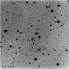 |
Fig. 1 Finding chart with the position of MN Dra marked as V1 and two comparison stars C1 and C2. The field of view is about 6.5′ × 6.5′. |
3. Light curves
3.1. Global photometric behaviour
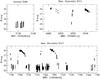 |
Fig. 2 Global photometric behaviour of MN Dra. |
For convenience, we use only a day number HJD-2 450 000 [d] to refer to our observations. Figure 2 shows the light curves of MN Dra during our three campaigns.
At the time of observations in 2009 (top left panel of Fig. 2), MN Dra was in quiescence, but we detected negative superhumps (more in Sects. 3.4 and 3.5).
During the 2013 campaigns (Fig. 2, top right panel), we observed two superoutbursts interspersed with one normal outburst. Because of unfavourable weather conditions, we obtained only four nights of data covering the first July 2013 superoutburst HJD 6482, 6483, 6492, and 6495. However, clear superhumps were observed on HJD 6483. Later on, MN Dra was caught on the rise to normal outburst during the HJD 6517, 6518, and 6519 nights. The last data from the 2013 campaign containing seven nights (between HJD 6539 and HJD 6546) showed the object in the September 2013 superoutburst. At this time, the superhumps were also clearly visible in each run.
During the 2015 campaign (bottom panel), we gathered 14 nights (HJD 7199–7212) of the June–July superoutburst and 13 nights (between HJD 7268 and HJD 7286) of the September superoutburst. Additionally, we detected three normal outbursts that occurred in June, August, and December 2015.
During maximum brightness, MN Dra reached R ≈ 15.7 mag, and after its superoutbursts, the star faded to R ≈ 18.6 mag, resulting in an average amplitude of the superoutburst of As ≈ 2.9 mag. In quiescence, the brightness of MN Dra varied between R ≈ 18.4 and R ≈ 20.3 mag. Because of diverse weather during several normal outbursts, no estimates of outburst amplitudes and their maximum and minimum levels were possible.
3.2. Supercycle length
The supercycle length of MN Dra has been measured twice so far. The first measurement, Psc1 ~ 60 days, was derived by Nogami et al. (2003), with no uncertainty given.
The second estimation was made by Samsonov et al. (2010). They reported the length of the supercycle as ~30 days. Nonetheless, based on the visual inspection of the light curve presented in Fig. 1 (Samsonov et al. 2010), we consider this value to be completely incorrect. Hence, we reanalysed the supercycle length and obtained a rough estimate of Psc2 ~ 67.5 ± 2.5 days.
We derived Psc3 from our data from 2015, using the ANOVA code of (Schwarzenberg 1996). The most prominent peak of the power spectrum was found at the frequency 0.0135(1) [c/d], and this corresponds to Psc3 = 74 ± 0.5 days.
Because our estimate of Psc3 is based on only two superoutbursts observed in 2015, we decided to investigate our result more precisely. First, we looked for amateur data of MN Dra in superoutbursts in databases such as the AAVSO1, which covers the 2014 − 2016 observational seasons. Unfortunately, this object was not observed by amateurs. Without any additional observations, we decided to calculate the supercycle length based on our data set covering all four superoutbursts we detected in the 2013 and 2015 observational campaigns. We obtained a supercycle period of ~72 days. Not only does this crude estimate confirm that the supercycle length of MN Dra is constantly increasing, but it also shows that the time span between two successive superoutbursts is currently longer than 72 days. Including our data set, the corresponding increasing rate of the supercycle length is ˙P = 3.3 × 10⁻³. Therefore, we consider Psc3 = 74 ± 0.5 days as reasonable and the best current value of the supercycle length of MN Dra.
It is worth noting that the light curves covering subsequent superoutbursts presented by Nogami et al. (2003) and Samsonov et al. (2010) have significant gaps, in particular, they lack the beginnings or ends of the superoutbursts. We therefore tested the values of the supercycle length one more time. This time we calculated the time span between the last nights of quiescence between subsequent superoutbursts. Moreover, we derived the time span between the first nights of the quiescence after superoutbursts. Based on this analysis, the supercycle lengths were found to be Psc1b = 62 days for the data set presented by Nogami et al. (2003) and Psc2b = 68 days for the light curves given by Samsonov et al. (2010). With our data set, the rate of the increase in supercycle length was ˙P = 2.8 × 10⁻³.
In Fig. 3 we present all available measurements of Psc. The black line represents the fit calculated based on Psc1, Psc2, and Psc3 days. The dotted line corresponds to the fit obtained based on Psc1b, Psc2b, and Psc3 days. In both cases, the immediate conclusion is that the supercycyle length of MN Dra has increased during the past twelve years. The corresponding rate of the increase in period is ˙P = 2.8 − 3.3 × 10⁻³.
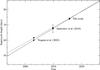 |
Fig. 3 Increasing supercycle length of MN Dra during the past twelve years. Lines correspond to the best fits to the data (details in text). Uncertainties are given when available. The value of the supercycle length (Samsonov et al. 2010) was calculated by the authors of this work based on the light curves presented in Samsonov et al. (2010). |
The period Psc3 was used to create the folded light curve of the June–July 2015 and the September 2015 superoutbursts in MN Dra. The result is presented in Fig. 4.
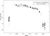 |
Fig. 4 Light curve of MN Dra during superoutbursts folded with Psc = 74 days. Black circles correspond to the June–July 2015 superoutburst, and grey circles represent the September 2015 superoutburst. |
3.3. Superhumps
In the light curves of MN Dra clear superhumps are visible. Examples of these characteristic “tooth-shaped” oscillations are presented in Figs. 5–7 during superoutburts, normal outbursts, and in quiescence, respectively.
We performed power spectra and an O−C analysis for the detected periodicities. The following sections present the results of this investigation.
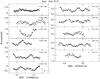 |
Fig. 5 Light curves of MN Dra during the June–July 2015 superoutburst. A fraction of HJD is presented on the x-axis. HJD-2 450 000 [d] is given at the right side of each panel. |
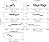 |
Fig. 6 Light curves of MN Dra during its normal outbursts observed in August 2013, June 2015, August 2015, and December 2015. |
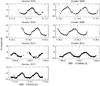 |
Fig. 7 Light curves of MN Dra in quiescence. The October 2009 data set was obtained with the 1.3-m telescope in Greece. The October 2015 observations were gathered with the 1.3-m telescope located in the USA. |
3.4. Period analysis
We detrended the light curves of MN Dra by subtracting first- or second-order polynomials. Data from each observatory and from each night were converted one at a time. Then, we analysed them using the ANOVA statistics with one or two harmonic Fourier series (Schwarzenberg 1996).
Because of the different levels of quality of the collected data and various types of periodicities, we investigated them separately. Our data were divided into six sets:
-
the September 2013 superoutburst;
-
the June–July 2015 superoutburst;
-
the September 2015 superoutburst;
-
normal outbursts;
-
the October 2009 quiescence;
-
the October 2015 quiescence.
3.4.1. Superoutbursts
For the September 2013 and the June–July 2015 superoutbursts the most prominent peak was found at the frequency fsh1 = 9.510(7) [c/d] and fsh2 = 9.510(10) [c/d], respectively. This corresponds to a period Psh1 = 0.10515(8) days and Psh2 = 0.10515(11) days. In case of the September 2015 superoutburst, the highest peak was detected at the frequency fsh3 = 9.300(90) [c/d], which determines the period of Psh3 = 0.10753(104) days.
We adopt Psh1 = Psh2 as the superhump period of MN Dra. Not only has it appeared in two superoutbursts with the exact same value, but the time coverage of the observations collected during the September 2015 superoutburst was also worse than for the September 2013 and the June–July 2015 superoutbursts.
The pre-whitening procedure of the detrended light curves was performed to search for additional periodicities. We removed the modulation of the superhump period and then conducted the ANOVA analysis. The resulting power spectra have intricate structures in all three cases of investigated superoutbursts. Although we scrutinized several peaks in prewhitened spectra, we did not find any physical explanation of their presence.
Figure 8 shows the power spectra for the light curves of the superoutbursts in September 2013 (top panel), June–July 2015 (middle panel), and September 2015 (bottom panel) in MN Dra. Figure 9 presents periodograms for pre-whitened light curves of the superoutbursts in September 2013 (top), June–July 2015 (middle), and September 2015 (bottom) in MN Dra.
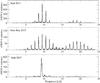 |
Fig. 8 ANOVA power spectra of the light curves of MN Dra during the superoutbursts in September 2013, June–July 2015, and September 2015. |
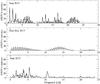 |
Fig. 9 ANOVA power spectra of the pre-whitened light curves of MN Dra during the superoutbursts in September 2013, June–July 2015, and September 2015. |
3.4.2. Normal outbursts
Because the weather was poor during every normal outburst, we were unable to investigate these outbursts separately. Based on the all collected data, presented in Fig. 6, we performed the power spectra analysis. Figure 10 presents the resulting periodogram with the two highest peaks located at frequencies 10.530(3) [c/d] and 11.400(5) [c/d], respectively. However, we can only interpret the first value fnsh1 = 10.530(3) [c/d] as the corresponding to the negative superhump period Pnsh1 = 0.09497(3) days. Figure 11 shows the outcome of the pre-whitening analysis. Again, we interpret the detected peaks as probably false signals.
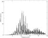 |
Fig. 10 ANOVA power spectra of the light curves of MN Dra during its normal outbursts. |
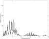 |
Fig. 11 ANOVA power spectra of the pre-whitened light curves of MN Dra during its normal outbursts. |
3.4.3. Quiescence
The best-quality data of MN Dra at minimum brightness were gathered on 1.3-m telescopes located in Greece and in the USA (Table 1 and Fig. 7). Hence, we performed two separate power spectra analyses for data sets covering light curves collected in October 2009 in Crete and in October 2015 in Arizona.
The top left panel of Fig. 12 shows the resulting power spectrum of the light curves from the October 2009 data set. The most prominent frequency was detected at fnsh2 = 10.500(2) [c/d], and it is associated with the negative superhump period Pnsh2 = 0.09524(2) days. The harmonic analysis-of-variance periodogram for pre-whitened light curves of MN Dra collected in Greece is presented in the top right panel of Fig. 12. This forest of frequencies is caused by the changes in amplitude and the period of negative superhumps. The occurrence of negative humps is not a strictly periodic phenomenon, and hence it is impossible to subtract its value with only one analytical fit. As a result, we observe residua on the lower frequencies in the periodogram.
The result of the investigation of the October 2015 light curves based on the ANOVA statistics is displayed in the left bottom panel of Fig. 12. This time, the highest signal was found at fnsh3 = 10.470(6) [c/d] corresponding to Pnsh3 = 0.09551(6) days. In the pre-whitened spectra, presented in the right bottom panel of Fig. 12, we detected the highest signal at f = 3.360(10) [c/d]. Despite our efforts, we have no physical interpretation for the detected frequency.
In Table 2 we present the detected periodicities in the light curves of MN Dra during its superoutbursts, normal outbursts, and in quiescence.
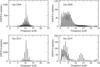 |
Fig. 12 ANOVA power spectra of the light curves (left panels) and pre-whitened light curves (right panels) of MN Dra during quiescence. |
3.5. O−C diagram for superhumps
We observed positive and negative superhumps in the light curves of MN Dra. To check the stability of the detected oscillations, an O−C analysis for these periodicities was performed.
3.5.1. Superoutbursts
Here, we present results only for the September 2013 and the June–July 2015 superoutbursts. Owing to unfavourable weather conditions, the September 2015 data were scattered and of a lower quality than the observations collected during the September 2013 and the June–July 2015 superoutbursts.
We identified 16 moments of maxima in the light curves of MN Dra during its September 2013 superoutburst. A linear fit allowed us to obtain the following ephemeris:  (1)Additionally, the second-order polynomial fit was calculated for the moments of maxima, and the corresponding ephemeris was obtained as
 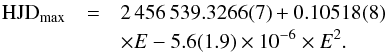 (2)In the data set of the June–July 2015 superoutburst, we determined 9 peaks of maxima. The following ephemeris was derived as
  (3)Once again, we calculated the second-order polynomial fit for the moments of maxima, and we obtained
 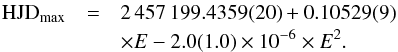 (4)Based on the derived ephemerides presented in Eqs. (1) and (3), the corresponding superhump periods were obtained as Psh4 = 0.10496(2) days (151.1424 ± 0.03 min) and Psh5 = 0.10512(3) days (151.3728 ± 0.04 min) for the September 2013 and the June–July 2015 superoutbursts, respectively.
Tables 3 and 4 list cycle numbers E, times of detected maxima, errors, hump amplitudes, and the O−C values for the September 2013 and the June–July 2015 superoutbursts, respectively.
Most prominent frequencies detected in the light curves of MN Dra.
Figures 13 and 14 show light curves of MN Dra during its superoutbursts (top panels), evolution of amplitudes of humps (middle panels), and the O−C diagrams for detected maxima (bottom panels).
We display the O−C values corresponding to the two analysed superoutbursts from September 2013 and June–July 2015 in Figs. 15 and 16, respectively. Atmospheric conditions allowed us to obtain better coverage of the first part of the September 2013 superoutburst and the second part of the June–July 2015 superoutburst. In the September 2013 data, most of the moments of maxima were therefore detected between 0 and 40 cycles, and for the June–July 2015 set between 40 and 90 cycles.
In Table 5 we present the superhump periods of MN Dra that have been calculated so far. As described, we derived the second-order polynomial fit (black curves in Figs. 15 and 16). However, in both cases the error of square factor E2 in Eqs. (2) and (4) is substantial enough for us to postulate that there is a poor agreement between the second-order polynomial fit and the O−C values of the moments of maxima. Therefore, we cannot confirm the values of increasing or decreasing trends of the superhump period postulated by Nogami et al. (2003), Pavlenko et al. (2010), Samsonov et al. (2010). We also question the value given by Kato et al. (2014b) because its error is enormous.
Times of superhump maxima of MN Dra during its 2013 September superoutburst.
Times of superhump maxima of MN Dra during its 2015 June–July superoutburst.
 |
Fig. 13 Light curves of MN Dra during the September 2013 superoutburst (top panel), the evolution of the amplitude of superhumps (middle panel), and the O−C diagram for the superhump maxima (bottom panel). |
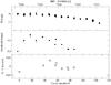 |
Fig. 14 Light curves of MN Dra during the June–July 2015 superoutburst are shown in the top panel. The evolution of the amplitude of superhumps is presented in the middle panel. In three cases of scattered and/or incomplete data, the arrow marks a rough estimate of the amplitude, which is larger than the value indicated by a corresponding black circle. The O−C diagram for the superhumps maxima is in the bottom panel. |
3.5.2. Normal outbursts
We performed the O−C analysis for two sets of observations covering normal outbursts that occurred in June 2015 and in August 2015.
During each normal outburst in MN Dra, we collected data during two subsequent nights and identified four moments of maxima. All determined peaks of maxima, together with their errors, cycle numbers E, and the O−C values are listed in Table 6.
From a linear fit, we calculated the following ephemerides: 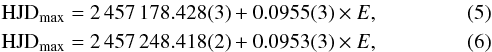 and these values correspond to the negative superhump periods of Pnsh4 = 0.0955(3) days (137.52 ± 0.4 min) and Pnsh5 = 0.0953(3) days (137.23 ± 0.4 min) for the June 2015 and the August 2015 normal outbursts in MN Dra, respectively.
Figure 17 displays the O−C values corresponding to the ephemerides given by Eqs. (5) and (6).
Values of superhump periods of MN Dra form 2002 until 2015.
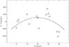 |
Fig. 15 O−C diagram for the September 2013 superoutburst in MN Dra with the second-order polynomial fit (black curve). |
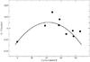 |
Fig. 16 O−C diagram for the June–July 2015 superoutburst in MN Dra with the second-order polynomial fit (black curve). |
3.5.3. Quiescence
Furthermore, the O−C diagrams were constructed for two campaigns conducted in October 2009 and in October 2015 while MN Dra was in quiescent state.
Once again, in Table 7 we present the HJD times of detected moments of maxima, errors, number of cycles E, and the O−C computed according to the linear ephemerides presented below: 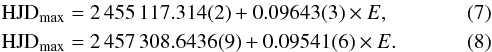 and associated with the negative superhump periods of Pnsh6 = 0.09643(3) days (138.8592 ± 0.04 min) and Pnsh7 = 0.09541(6) days (137.3904 ± 0.09 min) for the October 2009 and the October 2015 light curves of MN Dra in quiescence, respectively.
In Table 8 we present detected periods, from the O−C analyses, in the light curves of MN Dra during its normal outbursts and in quiescence. Differences between the values of Pnsh presented in Table 8 exceed 3σ. This indicates that the negative superhump period of MN Dra is not stable. The mechanism responsible for negative superhumps is probably a classical regression of the tilted disk. Therefore, in the case of MN Dra, the period of the regression of the accretion disk is also changing.
The O−C values corresponding to the ephemerides given by Eqs. (7) and (8) are presented in Fig. 18.
Times of negative superhump maxima of MN Dra during its normal outbursts in June and August 2015.
4. Discussion
4.1. Supercycle length
The supercycle lengths of several very active DN below the period gap have been analysed by Otulakowska-Hypka et al. (2013) and Otulakowska-Hypka & Olech (2013). They showed observational evidence that the supercycle lengths of the investigated systems have been increasing as a result of their mean mass-transfer rates, which have been constantly decreasing. Therefore, they examined this phenomenon in the context of the future evolution of DN. With the assumption that the supercycle length will be increasing in the same way in the future, they estimated the timescale of the next steps of the evolution of ER UMa objects to become SU UMa and WZ Sge-type systems (see Table 3 in Otulakowska-Hypka & Olech 2013). These predictions are in agreement with results presented by Patterson et al. (2013) concerning the BK Lyn evolution. According to Patterson et al. (2013), BK Lyn, which is a member of ER UMa group today, is in a transient stage of evolution, preceded by the classical nova and nova-like variable phases. If this hypothesis is true for all active SU UMa systems, it means all these objects are survivors of classical nova eruptions that have been fading ever since.
The changes in supercycle length of MN Dra are the same as the behaviour of several cases of DN below the period gap presented by Otulakowska-Hypka et al. (2013) and Otulakowska-Hypka & Olech (2013). Therefore, we discovered the first period-gap object in which the occurrence of superoutbursts has been constantly decreasing within the past decades.
4.2. Orbital period determination
We used the latest version of the Stolz and Schoembs relation (Otulakowska-Hypka et al. 2016): ![Mathematical equation: \begin{equation} {\rm log }\: \varepsilon = 1.97 (0.10) \times {\rm log}\: P_{\rm orb}\: {\rm [d]} + 0.73(0.11), \end{equation}](/articles/aa/full_html/2017/07/aa30375-16/aa30375-16-eq115.png) (9)and the following formula defining the superhump period excess/deficit as
(9)and the following formula defining the superhump period excess/deficit as  (10)to estimate the orbital period Porb = 0.0994(1) days (143.126 ± 0.144 min) and the period excess ε = 5.7% ± 0.1% and deficit ε− = 2.5% ± 0.6% and their ratio φ = − 0.44(11) for MN Dra.
Knowing ε and Porb, we were able to determine the evolutionary status of DN, since the mass ratio decreases with time due to the mass-loss from the secondary. In Fig. 19 the small open circles represent known DN (from Olech et al. 2011) and black squares correspond to systems with known supercycle lengths (from Otulakowska-Hypka & Olech 2013). The position of MN Dra is marked with a black cross.
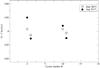 |
Fig. 17 O−C diagram for the June 2015 (open circles) and the August 2015 (black circles) normal outbursts in MN Dra. |
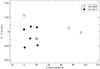 |
Fig. 18 O−C diagram for the October 2009 (open circles) and the October 2015 (black circles) data sets of MN Dra in quiescence. |
Times of negative superhump maxima of MN Dra during quiescence in October 2009 and October 2015.
Values of negative superhump periods of MN Dra from 2002 until 2015.
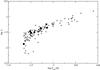 |
Fig. 19 Relation between the period excess and the orbital period for DN. Small open circles represent known DN (Olech et al. 2011). Black squares correspond to the position of active systems for which the supercycle lengths were calculated (Otulakowska-Hypka & Olech 2013). The position of MN Dra is marked with a black cross. |
Retter et al. (2002) suggested that there is a correlation between φ and Porb for CVs that exhibit both positive and negative superhumps, and Olech et al. (2009) presented the following empirical formula for this dependency: ![Mathematical equation: \begin{equation} \phi = 0.318(6) \times {\rm log}\:P_{\rm orb}\: {\rm [d]} - 0.161(10). \end{equation}](/articles/aa/full_html/2017/07/aa30375-16/aa30375-16-eq128.png) (11)We can confirm their hypothesis for the case of MN Dra. Figure 20 presents the relation between the ratio φ and orbital period for several CVs including MN Dra.
(11)We can confirm their hypothesis for the case of MN Dra. Figure 20 presents the relation between the ratio φ and orbital period for several CVs including MN Dra.
Next, by employing an empirical formula for the relation between the period excess and the mass ratio of the binary q = M2/M1 (Patterson 1998),  (12)we derived the mass ratio for MN Dra as equal to q ≈ 0.26. It is worth mentioning that Kato et al. (2014b) obtained a similar result of q = 0.258 based on the orbital period calculated by Pavlenko et al. (2010).
4.3. Superhumps
4.3.1. Active period-gap DN
In CVs with long orbital periods, magnetic braking is the dominant mechanism for angular momentum loss. It is thought that around Porb ⋍ 3 h the secondary becomes fully convective (Verbunt & Zwaan 1981) and causes the termination of magnetic braking. In response, the secondary contracts and detaches from its Roche lobe. At this point, the cataclysmic system is a detached binary of low luminosity. As a result of the continuous loss of orbital angular momentum, the orbit decays, and this results in the re-establishment of contact at a period of ~2 h. Hence, the mass transfer is resumed, and both its loss and its rate are driven by gravitational radiation. The system re-emerges as an active CV at the bottom of the period gap. Knigge (2006) revisited the estimation of the period gap and presented its new localisation at 3.18(0.04) ≤ Porb ≤ 2.15(0.03) h.
Even though the explanation outlined above seems satisfactory for the significant dearth of CVs in the period range 2 ≲ Porb ≲ 3 h (Gänsicke et al. 2009), there are still many missing pieces in this puzzle. SU UMa systems located in the period gap are expected to have neither significant magnetic breaking nor significant angular momentum loss from gravitational radiation. Therefore these objects should be characterised by low activity. Hence, among the challenges open to interpretation are the recent discoveries of active DN with orbital periods within period gap, such as TU Men (Stolz & Schoembs 1981), SDSS J162520.29+120308.8 (Olech et al. 2011), OGLE-BLG-DN-001 (Poleski et al. 2011), CzeV404 (Bąkowska et al. 2014), or NY Ser (Pavlenko et al. 2014). Taking into account that MN Dra has an orbital period within the period gap range (Porb ~ 2.38 h) and shows rapid superoutburst activity (Psc ~ 74 days), this DN is the latest observational evidence contradicting the existing theory of the evolution of CVs.
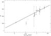 |
Fig. 20 Relation between the ratio between period deficit and excess and orbital period of different types of CVs. The position of MN Dra is marked by the black triangle. Figure taken from Olech et al. (2009). |
4.3.2. Positive superhumps
To verify whether the rate of Ṗsignificantly changes from epoch to epoch, we investigated all published O-C diagrams of positive superhumps in MN Dra. Our conclusion is that during most of the superoutbursts, MN Dra shows smooth changes of superhump period and rather small or standard negative superhump period derivatives. Frequently, the O−C diagrams look rather flat during the whole superoutburst (see Fig. 6 in Nogami et al. 2003; and Fig. 2 in Samsonov et al. 2010).
Kato et al. (2009, 2010, 2012, 2013, 2014a,b, 2016a) published a comprehensive survey of period variations of superhumps in SU UMa-type DN. According to this, the evolution of the superhump period can typically be divided into three separate parts: the first stage (A) corresponds to a presence of early superhumps with a stable and longer period, the middle stage (B) refers to a positive superhump period derivative, and the final stage (C) is characterised by a shortened but again stable superhump period. According to Kato et al. (2009), in the well-observed DN, the transition between stages A and B and stages B and C is abrupt and discontinuous. There are examples of SU UMa period-gap objects following this scenario, for instance, V1006 Cyg (Kato et al. 2016c) and SDSS J162520.29+120308.8 (Olech et al. 2011). However, Olech et al. (2003) showed that these transitions can be also smooth changes. In case of MN Dra, Kato et al. (2014b) presented the transition between stages A and B for several superoutbursts (see Fig. 19 in Kato et al. 2014b) and concluded that the superhump period of MN Dra is characterised by a large negative .Ṗ Nonetheless, in the O−C diagrams constructed from our data sets, we did not detect stage A of MN Dra during any of its superoutbursts. Moreover, it seems that a lack of significant or abrupt changes in superhump period in MN Dra is not peculiar. There are cases of DN that display rather small changes in superhump derivatives and the shapes of their O−C diagrams are rather flat, such as RZ LMi (Fig. 2 in Kato et al. 2016b), V452 Cas (Fig. 6 in Kato et al. 2014b), or GZ Cnc (Fig. 11 in Kato et al. 2014b). Hence, the observed behaviour of MN Dra is in agreement with theory, which interprets negative superhumps period derivatives in the O−C diagrams as a result of the disk shrinkage during the superoutburst and thus lengthening its precession rate (Lubow 1991; Patterson 1998).
4.3.3. Negative superhumps
CVs with negative superhump manifestations are detected rarely. At present, we know of roughly a dozen confirmed cases (see Table 2 in Montgomery 2009; Table 5 in Armstrong et al. 2013). Unlike positive superhump theory, no consensus about the source of negative superhump has been established as yet. Possible mechanisms responsible for negative superhumps and challenges open for interpretation can be found in Montgomery (2009).
In case of MN Dra, negative superhumps were investigated during normal outbursts by Samsonov et al. (2010) and Pavlenko et al. (2010). They noted that the maxima of negative superhumps varied cyclically in correlation with normal outbursts (Figs. 5 and 6 in Samsonov et al. 2010; Fig. 5 in Pavlenko et al. 2010). Based on our results, we cannot confirm this correlation. However, it must be noted that our sets of data, gathered during normal outbursts in MN Dra, are scattered and insufficient for any conclusive remarks.
According to Patterson et al. (1997), negative superhumps are associated with retrograde precession and are not strictly periodic. For example, these signals are present during several months of observations, they cannot be detected a year later, and finally, they reappear several years after that. In this context, a disk can remain stably tilted for some time, later on the disk realigns with the orbital plane and maintains this position for another period of time, then it returns to its previous tilted position. Nonetheless, the problem of how a disk initially tilts remains unsolved. MN Dra probably follows this scenario. We did not detect any changes in the negative superhump periods on short timescales of days and months during normal outbursts and during quiescence. That is why our O−C diagrams were rather flat. However, we noted the differences between the values of Pnsh from 2009 and 2015, which exceed 3σ. This shows that the negative superhump period of MN Dra is not stable on longer timescales of years. Hence, it is probable that the mechanism responsible for negative superhumps is a classical regression of the tilted disk.
It is worth noting that our observational results of the period excess, period deficit, and mass ratio of MN Dra are in agreement with the recent smoothed particle hydrodynamics simulations performed by Thomas & Wood (2015; see Fig. 9). Therefore, MN Dra is an excellent object to thoroughly test the hypothesis of the tilted-disk geometry as the source of negative superhumps, but most importantly, to test the theory that invokes white-dwarf magnetism to break the azimuthal symmetry and permits creating the disk tilt postulated by Thomas & Wood (2015).
5. Conclusions
To conclude, we present a summary of our world-wide observational campaign of MN Dra.
-
MN Dra was observed during three campaigns in 2009, 2013, and 2015. We detected MN Dra in a quiescent state during six nights of observations in October 2009. At the time of our second campaign, between June and September 2013, the star was monitored during two superoutbursts interspersed with one normal outburst. In our most recent campaign, from June to December 2015, two superoutbursts and three normal outbursts in MN Dra were recorded. The average amplitude of brightness during superoutbursts was As ≈ 2.9 mag. We detected clear positive superhumps during superoutburts. In addition, negative superhumps were observed in this DN during its normal outbursts and in quiescence. The duration of a superoutburst was on average 24 ± 1 days.
-
The supercycle length, with a value of Psc = 74 ± 0.5 days, was derived for the two subsequent superoutbursts observed in June–July 2015 and in September 2015. Based on our data set and observations presented by Nogami et al. (2003) and Samsonov et al. (2010), the supercycle length has been increasing during the past twelve years with a rate of ˙P = 3.3 × 10⁻³. Additionally, the occurrence of superoutbursts observed in MN Dra follows the scenario presented in Otulakowska-Hypka et al. (2013) and Otulakowska-Hypka & Olech (2013) for very active ER UMa stars. MN Dra is also the first discovered SU UMa system in the period gap with increasing supercycle length, and therefore it is crucial for our understanding of the future evolution of DN.
-
We conducted an O−C analysis for the moments of maxima detected in the September 2013 and the June–July 2015 superoutbursts in MN Dra, and the superhump period was Psh4 = 0.10496(2) days (151.1424 ± 0.03 min) and Psh5 = 0.10512(3) days (151.3728 ± 0.04 min), respectively. We also calculated the second-order polynomial fit. Nonetheless, because of the poor agreement between the fit and the O−C values of the moments of maxima, we cannot confirm the changes in trend of the superhump period postulated by Nogami et al. (2003), Samsonov et al. (2010) or Pavlenko et al. (2010).
-
To investigate the negative humps in MN Dra, we used our best-quality observations obtained in October 2009 and in October 2015 on the 1.3-m telescopes located in Greece and in the USA, respectively. The negative superhump period was obtained with a value of Pnsh6 = 0.09643(3) days (138.8592 ± 0.04 min) and Pnsh7 = 0.09541(6) days (137.3904 ± 0.09 min) for the 2009 and the 2015 data, respectively.
-
We derived the period excess and the period deficit ε = 5.7% ± 0.1% and ε− = 2.5% ± 0.6%, respectively. We also obtained the orbital period with a value of Porb = 0.0994(1) days (143.126 ± 0.144 min). In the diagram Porb versus ε, MN Dra is located in the range of the period-gap objects.
-
We obtained the mass ratio with a value of q ≈ 0.26, which is in accordance with one of the values, q = 0.258, obtained by Kato et al. (2014b).
MN Dra is another example of an active DN located in the period gap (Bąkowska et al. 2014). It is worth noting that this star is not only a challenge for existing models of the superhump and superoutburst mechanisms, but also presents other intriguing behaviours, in particular the increasing supercycle length. Moreover, we know only a few DN that exhibit positive and negative superhumps (see Retter et al. 2002; Olech et al. 2009), and there are the only two known cases of period-gap SU UMa objects showing negative superhumps (Pavlenko 2016). Hence, MN Dra is a perfect object for further photometric observations, that is, a good light curve coverage in normal outbursts would allow to determine normal cycle length and determine its stability. To conclude, we presented a new set of information about MN Dra and also updated available basic statistics of the system, that is, the orbital period, where we used indirect methods different than Pavlenko et al. (2010) for its determination.
We emphasize the lack of spectroscopic analysis of this object, which could provide many answers regarding this type of very active period-gap system. However, the very low (below 18 mag) brightness in quiescence of MN Dra, located on the northern sky, poses a challenge for spectroscopic observations.
American Association of Variable Star Observers, \http:www.aavso.org
Acknowledgments
This work is partially based on observations obtained at the MDM Observatory, operated by Dartmouth College, Columbia University, Ohio State University, Ohio University, and the University of Michigan. K.B. wishes to thank K. Z. Stanek and E. Galayda for the generous allocation of time at the 1.3-m telescope and the technical support in MDM Observatory. We are indebted to the anonymous referee of an earlier version of this paper for providing insightful comments and providing directions for additional work, which has resulted in this paper. The project was supported by the Polish National Science Center grants awarded by decisions DEC-2012/07/N/ST9/04172 and DEC-2015/16/T/ST9/00174 for K.B.
References
- Armstrong, E., Patterson, J., Michelsen, E., et al. 2013, MNRAS, 435, 707 [NASA ADS] [CrossRef] [Google Scholar]
- Bąkowska, K., & Olech, A. 2014, Acta Astron., 64, 247 [NASA ADS] [Google Scholar]
- Bąkowska, K., Olech, A., Pospieszyński, R., et al. 2014, Acta Astron., 64, 337 [NASA ADS] [Google Scholar]
- Barrett, P., O’Donoghue, D., & Warner, B. 1988, MNRAS, 233, 759 [NASA ADS] [CrossRef] [Google Scholar]
- Cannizzo, J. K. 1993, ApJ, 419, 318 [NASA ADS] [CrossRef] [Google Scholar]
- Cutri, R. M., Skrutskie, M. F., van Dyk, S., et al., 2003, VizieR Online Data Catalog: II/246 [Google Scholar]
- Gänsicke, B. T., Dillon, M., Southworth, J., et al. 2009, MNRAS, 397, 2170 [NASA ADS] [CrossRef] [Google Scholar]
- Hellier, C. 2001, Cataclysmic Variable Stars (Springer) [Google Scholar]
- Hirose, M., & Osaki, Y. 1990, PASJ, 42, 135 [NASA ADS] [Google Scholar]
- Kato, T., Imada, A., Uemura, M., et al. 2009, PASJ, 61, 395 [NASA ADS] [Google Scholar]
- Kato, T., Maehara, H., Uemura, M., et al. 2010, PASJ, 62, 1525 [NASA ADS] [Google Scholar]
- Kato, T., Maehara, H., Miller, I., et al. 2012, PASJ, 64, 21 [NASA ADS] [Google Scholar]
- Kato, T., Hambsch, F.-J., Maehara, H., et al. 2013, PASJ, 65, 23 [NASA ADS] [CrossRef] [Google Scholar]
- Kato, T., Hambsch, F.-J., Maehara, H., et al. 2014a, PASJ, 66, 30 [NASA ADS] [Google Scholar]
- Kato, T., Dubovsky, P. A., Kudzej, I., et al. 2014b, PASJ, 66, 90 [NASA ADS] [Google Scholar]
- Kato, T., Hambsch, F.-J., Monard, B., et al., 2016a, PASJ, 68, 65 [NASA ADS] [Google Scholar]
- Kato, T., Ishioka, R., Isogai, K., et al., 2016b, PASJ, 68, 107 [NASA ADS] [Google Scholar]
- Kato, T., Pavlenko, E. P., Shchurova, A. V., et al., 2016c, PASJ, 68, L4 [NASA ADS] [Google Scholar]
- Knigge, C. 2006, MNRAS, 373, 484 [NASA ADS] [CrossRef] [Google Scholar]
- Lasota, J.-P. 2001, New Astron. Rev., 45, 449 [NASA ADS] [CrossRef] [Google Scholar]
- Lubow, S. H. 1991, ApJ, 381, 268 [NASA ADS] [CrossRef] [Google Scholar]
- Montgomery, M. M. 2009, MNRAS, 394, 1897 [NASA ADS] [CrossRef] [Google Scholar]
- Nogami, D., Uemura, M., Ishioka, R., et al. 2003, A&A, 404, 1067 [NASA ADS] [CrossRef] [EDP Sciences] [Google Scholar]
- Olech, A., Schwarzenberg-Czerny, A., Kędzierski, P., et al. 2003, Acta Astron., 53, 175 [NASA ADS] [Google Scholar]
- Olech, A., Rutkowski, A., & Schwarzenberg-Czerny, A. 2009, MNRAS, 399, 465 [NASA ADS] [CrossRef] [Google Scholar]
- Olech, A., de Miguel, E., Otulakowska, M., et al., 2011, A&A, 532. A64 [NASA ADS] [CrossRef] [EDP Sciences] [Google Scholar]
- Otulakowska-Hypka, M., & Olech, A. 2013, MNRAS, 433, 1338 [NASA ADS] [CrossRef] [Google Scholar]
- Otulakowska-Hypka, M., Olech, A., de Miguel, E., et al. 2013, MNRAS, 429, 868 [NASA ADS] [CrossRef] [Google Scholar]
- Otulakowska-Hypka, M., Olech, A., & Patterson, J. 2016, MNRAS, 460, 2526 [NASA ADS] [CrossRef] [Google Scholar]
- Osaki, Y. 1985, A&A, 144, 369 [NASA ADS] [Google Scholar]
- Osaki, Y. 1989, PASJ, 41, 1005 [NASA ADS] [Google Scholar]
- Osaki, Y. 1996, PASP, 108, 39 [NASA ADS] [CrossRef] [Google Scholar]
- Patterson, J. 1998, PASP, 110, 1132 [NASA ADS] [CrossRef] [Google Scholar]
- Patterson, J., Kemp, J., Shambrook, A., et al. 1997, PASP, 109, 1100 [NASA ADS] [CrossRef] [Google Scholar]
- Patterson, J., Uthas, H., Kemp, J., et al. 2013, MNRAS, 434, 1902 [NASA ADS] [CrossRef] [Google Scholar]
- Pavlenko, E. 2016, in 41st COSPAR Scientific Assembly Abstracts [Google Scholar]
- Pavlenko, E. P., Voloshina, I. B., Andreev, M. V., et al. 2010, Astron. Rep., 54, 6 [NASA ADS] [CrossRef] [Google Scholar]
- Pavlenko, E. P., Kato, T., Sosnovskij, A. A., et al. 2014, PASJ, 66, 111 [NASA ADS] [Google Scholar]
- Poleski, R., Soszyński, I., Udalski, A., et al. 2011, Acta Astron., 61, 123 [NASA ADS] [Google Scholar]
- Retter, A., Chou, Y., Bedding, T. R., et al. 2002, MNRAS, 330, L37 [NASA ADS] [CrossRef] [Google Scholar]
- Samsonov, D. A., Pavlenko, E. P., Andreev, M. V., et al. 2010, Odessa Astron. Publ., 23, 98 [NASA ADS] [Google Scholar]
- Schwarzenberg-Czerny, A. 1996, ApJ, 460, L107 [NASA ADS] [CrossRef] [Google Scholar]
- Smak, J. 1984, PASP, 96, 5 [NASA ADS] [CrossRef] [Google Scholar]
- Smak, J. I. 1991, Acta Astron., 41, 269 [NASA ADS] [Google Scholar]
- Smak, J. 1996, in Cataclysmic Variables and Related Objects, IAU Colloq. 158, Astrophys. Space Sci. Lib., 208, 45 [NASA ADS] [CrossRef] [Google Scholar]
- Smak, J. 2000, New Astron. Rev., 44, 171 [Google Scholar]
- Smak, J. 2008, Acta Astron., 58, 65 [NASA ADS] [Google Scholar]
- Stetson, P. B. 1987, PASP, 99, 191 [NASA ADS] [CrossRef] [Google Scholar]
- Stolz, B., & Schoembs, R. 1981, IBVS, 1955 [Google Scholar]
- Thomas, D. M., & Wood M. A. 2015, ApJ, 803, 55 [NASA ADS] [CrossRef] [Google Scholar]
- Verbunt, F., & Zwaan, C. 1981, A&A, 100, L7 [NASA ADS] [Google Scholar]
- Vogt, N. 1982, ApJ, 252, 653 [NASA ADS] [CrossRef] [Google Scholar]
- Vogt, N. 1983, A&A, 118, 95 [NASA ADS] [Google Scholar]
- Warner, B. 1995, Cataclysmic variable stars, Cambridge Astrophys. Ser., 28 [Google Scholar]
- Whitehurst, R. 1988, MNRAS, 232, 35 [NASA ADS] [Google Scholar]
- Wood, M. A., & Burke, C. J. 2007, ApJ, 661, 1042 [NASA ADS] [CrossRef] [Google Scholar]
All Tables
Times of negative superhump maxima of MN Dra during its normal outbursts in June and August 2015.
Times of negative superhump maxima of MN Dra during quiescence in October 2009 and October 2015.
All Figures
|
Fig. 1 Finding chart with the position of MN Dra marked as V1 and two comparison stars C1 and C2. The field of view is about 6.5′ × 6.5′. |
| In the text | |
|
Fig. 2 Global photometric behaviour of MN Dra. |
| In the text | |
|
Fig. 3 Increasing supercycle length of MN Dra during the past twelve years. Lines correspond to the best fits to the data (details in text). Uncertainties are given when available. The value of the supercycle length (Samsonov et al. 2010) was calculated by the authors of this work based on the light curves presented in Samsonov et al. (2010). |
| In the text | |
|
Fig. 4 Light curve of MN Dra during superoutbursts folded with Psc = 74 days. Black circles correspond to the June–July 2015 superoutburst, and grey circles represent the September 2015 superoutburst. |
| In the text | |
|
Fig. 5 Light curves of MN Dra during the June–July 2015 superoutburst. A fraction of HJD is presented on the x-axis. HJD-2 450 000 [d] is given at the right side of each panel. |
| In the text | |
|
Fig. 6 Light curves of MN Dra during its normal outbursts observed in August 2013, June 2015, August 2015, and December 2015. |
| In the text | |
|
Fig. 7 Light curves of MN Dra in quiescence. The October 2009 data set was obtained with the 1.3-m telescope in Greece. The October 2015 observations were gathered with the 1.3-m telescope located in the USA. |
| In the text | |
|
Fig. 8 ANOVA power spectra of the light curves of MN Dra during the superoutbursts in September 2013, June–July 2015, and September 2015. |
| In the text | |
|
Fig. 9 ANOVA power spectra of the pre-whitened light curves of MN Dra during the superoutbursts in September 2013, June–July 2015, and September 2015. |
| In the text | |
|
Fig. 10 ANOVA power spectra of the light curves of MN Dra during its normal outbursts. |
| In the text | |
|
Fig. 11 ANOVA power spectra of the pre-whitened light curves of MN Dra during its normal outbursts. |
| In the text | |
|
Fig. 12 ANOVA power spectra of the light curves (left panels) and pre-whitened light curves (right panels) of MN Dra during quiescence. |
| In the text | |
|
Fig. 13 Light curves of MN Dra during the September 2013 superoutburst (top panel), the evolution of the amplitude of superhumps (middle panel), and the O−C diagram for the superhump maxima (bottom panel). |
| In the text | |
|
Fig. 14 Light curves of MN Dra during the June–July 2015 superoutburst are shown in the top panel. The evolution of the amplitude of superhumps is presented in the middle panel. In three cases of scattered and/or incomplete data, the arrow marks a rough estimate of the amplitude, which is larger than the value indicated by a corresponding black circle. The O−C diagram for the superhumps maxima is in the bottom panel. |
| In the text | |
|
Fig. 15 O−C diagram for the September 2013 superoutburst in MN Dra with the second-order polynomial fit (black curve). |
| In the text | |
|
Fig. 16 O−C diagram for the June–July 2015 superoutburst in MN Dra with the second-order polynomial fit (black curve). |
| In the text | |
|
Fig. 17 O−C diagram for the June 2015 (open circles) and the August 2015 (black circles) normal outbursts in MN Dra. |
| In the text | |
|
Fig. 18 O−C diagram for the October 2009 (open circles) and the October 2015 (black circles) data sets of MN Dra in quiescence. |
| In the text | |
|
Fig. 19 Relation between the period excess and the orbital period for DN. Small open circles represent known DN (Olech et al. 2011). Black squares correspond to the position of active systems for which the supercycle lengths were calculated (Otulakowska-Hypka & Olech 2013). The position of MN Dra is marked with a black cross. |
| In the text | |
|
Fig. 20 Relation between the ratio between period deficit and excess and orbital period of different types of CVs. The position of MN Dra is marked by the black triangle. Figure taken from Olech et al. (2009). |
| In the text | |
Current usage metrics show cumulative count of Article Views (full-text article views including HTML views, PDF and ePub downloads, according to the available data) and Abstracts Views on Vision4Press platform.
Data correspond to usage on the plateform after 2015. The current usage metrics is available 48-96 hours after online publication and is updated daily on week days.
Initial download of the metrics may take a while.