| Issue |
A&A
Volume 603, July 2017
|
|
|---|---|---|
| Article Number | A10 | |
| Number of page(s) | 13 | |
| Section | Interstellar and circumstellar matter | |
| DOI | https://doi.org/10.1051/0004-6361/201630126 | |
| Published online | 30 June 2017 | |
Fragmentation and disk formation in high-mass star formation: The ALMA view of G351.77-0.54 at 0.06′′ resolution ⋆
1 Max Planck Institute for Astronomy, Königstuhl 17, 69117 Heidelberg, Germany
e-mail: beuther@mpia.de
2 International Centre for Radio Astronomy Research, Curtin University, GPO Box U1987, Perth WA 6845, Australia
3 School of Physics and Astronomy, University of Leeds, Leeds, LS2 9JT, UK
4 University of Tübingen, Institute of Astronomy and Astrophysics, Auf der Morgenstelle 10, 72076 Tübingen, Germany
5 Astrophysics Research Institute, Liverpool John Moores University, 146 Brownlow Hill, Liverpool L3 5RF, UK
6 Dublin Institute of Advanced Studies, Fitzwilliam Place 31, Dublin 2, Ireland
Received: 23 November 2016
Accepted: 20 March 2017
Context. The fragmentation of high-mass gas clumps and the formation of the accompanying accretion disks lie at the heart of high-mass star formation research.
Aims. We resolve the small-scale structure around the high-mass hot core G351.77-0.54 to investigate its disk and fragmentation properties.
Methods. Using the Atacama Large Millimeter Array at 690 GHz with baselines exceeding 1.5 km, we study the dense gas, dust, and outflow emission at an unprecedented spatial resolution of 0.06′′ (130 AU at 2.2 kpc).
Results. Within the inner few 1000 AU, G351.77 is fragmenting into at least four cores (brightness temperatures between 58 and 201 K). The central structure around the main submm source #1 with a diameter of ~0.5′′ does not show additional fragmentation. While the CO(6–5) line wing emission shows an outflow lobe in the northwestern direction emanating from source #1, the dense gas tracer CH3CN shows a velocity gradient perpendicular to the outflow that is indicative of rotational motions. Absorption profile measurements against the submm source #2 indicate infall rates on the order of 10-4 to 10-3 M⊙ yr-1, which can be considered as an upper limit of the mean accretion rates. The position-velocity diagrams are consistent with a central rotating disk-like structure embedded in an infalling envelope, but they may also be influenced by the outflow. Using the CH3CN(37k−36k) k-ladder with excitation temperatures up to 1300 K, we derive a gas temperature map for source #1 exhibiting temperatures often in excess of 1000 K. Brightness temperatures of the submm continuum barely exceed 200 K. This discrepancy between gas temperatures and submm dust brightness temperatures (in the optically thick limit) indicates that the dust may trace the disk mid-plane, whereas the gas could trace a hotter gaseous disk surface layer. We conduct a pixel-by-pixel Toomre gravitational stability analysis of the central rotating structure. The derived high Q values throughout the structure confirm that this central region appears stable against gravitational instability.
Conclusions. Resolving for the first time a high-mass hot core at 0.06′′ resolution at submm wavelengths in the dense gas and dust emission allowed us to trace the fragmenting core and the gravitationally stable inner rotating disk-like structure. A temperature analysis reveals hot gas and comparably colder dust that may be attributed to different disk locations traced by dust emission and gas lines. The kinematics of the central structure #1 reveal contributions from a rotating disk, an infalling envelope, and potentially an outflow as well, whereas the spectral profile toward source #2 can be attributed to infall.
Key words: stars: formation / stars: massive / stars: individual: G351.77-0.54 / stars: winds, outflows / instrumentation: interferometers
The data and FITS files of the continuum and spectral line data are only available at the CDS via anonymous ftp to cdsarc.u-strasbg.fr (130.79.128.5) or via http://cdsarc.u-strasbg.fr/viz-bin/qcat?J/A+A/603/A10
© ESO, 2017
1. Introduction
Understanding the fragmentation of high-mass gas clumps and the subsequent formation and evolution of accretion disks around young high-mass protostars is one of the main unsolved questions in high-mass star formation research from an observational (e.g., Cesaroni et al. 2007; Sandell & Wright 2010; Keto & Zhang 2010; Beltrán et al. 2011; Beuther et al. 2007a, 2009, 2013; Johnston et al. 2015; Boley et al. 2013, 2016) as well as theoretical point of view (e.g., Yorke & Sonnhalter 2002; McKee & Tan 2003; Bonnell et al. 2007; Krumholz et al. 2007b, 2009; Smith et al. 2009; Kuiper et al. 2011; Kuiper & Yorke 2013; Tan et al. 2014).
Much indirect evidence has been accumulated that suggests high-mass accretion disks do exist. The main observational argument stems from collimated molecular outflows, resembling low-mass star formation (e.g., Beuther et al. 2002; Arce et al. 2007; López-Sepulcre et al. 2009). Such structures are best explained with underlying high-mass accretion disks driving the outflows via magneto-centrifugal acceleration. (Magneto)-hydrodynamical simulations of collapsing high-mass gas cores in 3D also result in the formation of high-mass accretion disks (Krumholz et al. 2007b; Kuiper et al. 2011; Seifried et al. 2011; Klassen et al. 2016). There is a growing consensus in the high-mass star formation community that accretion disks should also exist; however, it is still not known whether such disks are similar to their low-mass counterparts, hence dominated by the central young stellar object and in Keplerian rotation, or whether they are self-gravitating non-Keplerian entities. They may also be a hybrid of the two possibilities with a stable inner Keplerian disk embedded in a larger self-gravitating non-Keplerian rotating envelope. The existence of disks may be even more important around high-mass protostars because disks enable the accretion flow to be shielded against the strong radiation pressure in the direction of the disks, whereas the radiation can escape along the perpendicular outflow channels (e.g., Yorke & Sonnhalter 2002; Krumholz et al. 2005; Kuiper et al. 2010; Tanaka et al. 2016).
In contrast to the indirect evidence, direct observational studies are scarce, mainly for two reasons: the clustered mode of high-mass star formation and the typically large distances make spatially resolving such structures difficult. Near-infrared interferometry has imaged the warm inner dust disks around high-mass protostars (Kraus et al. 2010; Boley et al. 2013, 2016), showing that they are very small (<100 AU), asymmetric structures. However, this way only the innermost regions can be studied (≤30 AU), whereas the total gas and dust disk sizes are expected on scales of several 100 to 1000 AU (e.g., Krumholz et al. 2007a; Kuiper et al. 2011). Additional near-infrared evidence for disks around high-mass young stellar objects stems from CO band-head emission (e.g., Bik et al. 2006; Ilee et al. 2013). To date, interferometric cm to submm wavelength studies of high-mass disk candidates have resulted in the discovery of larger scale toroidal structures of several 1000 to 104 AU (e.g., Beuther et al. 2009, 2013; Sandell & Wright 2010; Beltrán et al. 2011; Beltrán & de Wit 2016). Almost all of these objects are comparably high-mass and non-Keplerian pseudo-disks, whereas Keplerian accretion disk-like structures remained quite elusive to observations (well-known exceptions are the intermediate-mass objects IRAS 20126+4104 and AFGL490, e.g., Cesaroni et al. 2005; Keto & Zhang 2010; Schreyer et al. 2002, or the famous source I in Orion-KL, Greenhill et al. 2004; Matthews et al. 2010). Recently, Johnston et al. (2015) identified for the first time robust evidence of a Keplerian disk around a high-mass protostar where, in addition to the central protostar, the inner disk mass is also included to explain the Keplerian motions.
The new Atacama Large Millimeter Array (ALMA) capabilities now allow us to address many exciting issues. For example, simulations suggest that high-mass disks fragment at scales of about 300–500 AU (e.g., Krumholz et al. 2007a). Submm interferometric observations at 690 GHz (ALMA band 9) are inherently technically challenging for several reasons: low precipitable water vapor and a stable atmosphere are needed to penetrate the atmosphere properly. Furthermore, for phase and amplitude calibration, detections of nearby quasars are needed, and the large collecting area of ALMA is important for that. In the past, very few observations with the Submillimeter Array (SMA) were conducted at these wavelengths (e.g., Beuther et al. 2006, 2007b), and ALMA is opening a new window to related science. ALMA observations at 690 GHz, with >1 km baselines, result in angular resolution elements ≤0.1′′, corresponding to linear scales ≤200 AU for our proposed target. An additional unique feature of 690 GHz observations is that the dust continuum emission is very strong and can become optically thick at the highest densities and smallest spatial scales; this allows us to conduct spectral line absorption studies, which are ideally suited to studying the infall rates in the innermost regions around the high-mass protostars (e.g., Wyrowski et al. 2012; Beuther et al. 2013).
The target region G351.77-0.54 (IRAS 17233-3606) is a luminous high-mass star-forming region that exhibits linear CH3OH masers in the northeast-southwest direction aligned with a CO outflow of similar orientation (Walsh et al. 1998; Leurini et al. 2009, 2013). The first estimated luminosity of ~ 105 L⊙ is based on a kinematic distance of 2.2 kpc determined by Norris et al. (1993) based on a CH3OH maser velocity of 1.2 km s-1. However, the thermal line emission shows slightly lower values, usually below −3 km s-1 (depending on the tracer; e.g., Leurini et al. 2011a). In the following, we use as a reference vlsr a value of − 3.63 km s-1 measured for CH3CN(122−112)v8 = 1 by Leurini et al. (2011a). Since kinematic distances around vlsr velocities of 0 can only give rough limits, smaller kinematic distances are derived, and Leurini et al. (2011a) estimate an approximate distance of 1 kpc. That would then reduce the luminosity of the region to ~ 1.7 × 10⁴ L⊙ (Leurini et al. 2011a, 2013). From large-scale 870 μm continuum emission, Leurini et al. (2011b) estimate a gas mass reservoir of ~664 M⊙ for a distance of 1 kpc and a temperature of 25 K. For the proposed larger distance of 2.2 kpc, that would correspond to a 4.8 times larger mass. Both estimates clearly show the large mass reservoir available for star formation in this region. Using the Submillimeter Array (SMA) at 1.3 mm with a spatial resolution of 4.9′′ × 1.8′′, Leurini et al. (2011a) resolved a compact core with an estimated mass of 12 M⊙ at the proposed 1 kpc distance (again up to a factor 4.8 larger for greater distance). Beuther et al. (2009) detected strong NH3(4, 4) and (5, 5) emission (excitation temperatures ≥200 K) with a clear velocity gradient approximately perpendicular to the (main) outflow orientation, interpreted as evidence for rotational motion of the core. The rotating envelope has a projected diameter of ~5′′ corresponding to a distance of ~2.2 kpc to an extent of ~11 000 AU, or to the closer distance of 1 kpc to ~5000 AU. Since this structure encompasses six cm continuum sources signposting fragmentation (Zapata et al. 2008), several smaller individual accretion disks and/or subsources may exist (see clumpy substructure in Fig. 23 of Beuther et al. 2009). Nevertheless, since the (multiple) outflows and rotation are not strongly disturbed by the multiplicity, the region appears to be dominated by one object, likely a real O-star progenitor. After Orion and SgrB2, it is one of the brightest line emission sources in the sky and therefore a perfect ALMA high-frequency candidate.
 |
Fig. 1 uv-plane coverage of these observations toward our target source. |
2. Observations
The target region G351.77-0.54 was observed with ALMA in cycle 2 in the 690 GHz band with 42 antennas in the array. One noisy antenna and very short baselines have been flagged because of outlying amplitudes. This results in a baseline length coverage from 40 m to almost ~1.6 km. The total duration of that one execution of one scheduling block was 1 h 40 min with an on-target time of 35 min. Because of the large number of antennas, even in such a short time, ALMA achieves an excellent uv-plane coverage (Fig. 1). This results in an almost circular beam (see below) and allows us to recover spatial scales between approximately 0.06′′ and 2.7′′. The phase center of the observations was RA (J2000.0) 17h26m42.568s and Dec (J2000.0) − 36°09′17.6′′. Bandpass calibration was conducted with observations of J1924-2914, and the absolute flux was calibrated with observations of Pallas. For the gain phase and amplitude calibration, the regularly interleaved observations of J1717-3342 were used. The quasar was visited every 7 min for 1 min integration time, allowing us to track the phase variability and associated calibration well. To check the solutions in this difficult-to-observe frequency range, another quasar J1745-2900 was observed as well. Imaging that quasar resulted in the expected very good image of a point source at the phase center, confirming the good calibration. The receivers were tuned to an LO frequency of 684.405 GHz with four spectral windows distributed evenly in the lower and upper sideband. The width and spectral resolution of each spectral unit was 1.875 GHz and 488 kHz, respectively (corresponding in velocity space to ~815 km s-1 and ~0.21 km s-1). The central frequencies of the four windows are 677.185, 679.479, 691.478, and 693.867 GHz, respectively (Fig. 2). The primary beam for ALMA at this wavelength is ~ 9.2′′. The calibration was conducted in CASA version 4.3.1 with the ALMA-delivered reduction script. In a following step we tested self-calibration (with solution intervals of 30 s and shorter), but since this did not improve the data, we used the non-self-calibrated data.
 |
Fig. 2 Spectra from the four spectral units (spw0 to spw3) extracted toward the main submm peak source #1 (Table 1) and averaging over 0.3′′ diameter. The spectra are ordered by frequency, not spectral window units. The top two panels are the lower sideband and the bottom two panels the upper sideband. A few interesting lines and an almost line-free part in spw0 are also marked. |
 |
Fig. 3 438 μm continuum image of G351.77-0.54. The left panel shows a larger area encompassing the two central sources, as well as two additional submm sources in the southeast and northwest (all marked). The white crosses mark the cm continuum sources by Zapata et al. (2008). The right panel then shows a zoom into the center; the triangles present the class II CH3OH masers from Walsh et al. (1998). The contour levels start at 4σ and continue in 2σ steps with the 1σ level of 7 mJy beam-1. The synthesized beam of 0.06′′ and a scale-bar for an assumed distance of 2.2 kpc are presented as well. |
Imaging and further data processing were also conducted in CASA. As can be seen in Fig. 2, there are very few line-free parts of the spectra, and creating a pure continuum image is difficult. Therefore, for the continuum data, we avoided the strongest line emission features (spw1 for the main CH3CN emission, and the strongest features in spw0 – 690.537 to 690.634 GHz, 691.357 to 691.870 GHz and 692.042 to 692.417 GHz), and collapsed the remaining spectral coverage into a continuum dataset. While these data provide a good signal-to-noise ratio they are still line-contaminated. To test how large this effect is, we created an additional continuum dataset with a small spectral band in spw0 from 690 617 MHz to 690 897 MHz that appears almost line-free (Fig. 2). Comparing the flux values in the corresponding two images, we find that the continuum fluxes largely agree within 10% increasing at most to a 20% difference. Hence, line contamination does not affect our continuum data much. Applying a robust weighting of –2 for the continuum data and a robust weighting of 0.5 to increase the signal-to-noise ratio for the line data, we achieve spatial resolution elements of 0.06′′ and 0.07′′ for the continuum and line data, respectively. The 1σ rms of the 438 μm continuum and spectral line maps at 0.5 km s-1 resolution are 7 mJy beam-1 and 30 mJy beam-1 (corresponding to brightness temperature sensitivities of ~5.1 K and ~16.0 K), respectively.
The study presented here focuses on the analysis of the submm continuum as well as on the spectral line emission from CH3CN (as dense gas tracer) and CO (as outflow tracer).
3. Results
3.1. Submm continuum emission at 438 μm
Figure 3 presents the 438 μm continuum image of the G351.77-0.54 region. The first impression one gets from this image is that on scales of several 1000 AU there may only be a small degree of fragmentation. In the remainder of the paper, we always state the quantitative parameters for both distance estimates of 2.2 and 1.0 kpc (see Introduction), where the 1.0 kpc parameter will be stated in brackets. Within approximately the inner 500(250) AU the region fragments into two cores (#1 and #2); however, outside of this region we have several 1000 AU scales without any other submm cores, and then we find the two additional cores #3 and #4. Assuming optically thin dust emission at 200 K (see more details below), our 3σ detection limit of 21 mJy beam-1 corresponds to mass and column density sensitivities of ~0.004(~0.0009) M⊙ and ~ 5 × 1023 cm-2, respectively. While we can obviously miss some low column density cores, assuming a distribution of column densities it seems unlikely that we are missing a whole population of lower mass cores in this region. Figure 3 also shows the five cm continuum sources reported by Zapata et al. (2008). We also present the CH3OH class II maser positions from Walsh et al. (1998) in Fig. 3, and they seem to be associated with source #2. However, the absolute maser positions of this dataset are only certain within 1′′, hence, we cannot associate them unambiguously with any of the sources and we refrain from further speculation about them. Since none of them has a submm counterpart, the protostellar nature of these emission features is unclear, and it may be that the cm emission stems from protostellar jets in the region (see also Sect. 3.2).
Zooming into the central two cores (Fig. 3 right panel) we clearly resolve the region at 0.06′′ resolution, corresponding to linear resolution elements of 132(60) AU. While source #2 is almost unresolved by these observations, the main source #1 is clearly extended in the east-west direction, approximately perpendicular to the main outflows reported in Leurini et al. (2011a). As is shown below, #1 is extremely strong in line emission and #2 is weaker. Without kinematic evidence we cannot provide firm proof of this, but it seems likely that #1 and #2 could form a high-mass binary system. It seems likely that the central part (essentially the central beam of 132(60) AU diameter) is optically thick in the 438 μm dust continuum emission. This is partially based on the high Planck brightness temperature of the central beam toward source #1 of approximately 201 K (see Sect. 3.4). For a protostar of luminosity of ~ 2−10 × 104 L⊙ and assuming a typical dust temperature distribution T ∝ r-0.4, temperatures on the order of 200 K at a distance of 100 AU are expected, agreeing reasonably well with the high brightness temperature and moderate optical depth. At such comparably high optical depth of the submm continuum emission, we cannot unambiguously distinguish whether source #1 is a single source or whether multiplicity is hidden by optical depth. As we discuss in Sect. 3.4, the optical depth should decrease rapidly with radius. It is also worth noting that the CH3CN(37k−36k) emission (see Sect. 3.3) appears to follow an arc or ring centered on the continuum maximum, which also suggests dust obscuration toward the peak of source #1. Our mass estimates given below based on the optically thin assumption have thus been underestimated though likely not by a large factor.
The submm continuum emission can also be employed to estimate column densities and masses of the four submm sources. Table 1 presents the peak positions, the corresponding peak flux densities, and Planck brightness temperatures, as well as the total fluxes integrated within the 4σ contour levels. Although the highest column density peak positions have increased optical depth, offset from the peak position most of the dust continuum emission should still be optically thin. Therefore, assuming optically thin emission from thermally emitting dust grains, we can estimate lower limits of the column densities and masses following the outline of Hildebrand (1983) or Schuller et al. (2009). For these estimates we use a dust opacity κ438 μm = 6.3 cm2 g-1, extrapolated for densities of 106 cm-3 from Ossenkopf & Henning (1994), and a conservative hot core temperature of 200 K is used for all calculations here (measured continuum peak brightness temperatures are ~201 K; see also temperature discussion below, Sect. 3.4). Furthermore, we use a gas-to-dust mass ratio of 150 (Draine 2011). The derived column densities are all above 1024 cm-2 showing that we are dealing with extremely high extinction regions in excess of 1000 mag of visual extinction. In comparison, the mass estimates are rather low around 0.49(0.1) M⊙ assuming a distance of 2.2(1.0) kpc. The main reason for the low estimates is the large amount of spatial filtering because of the missing baselines below 40 m (Sect. 2). Although no single-dish 438 μm measurement exists to exactly determine the amount of missing flux, a comparison of the single-dish mass reservoir estimated by Leurini et al. (2011b) of 664 M⊙ (at 1 kpc) indicates that more than 99% of the extended flux is filtered out by our extended baseline ALMA data. This is expected since the single-dish data trace the larger scale, less dense envelope structure. Even on smaller scales (4.9′′ × 1.8′′), Leurini et al. (2011a) measure a peak flux of 2.09 Jy beam-1 at 1.3 mm wavelength. Assuming a spectrum ∝ν3.5 in the Rayleigh-Jeans limit (with 3.5 = 2 + β and the dust opacity index β = 1.5) this would correspond to ~ 98 Jy beam at our wavelength of 438 μm. Even in the optically thick case with β = 0 a flux density of 18.9 Jy beam-1 would be expected at 438 μm. So, even on these smaller scales, our ALMA data recover only a small fraction of the core flux. Additionally, at 438 μm the assumption of optically thin emission breaks down (also visible in the absorption spectra presented in Sect. 3.3), and the masses and column densities are underestimated as well. The 0.49 M⊙ measured toward source #1 can be considered as a lower limit to the mass associated with that source (see Sect. 3.3). Nevertheless, as outlined in the Introduction, the region has a very large mass reservoir on the order of 1000 M⊙ capable of forming high-mass stars.
 |
Fig. 4 438 μm continuum image with CO(6–5) red-shifted emission in red contours. The continuum contours are in 4σ steps (1σ = 7 mJy beam-1). The blue dotted contours show the corresponding negative features. The CO emission was integrated from 25 to 42 km s-1 and is shown in contours from 15 to 95% (step 10%) of the peak emission. The center coordinates are those of the phase center presented in Sect. 2. |
 |
Fig. 5 Spectra extracted toward all four submm peaks in spectral win spw1 averaged over 0.06′′ diameter (units Jy beam-1). |
Continuum 438 μm parameters.
3.2. Outflow emission
With the shortest baselines around 40 m (corresponding to spatial scales of ~2.7′′, see Sect. 2), it is extremely difficult to identify any coherent large-scale structure in this dataset. Nevertheless, we investigated the CO(6–5) observations channel by channel to search for potential high-velocity gas from a molecular outflow. While we do not find any such signature in the blue-shifted gas, we do clearly identify a red-shifted outflow lobe in the velocity regime from 25 to 42 km s-1. Figure 4 presents the integrated CO(6–5) emission in that velocity regime overlaid on the dust continuum emission. Although the blue-shifted counterpart is missing – most likely because the blue-shifted gas may be more diffusely distributed and thus filtered out – the almost cone-like red-shifted emission emanating from the main submm peak #1 in north-northwestern direction exhibits the clear structural shape of a molecular outflow. Although Leurini et al. (2011a) identify multiple outflows in the region, one of them (OF1 in their nomenclature) appears consistent with the main outflow we find here. The larger scale northeast-southwest outflow in Leurini et al. (2011a) is not recovered in our new high-resolution data here.
Additionally, almost perpendicular to the main outflow structure, we find another much smaller red-shifted emission structure emanating from the main submm peak #1 approximately in the east-northeastern direction. This feature may stem from a second outflow driven from within the main source #1. As outlined in Sect. 3.1, source #1 can easily host a secondary source, either at unresolved spatial scales or even hidden by the high optical depth of the continuum emission.
 |
Fig. 6 CH3CN(37k−36k) spectra extracted toward the submm continuum peak position #1 from all k-components. The approximate vlsr is marked by a vertical line, and the spectra are shifted in the y-axis for clarity. |
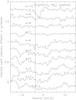 |
Fig. 7 CH3CN(37k−36k) spectra extracted toward the submm continuum position #2 from all k-components. The approximate vlsr is marked by a vertical line, and the spectra are shifted in the y-axis for clarity. |
3.3. Dense gas spectral line emission
As shown in Fig. 2, the region is a typical hot molecular core with extremely rich spectral line emission. In this paper, we focus on the dense gas and dust emission. Therefore, in the following, we concentrate on the hot core and dense molecular gas tracer methyl cyanide which is observed here in its main isotopologue CH3CN and its rarer isotopologue CH CN in the transitions (37k−36k) with k-levels from 0 to 10. CH3CN traces the dense gas and is a well-known tool used to study the dynamics at the center of high-mass star-forming regions (e.g., Cesaroni et al. 2007). Furthermore, the lines of the rotational k-ladder can be used as a thermometer (e.g., Loren & Mundy 1984). Table 2 presents the frequencies and lower level energies El/k of the respective transitions.
Parameters of main CH3CN(37k−36k) lines in spectral window 1 (spw1).
The El/k values between 588 and 1300 K show that we are tracing a very warm gas component. Furthermore, it is interesting to note that we see pure emission only toward the extended parts of submm source #1, whereas toward the regions of peak emission of the central two submm peaks #1 and #2 the spectra are dominated by absorption (Figs. 5–7). In comparison to Fig. 2, where the spectra toward the region of the main peak #1 are shown after averaging over 0.3′′ diameter to show the general absorption and emission features, Fig. 5 presents the corresponding spectra in spw1 toward the regions of all four continuum peaks with a smaller averaging diameter of 0.06′′ (units Jy beam-1). The secondary source #2 is clearly an absorbing source, while source #3 shows weak emission and source #4 mainly exhibits a noise spectrum.
3.3.1. Kinematics of source #1
The absorption spectra toward the main source #1 in Fig. 6 are dominated by blue-shifted absorption (the blended k = 0,1 components are too broad to isolate blue- and red-shifted absorption properly). Hence, the dense gas along the line of sight of that main peak appears to be dominated by outflowing gas kinematics. Interestingly, the CH3CN(3710−3610) component toward the main submm peak #1 exhibits neither absorption nor emission but only a flat noise spectrum. Since this k = 10 component shows clear emission in the immediate environment (see below and Fig. 8), sensitivity seems unlikely to be the reason for that non-detection. The more reasonable explanation is high optical depth of the continuum. With an excitation temperature El/k = 1300 K, the main excitation region of the k = 10 component may stem from inside the τ = 1 surface of the 438 μm continuum emission and can thus be veiled by the continuum.
A different way to analyze the CH3CN data is via spatially imaging the data and discussing the kinematics via moment and position-velocity analysis. Figure 8 presents the first moment maps (intensity-weighted peak velocities) of the CH3CN(37k−36k) data for the k-components 2−10. (k = 0,1 are blended). The figure also shows for comparison the integrated emission of the k = 2 component. This integrated intensity map exhibits a ring-like structure around the main peak with an approximate diameter of ~ 0.28′′, which does not imply a ring-like CH3CN distribution, but it is certainly caused by absorption toward the center. Although this ring-like structure is not entirely smooth, intensity variations within that structure usually do not exceed 3σ. Hence, we refrain from further interpretation of such CH3CN fluctuations.
 |
Fig. 8 CH3CN(37k−36k) first moment maps of the the k-levels 2 to 10 toward the central sources #1 and #2. The top left panel shows the corresponding integrated zeroth moment map of the CH3CN(372−362) transition (integrated from − 13 to +10 km s-1). The white contour outlines the 3σ level of 0.51 Jy km s-1. The other panels all show intensity-weighted velocity maps, and wedges are shown above the k = 2 panels. While the k = 0 map was prepared without any clipping, the first moment maps are clipped at a 4σ level. The black contours present the 438 μm continuum emission in 4σ steps (1σ = 7 mJy beam-1). The synthesized beams are shown for all panels, and a scale-bar (at 2.2 kpc) is presented in the bottom right panel. The diagonal line in the top middle panel of CH3CN(373−263) marks the axis for the position-velocity diagrams shown in Fig. 9. |
 |
Fig. 9 Position-velocity diagrams for the nine CH3CN(37k−36k) transitions toward source #1 along the axis marked in the top middle panel of Fig. 8. The vertical line shows the approximate velocity of rest and the two solid curves present a Keplerian rotation curve for a 10(4.5) M⊙ star at a distance of 2.2(1) kpc. The dashed curves correspond to masses of 5(2.3) and 20(9) M⊙ (inner and outer curves, respectively) at 2.2(1) kpc. |
As shown in Sect. 3.2, the CO(6–5) data reveal a clear outflow in the north-northwest direction and additional high-velocity gas almost perpendicular to this outflow. Based on the main outflow structure and also indicated by the first moment maps, we identify the axis for the rotational structure perpendicular to the main outflow and mark that axis in the CH3CN(373−263) panel in Fig. 8. While this axis is clearly perpendicular to the outflow presented in Sect. 3.2 and Fig. 4, Leurini et al. (2011a) showed multiple outflows emanating from this region. Hence, the CH3CN velocity structure is likely also influenced by additional outflow kinematics. Along this axis marked in Fig. 8 we present position-velocity (pv) cuts for the k = 2...10 components of CH3CN(37k−36k) in Fig. 9. These pv cuts exhibit several interesting features. First, we can clearly identify the absorption structure toward the continuum peak dominated by blue-shifted absorption, again reinforcing that we do not just see the dense rotating structure in the CH3CN gas, but also contributions from the outflow. Furthermore, the pv diagrams partly show structures reminiscent of Keplerian rotation with the highest velocities close to the center and lower velocities farther away from the center. To illustrate this, the pv diagram also shows the expected signature for a Keplerian disk around a 10(4.5) M⊙ star at 2.2(1) kpc. In particular for the k = 2...6 components, the pv diagram reflects this structure. However, there is a caveat to this interpretation. A real Keplerian pv diagram would only show the Keplerian structures as indicated by the lines in Fig. 9, but we see similar structures in the two opposing quadrants of these pv diagrams which are not typical for Keplerian disks. However, Seifried et al. (2016) have recently shown that, depending on the inclination, emission from disks can also appear in these other quadrants of the pv diagrams. Nevertheless, it appears likely that the CH3CN emission includes additional gas components that are not represented by a pure Keplerian rotation model, e.g., emission from the infalling envelope and the outflows (see Sect. 4.2 for further discussion).
3.3.2. Infall motions toward source #2
In contrast to the main peak, the absorption spectra for the secondary peak #2 (see Fig. 7) exhibit absorption on the blue- and red-shifted side of the spectrum. This can be seen in particular for the k-components 2 to 6 (again the 0, 1 components are blended), while the k-components 7 to 9 are showing mainly noise. Interestingly, the k = 10 component of CH3CN in Fig. 7 again shows a clear and pronounced red-shifted absorption feature. However, since the k-7 to 9 components do not show this behavior, we caution that this absorption feature near the k = 10 component may be a line-blend from an unidentified species. Nevertheless, based on the k = 2−6 CH3CN(37k−36k) lines, infall and outflow motion toward/from submm source #2 appears the most likely kinematic interpretation of the data.
We cannot spatially resolve any kinematics, but just analyze the kinematics along the line of sight. In addition to the blue-shifted absorption likely stemming from outflowing gas, the red-shifted absorption spectra in the k = 2...6 components are indicative of infall motions toward that core. If we assume spherical symmetry, we can estimate the mass infall rate with Ṁin = 4πr2ρvin, where Ṁin and vin are the infall rate and infall velocity, and r and ρ the core radius and density (see also Qiu et al. 2011; Beuther et al. 2013). Since the infall rate scales linearly with the distance, the following estimate is only conducted for the distance of 2.2 kpc and can be scaled to 1.0 kpc. We estimate the radius to r ~ 80 AU which is half our spatial resolution limit in the line emission of 0.07′′. For the density estimate, we use ρ ~ 2.3 × 109 cm-3 assuming that the peak column density (Table 1) is smoothly distributed along the line of sight at our spatial-resolution limit (i.e., 160 AU at 2.2 kpc). The infall velocity can be estimated to ~7.1 km s-1, corresponding to the difference between the most red-shifted absorption at ~+ 3.5 km s-1, and the vlsr ~ −3.6 km s-1. Using these physical parameters, we can estimate approximate mass infall rates toward submm source #2 of Ṁin ~ 1.6 × 10⁻³ M⊙ yr-1. At a distance of 1 kpc, that infall rate is a factor of 2.2 lower.
Since collapse motions in star formation are typically associated with outflow and rotational dynamics, we hypothesize a 2D disk-like geometry to refine the infall rate estimate following Beuther et al. (2013). If the accretion follows along a flattened disk-like structure with a solid angle Ω (instead of the 4π in the spherical case), the corresponding disk infall rate Ṁdisk,in scales approximately as  . Following Kuiper et al. (2012, 2015, 2016), an outflow approximately covers an opening angle of 120°, while the disk covers ~60° (both to be doubled to take into account the north-south symmetry). Because opening angles do not scale linearly with the surface elements, full integration results in approximately 50% or ~ 2π being covered by the disk-like structure. Taking these arguments into account, we estimate approximate disk infall rates around Ṁdisk,in ~ 0.8 × 10⁻³ M⊙ yr-1 at a 2.2 kpc distance, or again a factor of 2.2 lower at 1.0 kpc. Although strictly speaking these are disk infall rates and not accretion rates, they can be used as upper limit for the mean actual accretion rates (due to variable accretion from disk to star, the actual accretion rate can be much higher than the large-scale infall rate on short timescales), and they are fully consistent with expected accretion rates for high-mass star formation (e.g., Krumholz et al. 2007b; Beuther et al. 2007a; Zinnecker & Yorke 2007; McKee & Ostriker 2007; Kuiper et al. 2010; Tan et al. 2014).
3.4. Temperature structure
The CH3CN(37k−36k)k-ladder allows a detailed derivation of the gas temperature of the central rotating core/disk structure associated with source #1. With energy levels between 588 and 1300 K (Table 2) we are tracing the hot component of the gas. Since the same spectral setup also covers the CHCN(37k−36k) isotopologue (Fig. 2 and Table 2), high optical depth can also be taken into account. In addition, at the given very high spatial resolution, we do not get just an average temperature, but we can derive the temperature structure pixel by pixel over the full extent of the CH3CN emission. Figure 10 (top panel) shows the integrated zeroth moment map of the CH3CN(372−362) to outline the extent of the CH3CN emission in comparison to the submm continuum.
 |
Fig. 10 Top panel: for source #1 the zeroth moment map for CH3CN(372−362) integrated from –13 to +10 km s-1. The white contour outlines the 3σ level of 0.51 Jy km s-1. Middle panel: rotational temperature map derived with XCLASS from the full CH3CN(37k−36k) ladder (k = 0...10). Temperatures outside the CH3CN(372−362) 3σ level are blanked. Bottom panel: for comparison, the 438 μm continuum emission converted to Planck brightness temperatures. The black contours show in all panels the 438 μm continuum emission in 4σ steps of 28 mJy beam-1. The beam is shown at the bottom right of each panel. |
For the pixel-by-pixel fitting of the CH3CN(37k−36k) data we used the eXtended CASA Line Analysis Software Suite (XCLASS) tool implemented in CASA (Möller et al. 2017). This tool models the data by solving the radiative transfer equation for an isothermal homogeneous object in local thermodynamic equilibrium (LTE) in one dimension, relying on the molecular databases VAMDC and CDMS1. It furthermore uses the model optimizer package Modeling and Analysis Generic Interface for eXternal numerical codes (MAGIX), which helps to find the best description of the data using a certain model (Möller et al. 2013). To fit our data we used the XCLASS version 1.2.0 with CASA version 4.6.
 |
Fig. 11 Example CH3CN(37k−36k) spectrum and corresponding XCLASS two-component fit toward an arbitrary position of CH3CN emission in the disk-like structure around source #1. The corresponding temperature is marked at the top right. |
To fit the data, we explored a broad parameter space and also investigated whether single-component or double-component modeling was more appropriate. The source structure with a central luminous source implies that the temperature structure is more complicated, with temperature gradients, and even shocks may contribute to the gas temperature structure. However, increasing the fit complexity did not improve the fit quality significantly. Temperature results for the central area of interest varied by less than 10% between the single- and double-component fits. Nevertheless, to account at least partly for the complexity, we resorted to a two-component fit. Figure 11 shows one example spectrum and the corresponding XCLASS fit. While this fit itself does not appear great at first look, the differences can be largely attributed to additional spectral lines from other molecular species within the same spectral area.
In the following, we continue our analysis with the warmer of the two components because it resembles the innermost region best. Figure 10 (middle panel) presents the derived hot component temperature map for our central core/disk rotating structure. The hole in the center of the map is caused by the absorption against the strong continuum where no reasonable CH3CN fits are possible. We find very warm gas with temperatures largely around 1000 K with no steep gradient.
For comparison, in the bottom panel of Fig. 10 we also show the 438 μm continuum map, this time converted to Planck brightness temperatures Tb. Since we see all spectral lines in absorption against the main peak, the central position may be optically thick and thus could give an estimate of the dust temperature. The highest value we find this way is 201 K, significantly below the gas temperatures estimated from the CH3CN data. With the unknown exact optical depth, this dust temperature should be considered a lower limit to the actual dust temperature. Since the optical depth decreases going farther out, this assumption breaks down soon after leaving the main peak position. This can also be tested by fitting profiles to the dust continuum map. We explored this by fitting brightness temperatures to the west and east from the center ( ), and we derived profile values α of − 1.7 and − 1.6, respectively. This is far too steep for any reasonable disk or core profile (usually α ~ −0.4; e.g., Kenyon & Hartmann 1987) and hence shows that the dust continuum map cannot be optically thick away from the central position.
4. Discussion
4.1. Fragmentation
The number of submm continuum sources found toward G351.77-0.54 in Fig. 3 appears to be low within that field of view. However, quantifying this more closely, we find four sources (#1 to #4) within a projected separation between #3 and #4 of ~ 7′′, corresponding to 15 400(7000) AU at proposed distances of 2.2(1.0) kpc. Since the continuum optical depth is very high (see Sect. 3.1), the extended structure of source #1 may hide potential additional substructure. Independent of this, the overall continuum structure resembles a proto-Trapezium-like system (e.g., Ambartsumian 1955; Preibisch et al. 1999). Assuming a spherical distribution, this corresponds to source densities of ~ 1.8 × 10⁴ pc-3(2.0 × 10⁵ pc-3) at 2.2(1) kpc distance. These densities are comparable to or are even higher than source densities found in typical embedded clusters (protostellar densities typically around 104 pc-3, Lada & Lada 2003). The separations also compare well to the Orion Trapezium system (e.g., Muench et al. 2008). Furthermore, similar high densities have also been found in a few other high-mass star-forming regions, e.g., W3IRS5 (Rodón et al. 2008) and G29.96 (Beuther et al. 2007c). Although our mass sensitivity is very low ≤0.004 M⊙, the comparably high column density sensitivity of 5 × 1023 cm-2 (Sect. 3.1) indicates that some lower column density sources may be hidden below our sensitivity estimates. Therefore, the above estimated source densities should be considered as lower limits to the actual densities in the region.
4.2. (Disk) rotation?
As described in Sect. 3.3 and shown in Figs. 8 and 9 we identify clear velocity gradients perpendicular to the main CO(6–5) outflow emanating from source #1. However, the position-velocity diagram also shows non-Keplerian contributions in the two opposing quadrants of the pv diagrams in Fig. 9. While inclination effects can partly account for this (e.g., Seifried et al. 2016), models of embedded disks within infalling and rotating structures naturally result in such pv diagrams (e.g., Ohashi et al. 1997; Sakai et al. 2016; Oya et al. 2016).
While ideally one would like to estimate the mass of the central object by fitting a Keplerian curve to the outer structure in the pv diagram (Fig. 9), this seems hardly feasible for G351.77. In comparison to the fiducial 10(4.5) M⊙ Keplerian curve at 2.2(1.0) kpc presented in Fig. 9, we also show the corresponding Keplerian curves for half and double the central masses. Although one could argue that for example the k = 8,9 transitions may be best represented by the 10(4.5) M⊙ curve, this is less obvious in some of the other transitions (e.g., k = 5,6). Unfortunately, this means that determining the exact mass of the central object remains difficult.
Leurini et al. (2011a) note that there also seems to be CH3CN emission associated with the outflow, and if this is the case the interpretation becomes more complicated. We confirm this result in that we see blue-shifted absorption along the line of sight as well as a smaller scale red-shifted CO(6–5) emission feature in the east-northeastern direction (Fig. 4). It is interesting to note that this is the case even for spectral lines with high excitation temperatures (Table 2). Furthermore, outflows can also produce emission features in the other quadrants of the pv diagrams (e.g., Arce et al. 2007; Li et al. 2013).
Hence, although we find a clear velocity gradient perpendicular to an outflow that likely stems – to a significant fraction – from an embedded disk-like structure, there are several additional kinematic signatures attributable to an infalling envelope, as well as outflow emission that complicate the overall interpretation.
4.3. Gas and dust temperatures
Why does the gas temperature derived from the CH3CN(37k−36k)k-ladder deviate so much from the brightness temperature based on the dust continuum emission? To first order, at the high densities present in this region, we expect that gas and dust should be well coupled. For CH3CN, Feng et al. (2015) have shown that not considering optical depth effects may cause significant overestimates of estimated temperatures. However, since XCLASS also takes into account the CHCN(37k−36k) isotopologue emission, this does not seem to be the case here. Therefore, the data indicate that the CH3CN and dust continuum emission may trace different physical entities within the region. While shocks can be partially responsible for differences in the temperature structure, the gas and dust may also trace different components of the expected underlying massive disk. Considering that both emission structures are dominated by a disk-like structure around the central object and are less affected by the envelope because it is filtered out by the extended array used here, the dust continuum emission may trace a colder disk mid-plane, whereas the CH3CN emission may stem more from the disk surface. While this scenario has been discussed for low-mass disks (e.g., Henning & Semenov 2013; Dutrey et al. 2014), it is less well constrained for disks around higher mass young stellar objects. However, from a physical point of view, we expect a similar behavior. Investigating the best-fit model of the high-mass disk source AFGL4176 by Johnston et al. (2015) in more detail, such a temperature structure is found qualitatively as well. We may now see the first observational evidence of that here in G351.77-0.54. In addition to this, since the CH3CN emission may be partly influenced by the outflow, associated shocks may also contribute to the high temperatures.
4.4. Toomre stability of rotating structure
Using the temperature information derived from the CH3CN data, we can also address the stability of the central rotating structure around the main source #1. Originally derived by Toomre (1964) to estimate the gravitational stability of a disk of stars, it has been used since then in various environments for a stability analysis (e.g., Binney & Tremaine 2008). In this framework, the Toomre Q parameter refers to the stability of a differentially rotating, gaseous disk where gravity acts against gas pressure and differential rotation. The Toomre Q parameter is defined as  with the sound speed cs; the epicyclic frequency κ, which corresponds to the rotational velocity Ω in the case of a Keplerian disk; and the surface density Σ. For thin disks, axisymmetric instabilities can occur for Q< 1. Broadening the framework to disks with finite scale-height, the disks can stay stable to slightly lower values because the thickness reduces the gravity in the midplane where typically the structure formation takes place. Studies with different disk density profiles found critical Q values below which axisymmetric instabilities occur between ~0.6 and ~0.7 (e.g., Kim & Ostriker 2007; Behrendt et al. 2015). In contrast to this, non-axisymmetric instabilities like spirals or bars can also occur at slightly higher Q with Q< 2 (e.g., Binney & Tremaine 2008). Taking these differences into account, for Q significantly higher than 2 the disks should stay stable, whereas at lower Q non-axisymmetric and axisymmetric instabilities can occur.
In the following, we estimate the Toomre Q parameter for the whole rotating structure around the main source #1 calculating the sound speed  with the temperature T (Fig. 10) and the mass of the hydrogen nucleus mH, and using the Keplerian velocity Ω around a 10 M⊙ star. The assumption of Keplerian motion appears reasonable for the inner disk considering the position-velocity diagram shown in Fig. 9, and it may become invalid in the outer regions when the disk mass becomes comparable to the mass of the central object and gravitational instabilities can occur. Furthermore, we use our 438 μm continuum map to estimate the column density NH2 (or Σ) at each pixel with the assumptions outlined in Sect. 3.1.
Regarding the temperature for the sound speed and the column density map, we present three different approaches: first, we use the CH3CN derived rotation temperature (Fig. 10) as a temperature proxy. Second, we use a uniform lower temperature of 200 K as temperature proxy that may resemble the dust temperature better (Sects. 3.1 and 4.3). And third, we use a dust temperature distribution with an approximate dust sublimation temperature of 1400 K at 10 AU and then a temperature distribution with radius r as T ∝ r− α. While α = 0.5 corresponds to the classical disk solution (e.g., Kenyon & Hartmann 1987), embedded disks can have lower α values (e.g., the best-fit disk temperature profile for AFGL4176 has α ~ 0.4, Johnston et al. 2015; Johnston et al., in prep.), thus we assume a value of α = 0.4 for our analysis. Figure 12 presents the corresponding Toomre Q maps in the three panels, with the third panel showing Q for T ∝ r-0.4. Since the temperature difference between these approaches is large (>1000 K and below 100 K in the outskirts), we can consider these Toomre Q maps as the bracketing values for the real physical Toomre Q values in this region.
 |
Fig. 12 Color-scales showing in all three panels the Toomre Q map (see text for details) of the disk seen toward source #1. While the top panel uses the rotational temperature derived from CH3CN (Fig. 10) at each pixel to determine the sound speed and column density, the middle panel uses a uniform lower temperature of 200 K for these estimates. The lower panel uses a dust temperature distribution of T ∝ r-0.4 for the calculations (see Sect. 4.3). The black contours show in each panel the 438 μm continuum emission in 4σ steps of 28 mJy beam-1. Toomre Q values outside the CH3CN(372−362) 3σ level (Fig. 10) are clipped out. The beam is shown at the bottom right of each panel. |
There is a large difference between the maps: the Q values are largely >100 for T = Trot, between 5 and 20 for T = 200 K, and between ~ 1.5 and several 100 for the temperature distribution that varies as function of radius. However, even the lowest values in the map derived with the temperature distribution are greater than ~1.5, hence in the axisymmetric stable regime. We note that with a steeper temperature distribution of α = 0.5 the bluish parts in the bottom panel of Fig. 12 would shift below Toomre Q values of 1, but we consider such a steep distribution unlikely considering the deeply embedded phase and the very high gas temperatures measured in CH3CN. Therefore, while we do see subsources and fragments on larger scales (sources #2 to #4), the central disk-like structure around the main source #1 with an approximate diameter of 1000(500) AU at 2.2(1) kpc appears stable against axisymmetric gravitational fragmentation. The main reason for this is the high average temperature of the rotating structure. This should at least be true for the resolved spatial scales. In addition, for Q values between 1 and 2, disks can be prone to asymmetric instabilities such as spiral arms. Hence, it may still be possible that even higher densities exist locally, which then may allow fragmentation on these smaller local scales.
5. Conclusions
The Atacama Large Millimeter Array (ALMA) in band 9 (around 690 GHz) opens an entirely new window for the study of star formation and in particular the formation of the highest mass stars. With correspondingly long baselines we reach unprecedented spatial resolution of ~0.06′′, allowing us to dissect the small-scale structure in high-mass star-forming regions. Here we present the first such study targeting the high-mass star-forming region G351.77-0.54. With a linear resolution of 130(60) AU, we resolve the fragmentation of the dense inner core in the 438 μm continuum emission, as well as the kinematics and temperature structure of the dense gas.
We resolve four submm continuum sources in the field of view which result in approximate protostellar densities between 104 and 105 pc-3 depending on the assumed distance of the source. This should be considered as a lower limit since our column density sensitivity is higher and we may miss lower column density sources in the field. These high protostellar densities are comparable to those found in other proto-Trapezia systems (e.g., Preibisch et al. 1999; Rodón et al. 2008).
The four spectral windows cover a multitude of spectral lines, here we concentrate on the CH3CN(37k−36k)k-ladder that covers excitation levels above ground between 588 and 1300 K, tracing the warmest gas components in the region. Furthermore, we use the CO(6–5) line wing emission to identify high-velocity gas emanating from the main submm continuum source #1 in the north-northwestern direction. The kinematic analysis of the CH3CN data identifies a velocity gradient perpendicular to that outflow. While the position-velocity gradients show hints of Keplerian rotation, there is also an additional component that likely stems from the infalling envelope as well as possible outflow contributions.
The continuum emission at these wavelengths is so strong – with likely high optical depth toward the peak positions – that we identify absorption in the dense gas tracer CH3CN against the continuum sources #1 and #2. While the absorption toward the main source #1 is mainly blue-shifted and hence dominated by outflow motions, toward the secondary unresolved source #2 blue- and red-shifted absorption is identified. These absorption features indicate high rates of mass infall on the order of 10-4 to 10-3 M⊙ yr-1, which can be considered as upper limit proxies for the actual mean accretion rates onto the central source embedded in #2.
Fitting simultaneously the CH3CN(37k−36k) and CHCN isotopologue k-ladders with XCLASS, we derive a rotational temperature map for the main source #1. Very high gas temperatures are found, often in excess of 1000 K. This means that we are apparently seeing part of the hottest molecular component observed to date in dense high-mass star-forming regions. This is reasonable considering the high excitation levels of the used lines. Assuming that at least the central beam of the submm continuum emission is optically thick, we can use its brightness temperature as a proxy of the dust temperature. The highest continuum brightness temperature we find is 201 K, indicating that we see a difference in gas and dust temperature. We may witness here the difference between the colder dust mid-plane and the hotter gaseous surface layer of a high-mass accretion disk, similar to cases known for their low-mass counterparts.
Analyzing the stability of the rotating structure via the Toomre Q parameter, we find that the central disk-like structure always exhibits high Q values, hence it is on the resolvable scales in the axisymmetrically stable regime. However, asymmetric instabilities like spiral arms may still occur on even smaller, as yet unresolved spatial scales.
Acknowledgments
This paper makes use of the following ALMA data: ADS/JAO.ALMA#2013.1.00260.S. ALMA is a partnership of ESO (representing its member states), NSF (USA) and NINS (Japan), together with NRC (Canada) and NSC and ASIAA (Taiwan) and KASI (Republic of Korea), in cooperation with the Republic of Chile. The Joint ALMA Observatory is operated by ESO, AUI/NRAO and NAOJ. We would like to thank Alvaro Sanchez-Monge and Thomas Möller for their continuous help with and improvements on the spectral line fitting program XCLASS. Furthermore, we thank the referee for a detailed report that improved the clarity of the paper. H.B. acknowledges support from the European Research Council under the Horizon 2020 Framework Program via the ERC Consolidator Grant CSF-648505. R.K. acknowledges support from the German Research Foundation under the Emmy Noether Program via the grant No. KU 2849/3-1.
References
- Ambartsumian, V. A. 1955, The Observatory, 75, 72 [NASA ADS] [Google Scholar]
- Arce, H. G., Shepherd, D., Gueth, F., et al. 2007, in Protostars and Planets V, eds. B. Reipurth, D. Jewitt, & K. Keil, 245 [Google Scholar]
- Behrendt, M., Burkert, A., & Schartmann, M. 2015, MNRAS, 448, 1007 [NASA ADS] [CrossRef] [Google Scholar]
- Beltrán, M. T., & de Wit, W. J. 2016, A&ARv, 24, 6 [NASA ADS] [CrossRef] [Google Scholar]
- Beltrán, M. T., Cesaroni, R., Neri, R., & Codella, C. 2011, A&A, 525, A151 [NASA ADS] [CrossRef] [EDP Sciences] [Google Scholar]
- Beuther, H., Schilke, P., Gueth, F., et al. 2002, A&A, 387, 931 [NASA ADS] [CrossRef] [EDP Sciences] [Google Scholar]
- Beuther, H., Zhang, Q., Reid, M. J., et al. 2006, ApJ, 636, 323 [NASA ADS] [CrossRef] [Google Scholar]
- Beuther, H., Churchwell, E. B., McKee, C. F., & Tan, J. C. 2007a, in Protostars and Planets V, eds. B. Reipurth, D. Jewitt, & K. Keil, 165 [Google Scholar]
- Beuther, H., Leurini, S., Schilke, P., et al. 2007b, A&A, 466, 1065 [NASA ADS] [CrossRef] [EDP Sciences] [Google Scholar]
- Beuther, H., Zhang, Q., Bergin, E. A., et al. 2007c, A&A, 468, 1045 [NASA ADS] [CrossRef] [EDP Sciences] [Google Scholar]
- Beuther, H., Walsh, A. J., & Longmore, S. N. 2009, ApJS, 184, 366 [NASA ADS] [CrossRef] [Google Scholar]
- Beuther, H., Linz, H., & Henning, T. 2013, A&A, 558, A81 [NASA ADS] [CrossRef] [EDP Sciences] [Google Scholar]
- Bik, A., Kaper, L., & Waters, L. B. F. M. 2006, A&A, 455, 561 [NASA ADS] [CrossRef] [EDP Sciences] [Google Scholar]
- Binney, J., & Tremaine, S. 2008, Galactic Dynamics: 2nd edn. (Princeton University Press) [Google Scholar]
- Boley, P. A., Linz, H., van Boekel, R., et al. 2013, A&A, 558, A24 [NASA ADS] [CrossRef] [EDP Sciences] [Google Scholar]
- Boley, P. A., Kraus, S., de Wit, W.-J., et al. 2016, A&A, 586, A78 [NASA ADS] [CrossRef] [EDP Sciences] [Google Scholar]
- Bonnell, I. A., Larson, R. B., & Zinnecker, H. 2007, in Protostars and Planets V, eds. B. Reipurth, D. Jewitt, & K. Keil, 149 [Google Scholar]
- Cesaroni, R., Neri, R., Olmi, L., et al. 2005, A&A, 434, 1039 [NASA ADS] [CrossRef] [EDP Sciences] [Google Scholar]
- Cesaroni, R., Galli, D., Lodato, G., Walmsley, C. M., & Zhang, Q. 2007, in Protostars and Planets V, eds. B. Reipurth, D. Jewitt, & K. Keil, 197 [Google Scholar]
- Draine, B. T. 2011, Physics of the Interstellar and Intergalactic Medium (Princeton Series in Astrophysics) [Google Scholar]
- Dutrey, A., Semenov, D., Chapillon, E., et al. 2014, Protostars and Planets VI, 317 [Google Scholar]
- Feng, S., Beuther, H., Henning, T., et al. 2015, A&A, 581, A71 [NASA ADS] [CrossRef] [EDP Sciences] [Google Scholar]
- Greenhill, L. J., Chandler, C. J., Reid, M. J., et al. 2004, in IAU Symp. 221, eds. M. Burton, R. Jayawardhana, & T. Bourke, 155 [Google Scholar]
- Henning, T., & Semenov, D. 2013, Chem. Rev., 113, 9016 [Google Scholar]
- Hildebrand, R. H. 1983, Quant. J. Roy. Astron. Soc., 24, 267 [Google Scholar]
- Ilee, J. D., Wheelwright, H. E., Oudmaijer, R. D., et al. 2013, MNRAS, 429, 2960 [NASA ADS] [CrossRef] [Google Scholar]
- Johnston, K. G., Robitaille, T. P., Beuther, H., et al. 2015, ApJ, 813, L19 [NASA ADS] [CrossRef] [Google Scholar]
- Kenyon, S. J., & Hartmann, L. 1987, ApJ, 323, 714 [NASA ADS] [CrossRef] [Google Scholar]
- Keto, E., & Zhang, Q. 2010, MNRAS, 406, 102 [NASA ADS] [CrossRef] [Google Scholar]
- Kim, W.-T., & Ostriker, E. C. 2007, ApJ, 660, 1232 [NASA ADS] [CrossRef] [Google Scholar]
- Klassen, M., Pudritz, R., Kuiper, R., Peters, T., & Banerjee, R. 2016, ApJ, 823, 28 [NASA ADS] [CrossRef] [Google Scholar]
- Kraus, S., Hofmann, K., Menten, K. M., et al. 2010, Nature, 466, 339 [NASA ADS] [CrossRef] [MathSciNet] [PubMed] [Google Scholar]
- Krumholz, M. R., McKee, C. F., & Klein, R. I. 2005, ApJ, 618, L33 [NASA ADS] [CrossRef] [Google Scholar]
- Krumholz, M. R., Klein, R. I., & McKee, C. F. 2007a, ApJ, 665, 478 [NASA ADS] [CrossRef] [Google Scholar]
- Krumholz, M. R., Klein, R. I., & McKee, C. F. 2007b, ApJ, 656, 959 [NASA ADS] [CrossRef] [Google Scholar]
- Krumholz, M. R., Klein, R. I., McKee, C. F., Offner, S. S. R., & Cunningham, A. J. 2009, Science, 323, 754 [NASA ADS] [CrossRef] [PubMed] [Google Scholar]
- Kuiper, R., & Yorke, H. W. 2013, ApJ, 772, 61 [NASA ADS] [CrossRef] [Google Scholar]
- Kuiper, R., Klahr, H., Beuther, H., & Henning, T. 2010, ApJ, 722, 1556 [CrossRef] [Google Scholar]
- Kuiper, R., Klahr, H., Beuther, H., & Henning, T. 2011, ApJ, 732, 20 [NASA ADS] [CrossRef] [Google Scholar]
- Kuiper, R., Klahr, H., Beuther, H., & Henning, T. 2012, A&A, 537, A122 [NASA ADS] [CrossRef] [EDP Sciences] [Google Scholar]
- Kuiper, R., Yorke, H. W., & Turner, N. J. 2015, ApJ, 800, 86 [NASA ADS] [CrossRef] [Google Scholar]
- Kuiper, R., Turner, N. J., & Yorke, H. W. 2016, ApJ, 832, 40 [NASA ADS] [CrossRef] [Google Scholar]
- Lada, C. J., & Lada, E. A. 2003, ARA&A, 41, 57 [NASA ADS] [CrossRef] [Google Scholar]
- Leurini, S., Codella, C., Zapata, L. A., et al. 2009, A&A, 507, 1443 [NASA ADS] [CrossRef] [EDP Sciences] [Google Scholar]
- Leurini, S., Codella, C., Zapata, L., et al. 2011a, A&A, 530, A12 [NASA ADS] [CrossRef] [EDP Sciences] [Google Scholar]
- Leurini, S., Pillai, T., Stanke, T., et al. 2011b, A&A, 533, A85 [NASA ADS] [CrossRef] [EDP Sciences] [Google Scholar]
- Leurini, S., Codella, C., Gusdorf, A., et al. 2013, A&A, 554, A35 [NASA ADS] [CrossRef] [EDP Sciences] [Google Scholar]
- Li, G.-X., Qiu, K., Wyrowski, F., & Menten, K. 2013, A&A, 559, A23 [NASA ADS] [CrossRef] [EDP Sciences] [Google Scholar]
- López-Sepulcre, A., Codella, C., Cesaroni, R., Marcelino, N., & Walmsley, C. M. 2009, A&A, 499, 811 [NASA ADS] [CrossRef] [EDP Sciences] [Google Scholar]
- Loren, R. B., & Mundy, L. G. 1984, ApJ, 286, 232 [NASA ADS] [CrossRef] [Google Scholar]
- Matthews, L. D., Greenhill, L. J., Goddi, C., et al. 2010, ApJ, 708, 80 [NASA ADS] [CrossRef] [Google Scholar]
- McKee, C. F., & Ostriker, E. C. 2007, ARA&A, 45, 565 [NASA ADS] [CrossRef] [Google Scholar]
- McKee, C. F., & Tan, J. C. 2003, ApJ, 585, 850 [NASA ADS] [CrossRef] [MathSciNet] [Google Scholar]
- Möller, T., Bernst, I., Panoglou, D., et al. 2013, A&A, 549, A21 [NASA ADS] [CrossRef] [EDP Sciences] [Google Scholar]
- Möller, T., Endres, C., & Schilke, P. 2017, A&A, 598, A7 [NASA ADS] [CrossRef] [EDP Sciences] [Google Scholar]
- Muench, A., Getman, K., Hillenbrand, L., & Preibisch, T. 2008, Star Formation in the Orion Nebula I: Stellar Content, ed. B. Reipurth, 483 [Google Scholar]
- Müller, H. S. P., Thorwirth, S., Roth, D. A., & Winnewisser, G. 2001, A&A, 370, L49 [NASA ADS] [CrossRef] [EDP Sciences] [Google Scholar]
- Norris, R. P., Whiteoak, J. B., Caswell, J. L., Wieringa, M. H., & Gough, R. G. 1993, ApJ, 412, 222 [NASA ADS] [CrossRef] [Google Scholar]
- Ohashi, N., Hayashi, M., Ho, P. T. P., & Momose, M. 1997, ApJ, 475, 211 [Google Scholar]
- Ossenkopf, V., & Henning, T. 1994, A&A, 291, 943 [NASA ADS] [Google Scholar]
- Oya, Y., Sakai, N., López-Sepulcre, A., et al. 2016, ApJ, 824, 88 [NASA ADS] [CrossRef] [Google Scholar]
- Preibisch, T., Balega, Y., Hofmann, K.-H., Weigelt, G., & Zinnecker, H. 1999, New Astron., 4, 531 [NASA ADS] [CrossRef] [Google Scholar]
- Qiu, K., Zhang, Q., & Menten, K. M. 2011, ApJ, 728, 6 [NASA ADS] [CrossRef] [Google Scholar]
- Rodón, J. A., Beuther, H., Megeath, S. T., & van der Tak, F. F. S. 2008, A&A, 490, 213 [NASA ADS] [CrossRef] [EDP Sciences] [Google Scholar]
- Sakai, N., Oya, Y., López-Sepulcre, A., et al. 2016, ApJ, 820, L34 [NASA ADS] [CrossRef] [Google Scholar]
- Sandell, G., & Wright, M. 2010, ApJ, 715, 919 [NASA ADS] [CrossRef] [Google Scholar]
- Schreyer, K., Henning, T., van der Tak, F. F. S., Boonman, A. M. S., & van Dishoeck, E. F. 2002, A&A, 394, 561 [NASA ADS] [CrossRef] [EDP Sciences] [Google Scholar]
- Schuller, F., Menten, K. M., Contreras, Y., et al. 2009, A&A, 504, 415 [NASA ADS] [CrossRef] [EDP Sciences] [Google Scholar]
- Seifried, D., Banerjee, R., Klessen, R. S., Duffin, D., & Pudritz, R. E. 2011, MNRAS, 417, 1054 [NASA ADS] [CrossRef] [Google Scholar]
- Seifried, D., Sánchez-Monge, Á., Walch, S., & Banerjee, R. 2016, MNRAS, 459, 1892 [Google Scholar]
- Smith, R. J., Longmore, S., & Bonnell, I. 2009, MNRAS, 400, 1775 [NASA ADS] [CrossRef] [Google Scholar]
- Tan, J. C., Beltrán, M. T., Caselli, P., et al. 2014, Protostars and Planets VI, 149 [Google Scholar]
- Tanaka, K. E. I., Tan, J. C., & Zhang, Y. 2016, ApJ, 818, 52 [NASA ADS] [CrossRef] [Google Scholar]
- Toomre, A. 1964, ApJ, 139, 1217 [NASA ADS] [CrossRef] [Google Scholar]
- Walsh, A. J., Burton, M. G., Hyland, A. R., & Robinson, G. 1998, MNRAS, 301, 640 [NASA ADS] [CrossRef] [Google Scholar]
- Wyrowski, F., Güsten, R., Menten, K. M., Wiesemeyer, H., & Klein, B. 2012, A&A, 542, L15 [NASA ADS] [CrossRef] [EDP Sciences] [Google Scholar]
- Yorke, H. W., & Sonnhalter, C. 2002, ApJ, 569, 846 [NASA ADS] [CrossRef] [Google Scholar]
- Zapata, L. A., Leurini, S., Menten, K. M., et al. 2008, AJ, 136, 1455 [NASA ADS] [CrossRef] [Google Scholar]
- Zinnecker, H., & Yorke, H. W. 2007, ARA&A, 45, 481 [NASA ADS] [CrossRef] [Google Scholar]
All Tables
All Figures
|
Fig. 1 uv-plane coverage of these observations toward our target source. |
| In the text | |
|
Fig. 2 Spectra from the four spectral units (spw0 to spw3) extracted toward the main submm peak source #1 (Table 1) and averaging over 0.3′′ diameter. The spectra are ordered by frequency, not spectral window units. The top two panels are the lower sideband and the bottom two panels the upper sideband. A few interesting lines and an almost line-free part in spw0 are also marked. |
| In the text | |
|
Fig. 3 438 μm continuum image of G351.77-0.54. The left panel shows a larger area encompassing the two central sources, as well as two additional submm sources in the southeast and northwest (all marked). The white crosses mark the cm continuum sources by Zapata et al. (2008). The right panel then shows a zoom into the center; the triangles present the class II CH3OH masers from Walsh et al. (1998). The contour levels start at 4σ and continue in 2σ steps with the 1σ level of 7 mJy beam-1. The synthesized beam of 0.06′′ and a scale-bar for an assumed distance of 2.2 kpc are presented as well. |
| In the text | |
|
Fig. 4 438 μm continuum image with CO(6–5) red-shifted emission in red contours. The continuum contours are in 4σ steps (1σ = 7 mJy beam-1). The blue dotted contours show the corresponding negative features. The CO emission was integrated from 25 to 42 km s-1 and is shown in contours from 15 to 95% (step 10%) of the peak emission. The center coordinates are those of the phase center presented in Sect. 2. |
| In the text | |
|
Fig. 5 Spectra extracted toward all four submm peaks in spectral win spw1 averaged over 0.06′′ diameter (units Jy beam-1). |
| In the text | |
|
Fig. 6 CH3CN(37k−36k) spectra extracted toward the submm continuum peak position #1 from all k-components. The approximate vlsr is marked by a vertical line, and the spectra are shifted in the y-axis for clarity. |
| In the text | |
|
Fig. 7 CH3CN(37k−36k) spectra extracted toward the submm continuum position #2 from all k-components. The approximate vlsr is marked by a vertical line, and the spectra are shifted in the y-axis for clarity. |
| In the text | |
|
Fig. 8 CH3CN(37k−36k) first moment maps of the the k-levels 2 to 10 toward the central sources #1 and #2. The top left panel shows the corresponding integrated zeroth moment map of the CH3CN(372−362) transition (integrated from − 13 to +10 km s-1). The white contour outlines the 3σ level of 0.51 Jy km s-1. The other panels all show intensity-weighted velocity maps, and wedges are shown above the k = 2 panels. While the k = 0 map was prepared without any clipping, the first moment maps are clipped at a 4σ level. The black contours present the 438 μm continuum emission in 4σ steps (1σ = 7 mJy beam-1). The synthesized beams are shown for all panels, and a scale-bar (at 2.2 kpc) is presented in the bottom right panel. The diagonal line in the top middle panel of CH3CN(373−263) marks the axis for the position-velocity diagrams shown in Fig. 9. |
| In the text | |
|
Fig. 9 Position-velocity diagrams for the nine CH3CN(37k−36k) transitions toward source #1 along the axis marked in the top middle panel of Fig. 8. The vertical line shows the approximate velocity of rest and the two solid curves present a Keplerian rotation curve for a 10(4.5) M⊙ star at a distance of 2.2(1) kpc. The dashed curves correspond to masses of 5(2.3) and 20(9) M⊙ (inner and outer curves, respectively) at 2.2(1) kpc. |
| In the text | |
|
Fig. 10 Top panel: for source #1 the zeroth moment map for CH3CN(372−362) integrated from –13 to +10 km s-1. The white contour outlines the 3σ level of 0.51 Jy km s-1. Middle panel: rotational temperature map derived with XCLASS from the full CH3CN(37k−36k) ladder (k = 0...10). Temperatures outside the CH3CN(372−362) 3σ level are blanked. Bottom panel: for comparison, the 438 μm continuum emission converted to Planck brightness temperatures. The black contours show in all panels the 438 μm continuum emission in 4σ steps of 28 mJy beam-1. The beam is shown at the bottom right of each panel. |
| In the text | |
|
Fig. 11 Example CH3CN(37k−36k) spectrum and corresponding XCLASS two-component fit toward an arbitrary position of CH3CN emission in the disk-like structure around source #1. The corresponding temperature is marked at the top right. |
| In the text | |
|
Fig. 12 Color-scales showing in all three panels the Toomre Q map (see text for details) of the disk seen toward source #1. While the top panel uses the rotational temperature derived from CH3CN (Fig. 10) at each pixel to determine the sound speed and column density, the middle panel uses a uniform lower temperature of 200 K for these estimates. The lower panel uses a dust temperature distribution of T ∝ r-0.4 for the calculations (see Sect. 4.3). The black contours show in each panel the 438 μm continuum emission in 4σ steps of 28 mJy beam-1. Toomre Q values outside the CH3CN(372−362) 3σ level (Fig. 10) are clipped out. The beam is shown at the bottom right of each panel. |
| In the text | |
Current usage metrics show cumulative count of Article Views (full-text article views including HTML views, PDF and ePub downloads, according to the available data) and Abstracts Views on Vision4Press platform.
Data correspond to usage on the plateform after 2015. The current usage metrics is available 48-96 hours after online publication and is updated daily on week days.
Initial download of the metrics may take a while.