| Issue |
A&A
Volume 603, July 2017
|
|
|---|---|---|
| Article Number | A35 | |
| Number of page(s) | 7 | |
| Section | The Sun | |
| DOI | https://doi.org/10.1051/0004-6361/201629663 | |
| Published online | 04 July 2017 | |
Investigating the behaviour of neutral hydrogen Lyα spectral line width in polar coronal holes at solar minimum
1 INAF–Catania Astrophysical Observatory, 95123 Catania, Italy
e-mail: This email address is being protected from spambots. You need JavaScript enabled to view it.
2 INAF–Turin Astrophysical Observatory, 10025 Pino Torinese (TO), Italy
Received: 7 September 2016
Accepted: 28 March 2017
Abstract
We investigate the behaviour of the H I Lyα spectral line widths measured by UVCS/SOHO in polar coronal holes at minimum of solar magnetic activity. The line widths are reported to significantly increase up to 3 R⊙, while above 3 R⊙ there is observational evidence of either nearly constant or slightly decreasing values. We adopt empirical models of polar coronal holes at solar activity minimum reported in the literature and calculate the characteristic timescales relevant to different processes coupling neutral hydrogen atoms and protons, which are heated and accelerated in the outflowing plasma. This analysis leads us to believe that the progressive decoupling of the two sets of particles below 10 R⊙, caused by the decrease of the plasma density due to the rapid expansion of the wind, cannot explain the behaviour of the Lyα line profile observed in polar coronal holes. We also synthesise the intensity and profile of the Lyα line as a function of heliocentric distance from the coronal hole models, adopting H I densities computed in non-equilibrium ionisation with the aim of satisfactorily reproducing the UVCS Lyα observations reported in the literature. Our analysis shows that the coronal Lyα emission decreases with heliocentric distance, down to values below the interplanetary Lyα emission, owing to the decrease of the plasma density and to non-equilibrium ionisation effects in the expanding plasma. This can lead to the predominance of the interplanetary emission, which is characterised by H I velocity distributions corresponding to temperatures about one order of magnitude lower than the coronal temperatures, and to the narrowing of the resulting coronal profile at higher heliocentric distances. This scenario can be a plausible explanation for the behaviour of the Lyα line profile with height observed in polar coronal holes at solar activity minimum.
Key words: Sun: corona / solar wind / Sun: UV radiation
© ESO, 2017
1. Introduction
One of the most remarkable features revealed by spectroscopic observations of polar coronal holes at solar minimum is the steep increase of coronal line widths with height, in particular for heliocentric distances below 3 R⊙ (Antonucci et al. 1997a, 2000a; Kohl et al. 1997; Suleiman et al. 1999; Akinari 2008).
The UltraViolet Coronagraph Spectrometer (UVCS; Kohl et al. 1995) on board the SOlar and Heliospheric Observatory (SOHO; Domingo et al. 1995) has facilitated the estimation of the line width of H I Lyα, which is the most intense UV spectral line observed in the extended corona, and has revealed an increase of the corresponding kinetic temperature from less than 2 MK at 1.5 R⊙ (see e.g. Akinari 2007) to about 3 MK and more at 3 R⊙ (Esser et al. 1999; Antonucci et al. 2000a,b; Akinari 2008). Above 3 R⊙, observations show either nearly constant (Cranmer et al. 1999a; Antonucci et al. 2000a,b) or slightly decreasing with height kinetic temperatures (Antonucci 1999, 2006; Suleiman et al. 1999; Akinari 2008; Susino et al. 2008). Heavier ions such as O VI exhibit spectral line widths increasing up to 100 MK at 3 R⊙ (Cranmer et al. 1999a; Antonucci et al. 2000a,b; Akinari 2008). At higher altitudes, the oxygen kinetic temperature flattens with fluctuations around its maximum value of about 100 MK (Antonucci 2006; Antonucci et al. 2012; Telloni et al. 2007).
The considerably high temperatures found in coronal holes for O VI ions have been explained as the signature of preferential plasma heating and acceleration via the absorption of Alfvén waves at ion cyclotron frequency (Cranmer et al. 1999b; Hu et al. 1999; Telloni et al. 2007). Understanding the trend observed for the H I Lyα line width beyond 3 R⊙ requires further investigation with the prospect of obtaining accurate analyses of UVCS/SOHO observations. This is important because the information obtained from the characteristics of the Lyα line is generally used to infer the physical conditions of protons in the solar corona. The coronal H I Lyα is principally formed through resonant scattering of chromospheric photons by the neutral hydrogen atoms in the extended solar corona, and only in a small fraction by collisionally excited atoms (Withbroe et al. 1982). In the inner corona (i.e. below 3 R⊙), H I atoms and protons are strongly coupled through different processes, such as photo-ionisation, collisional ionisation, radiative recombination, and charge-exchange (Olsen et al. 1994; Allen et al. 1998). Therefore, neutral hydrogen atoms have nearly the same velocity distribution and, in turn, the same kinetic temperature of the protons, which are heated and accelerated in the solar wind.
At higher altitudes, however, H I atoms could progressively decouple from protons owing to the decrease of the plasma density caused by the rapid expansion of the wind, which reduces the rate of collisions between protons and hydrogen atoms. The decrease in density can also give rise to other non-local effects such as non-equilibrium ionisation (see e.g. Ko et al. 1997) because outflowing hydrogen ions can undergo variations of temperature on timescales much shorter than the relevant ionisation and recombination times; so they may remember the previous plasma ionisation and thermal state as they enter a new temperature range. Hence the neutral hydrogen velocity distribution may not fully reflect the local proton velocity distribution. The progressive decoupling of the H I atoms from the fast solar wind protons (Allen et al. 1998, 2000) might be a plausible explanation of the behaviour of the H I Lyα line width beyond 3 R⊙. In addition, the decrease in density also causes a depletion of the coronal Lyα emission, which can become significantly less intense than the corresponding emission of the interplanetary plasma (see e.g. Akinari 2008), which is characterised by H I velocity distributions corresponding to temperatures of the order of 104–105 K (Bertaux et al. 1997; Quémerais et al. 2006). All this might explain the observed narrowing of the H I Lyα profile.
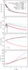 |
Fig. 1 Radial profiles of the coronal hole plasma parameters for the considered models: a) electron density; b) electron temperature; c) parallel (solid lines) and perpendicular (dot-dashed lines) components of the H I kinetic temperature; and d) outflow wind velocity. Electron densities and temperatures from Ko et al. (1997), David et al. (1998), Wilhelm et al. (1998), Esser et al. (1999), and Antonucci et al. (2004) are also reported for comparison. |
In order to investigate more quantitatively the role of the effects listed above and evaluate their importance in determining the variations of the neutral hydrogen Lyα line width as a function of the heliocentric distance in polar coronal holes, we calculated the characteristic timescales relevant to the processes responsible for the coupling of protons and neutral atoms in the corona. We used empirical models of polar coronal holes at solar minimum for the plasma parameters (Cranmer et al. 1999a; Guhathakurta et al. 1999). We also synthesised the intensity and profile of the Lyα line as a function of the heliocentric distance and compared the results with some available UVCS observations reported by Cranmer et al. (1999a), Suleiman et al. (1999), and Akinari (2008).
2. Characteristic timescales for the coupling of neutral hydrogen atoms and protons
2.1. Models of polar coronal holes
We calculated the characteristic timescales relevant to the processes responsible for the coupling of neutral atoms and protons in the corona (whose definitions are reported in Allen et al. 1998) for three empirical models of the polar coronal hole at solar minimum characterised by different morphology and physical conditions: models A1 and A2 of Cranmer et al. (1999a) and the model of Guhathakurta et al. (1999). We modified model A1 of Cranmer et al. (1999a) iteratively fine-tuning the plasma parameters in the original model to obtain the best fit of the computed to the observed Lyα spectral line profiles (see Sect. 3, for details on the observations). The original electron density radial dependence on the heliocentric distance of model A1 (the same of model A2) was kept unchanged in the iterative process.
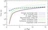 |
Fig. 2 H I mean lifetime (red line) and theoretical timescales computed for charge-exchange (blue line), H I-p coupling (dotted line), recombination (green line), photo-ionisation (light blue line), collisional ionisation (yellow line), and solar wind expansion (dashed line), as functions of the heliocentric distance for our coronal hole model. The H I mean lifetime and the H I-p coupling time curves overlap each other. |
The final radial profiles of the electron density and temperature, parallel and perpendicular components of the H I kinetic temperature (with respect to the magnetic field direction, assumed to be radial in coronal holes), and wind outflow velocity for the modified model A1 (hereafter called our model) and for the other two considered models are reported in Fig. 1. For comparison, we plotted the electron density measurements obtained by Wilhelm et al. (1998) and Antonucci et al. (2004) in polar coronal holes during the minimum of solar activity, as well as the electron temperature measurements obtained by David et al. (1998) in the same coronal hole observed by Antonucci et al. (2004). These values are spectroscopically derived from the ratios of UV emission lines and, although limited to lower heliocentric distances, represent important constraints to the models. The electron density and temperature profiles from Esser et al. (1999) and the electron temperature profile from Ko et al. (1997) are also shown. Panel a reports the electron density versus heliocentric distance for the adopted models together with the electron densities from Wilhelm et al. (1998), Esser et al. (1999), and Antonucci et al. (2004). The radial profile of our model and that of model A2 of Cranmer et al. (1999a) are coincident. The radial profiles of the other authors are significantly lower, particularly below 2 R⊙. Panel b shows the electron temperature versus heliocentric distance for the three models considered and the electron temperatures reported by Ko et al. (1997), David et al. (1998), and Esser et al. (1999). The temperature profile of our model exhibits a behaviour similar to those of the models A2 of Cranmer et al. (1999a), Ko et al. (1997), and Esser et al. (1999), but our profile is about a factor of two lower. It is even lower (about a factor of four) than the radial profile of Guhathakurta et al. (1999). Below 1.5 R⊙, it is consistent with the measurements of David et al. (1998). Panel c reports the parallel and perpendicular components of the H I kinetic temperature. In our model and in that of Guhathakurta et al. (1999) the parallel component was assumed to be equal to the electron temperature. The radial profile of the parallel component of the H I kinetic temperature for model A2 of Cranmer et al. (1999a) is missing because the model is isotropic. The temperature of the perpendicular component for Guhathakurta et al. (1999) has been assumed to be equal to that of our model. Finally, panel d shows the outflow wind velocity versus heliocentric distance for the three considered models. Model A2 of Cranmer et al. (1999a) shows the highest outflow wind velocities (a factor of about 1.6 higher than the others), while the wind velocities of Guhathakurta et al. (1999) are nearly coincident with those of our model above 2 R⊙.
2.2. Comparison among characteristic timescales
The theoretical timescales for collisional ionisation, photo-ionisation, recombination, and charge-exchange, as well as the H I mean lifetime, solar wind expansion time, and H I-p coupling time, computed for the plasma parameters of our coronal hole model are all reported in Fig. 2 as functions of the heliocentric distance. The radial behaviour of the characteristic timescales for the other two adopted models is similar. It is worth noting that the recombination timescale is always much higher than all the other timescales, and, in particular, than the solar wind expansion time, which, in turn, becomes comparable to those of collisional ionisation and photo-ionisation processes already at 4–5 R⊙. All this could give rise to significant departures from ionisation equilibrium. In order to evaluate these departures, we calculated proton and neutral hydrogen densities in the coronal hole as a function of heliocentric distance for all the considered models, in both ionisation equilibrium and non-equilibrium conditions, using the numerical code for the solution of the ionisation balance equations reported in Spadaro & Ventura (1994). In the case of our coronal hole model, the non-equilibrium neutral hydrogen density is lower than the equilibrium one by a factor of about two above 3 R⊙, as shown in Fig. 3. A similar result is obtained for the other coronal hole models.
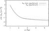 |
Fig. 3 Non-equilibrium (solid line) and equilibrium (dashed line) H I density vs. heliocentric distance for our coronal hole model. |
Conversely, the charge-exchange timescale, which is close to the H I-p coupling time at all altitudes, becomes comparable to the wind expansion time only beyond about 10 R⊙ (see e.g. Allen et al. 1998); this is well outside the heliocentric distance range considered in this study and for which UVCS observations are typically reported. Hence the rate of the charge-exchange processes between the H I atoms and protons is higher than the solar wind expansion rate, such that the decoupling is negligible below 10 R⊙ and does not significantly affect the behaviour of the Lyα line profile in polar coronal holes. Note that this is the criterion for decoupling in the direction parallel to the magnetic field, as discussed by Allen et al. (1998). The results of their model, describing plasma conditions typical of the fast solar wind, indicate that significant decoupling in the direction perpendicular to the magnetic field already occurs at altitudes of 3 R⊙ for reasonable high-speed solutions in which the interaction rate between the protons and neutral hydrogen atoms is much smaller than the frequency of the Alfvén waves propagating in the corona parallel to the magnetic field lines and directly affecting the radially outflowing protons. For the polar coronal hole models used here, we expect interaction rates well below 0.01 Hz at altitudes of 3 R⊙ and higher, therefore much smaller than the highest frequency (~ 1 Hz) of the Alfvén waves spectrum considered by Allen et al. (1998). As a result, neutral hydrogen atoms and protons should decouple in the direction perpendicular to the magnetic field above 3 R⊙. On the other hand, the calculations of Allen et al. (1998) suggest that the perpendicular component of the velocity distribution of hydrogen, which is the dominant contributor to the Lyα line profile for the relevant lines of sight, is increasing and higher than that of protons in the range of heliocentric distances up to 5 R⊙, becoming lower than that of protons only above 10 R⊙ (see also Allen et al. 2000). Hence, this kind of decoupling cannot explain the behaviour of the Lyα line profile observed in polar coronal holes.
3. Synthesis of H I Lyα intensity and profile in coronal holes
We synthesised the intensity and profile of the Lyα line emerging from a polar coronal hole as a function of the heliocentric distance by means of an improved version of the numerical code developed by Ventura & Spadaro (1999). We adopted the empirical models of the polar coronal hole reported in Sect. 2.1 and used neutral hydrogen densities computed without the assumption of equilibrium ionisation. The geometry of the coronal hole models A1 and A2 of Cranmer et al. (1999a), which is the same adopted for our model, and of the model of Guhathakurta et al. (1999) is reported in Fig. 4 as a schematic 2D plot showing the expansion of the coronal hole versus heliocentric distance, where the X axis is parallel to the line of sight (LOS).
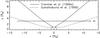 |
Fig. 4 Schematic 2D plot of the geometry of the adopted coronal hole models. The horizontal line represents the line of sight (LOS) at 3 R⊙. |
The spectral synthesis code calculates both the radiatively and collisionally excited components of coronal Lyα, taking into account a bi-Maxwellian velocity distribution of neutral hydrogen atoms and the Doppler dimming effects on the Lyα line caused by the wind outflow (Hyder & Lytes 1970; Noci et al. 1987; Withbroe et al. 1982). The integration of the coronal line emission is performed over the entire coronal hole extent along the LOS (see Spadaro et al. 2007; Ventura & Spadaro 1999) in the direction shown in Fig. 4. We also took into account the contribution of the wind outflow velocity component along the LOS to the Doppler broadening of the line (see e.g. Akinari 2007). The chromospheric Lyα line profile adopted in the Doppler dimming calculations is reported in Fig. 5 (see Dolei et al. 2015).
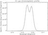 |
Fig. 5 Adopted chromospheric Lyα line profile. Details and analytical form are reported in Dolei et al. (2015). |
We then combined the synthetic Lyα coronal profile with the UVCS stray-light contribution estimated according to Gardner et al. (1996) and the interplanetary Lyα profile observed by UVCS above 6 R⊙ (Kohl et al. 1997; Suleiman et al. 1999; Akinari 2008), which is assumed to be constant over the entire considered heliocentric distance range (see Sect. 4).
Finally, we compared the total Lyα profile versus heliocentric distance with the UVCS line profiles reported in Cranmer et al. (1999a), Suleiman et al. (1999), and Akinari (2008). These works refer to observations of both north and south solar minimum polar coronal holes at projected heliocentric heights from 1.25 to 5 R⊙, spanning the time interval May 1996 – January 1998, between the phase of minimum solar activity at the end of cycle 22 (Cranmer et al. 1999a; Akinari 2008) and the initial rising phase of cycle 23 (Suleiman et al. 1999). The Lyα line intensities and 1/e half width profiles reported by Cranmer et al. (1999a) and Akinari (2008) are averaged over time, putting together observations performed at the same heliocentric distance. The data reported in Suleiman et al. (1999) refer only to the 1/e half widths deduced by Lyα line profile observations performed in a South polar coronal hole from 1.5 to 6 R⊙ and have been taken as they stand. For more information on the observation logs and data reduction, we refer to the detailed descriptions given by Cranmer et al. (1999a), Suleiman et al. (1999), and Akinari (2008). In all the considered cases, observations include a mixed contribution from both plume and inter-plume regions, located along the LOS and over the portion of the UVCS entrance slit spatially binned to improve the count statistics (see Sect. 4, for a discussion on possible effects that these occurrences might have on our results). The observations by Cranmer et al. (1999a) and the other two groups differ significantly, particularly in the line width (see Fig. 6). The data reported by Suleiman et al. (1999), which are relevant to the initial rising phase of cycle 23, are in a better agreement with those of Akinari (2008); however, they are not in agreement with those of Cranmer et al. (1999a) even though the last two data sets refer to the same phase of solar activity. Therefore the different observation times may not fully explain the differences in the reported data. On the other hand, the uncertainties affecting the 1/e half width data of Cranmer et al. (1999a) are much larger than those reported by the other two groups. This could significantly reduce the discrepancy above 3 R⊙.
4. Results and discussion
The radial profiles of the total Lyα intensity (including stray-light and interplanetary contributions) and 1/e half width of the H I velocity distribution, derived from the width of the spectral line profile, are shown as solid bold lines in Fig. 6 for the three models considered here. In each plot, the solid thin line refers to the coronal line profile predicted from the relevant model, the dotted line to the estimated UVCS stray-light component (Gardner et al. 1996), and the dashed line to the assumed interplanetary (IP) Lyα line (Kohl et al. 1997; Suleiman et al. 1999; Akinari 2008).
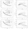 |
Fig. 6 Synthesised Lyα line intensities (left panels) and 1/e half widths of the H I velocity distribution (right panels) vs. heliocentric distance, compared with the values deduced by the observations of several authors. Top panels report the results of our model, middle panels those of the model of Guhathakurta et al. (1999), and bottom panels those of the model A2 of Cranmer et al. (1999a). |
The coronal Lyα line emission predicted by our model is always higher than that of the stray-light component, but it becomes less intense than the interplanetary Lyα line above 4 R⊙ (see top left panel in Fig. 6). This aspect was also noted by Akinari (2008) in his systematic survey of Lyα line profiles observed by UVCS/SOHO in polar coronal holes at solar minimum. The depletion of the coronal Lyα emission is due to the decrease of plasma density at higher altitudes, which is caused by the rapid expansion of the wind. Moreover, an additional depletion occurs in our calculations as a consequence of significant non-equilibrium ionisation effects in the expanding plasma, which leads to lower coronal neutral hydrogen densities (by about a factor of two with respect to the densities calculated under the assumption of equilibrium ionisation). The reduction in the coronal Lyα intensity versus heliocentric distance is steeper for the model of Guhathakurta et al. (1999; see middle left panel in Fig. 6) because of the lower electron density over the entire range of considered heliocentric distances. It is even steeper for the model A2 of Cranmer et al. (1999a) because the significantly higher outflow velocity gives rise to a more effective Doppler dimming of the coronal Lyα emission. This already becomes less intense than the interplanetary Lyα line slightly above 3 R⊙ and even lower than that of the stray-light component above 3.5 R⊙ (see bottom left panel in Fig. 6).
Figure 6 also shows a comparison of the line intensities and profiles calculated for the three models considered here with the observed values reported by Cranmer et al. (1999a), Akinari (2008), and Suleiman et al. (1999). A comparison of the line profiles is only possible with the last authors. Akinari (2008) decomposed the observed Lyα line profiles into two Gaussian components with different widths (a narrow and a super-narrow component, the latter being observable at heights greater than 2.9 R⊙). However, in order to make possible a direct comparison with the total profile computed for the three coronal hole models considered in this work (i.e. including stray-light and interplanetary components), we reconstructed the total profile observed by Akinari (2008) according to the data shown in Figs. 5–7 of the cited paper; in addition, we reported the corresponding intensities and 1/e half widths as diamonds in all the plots. Furthermore, the radial behaviour of the neutral hydrogen kinetic temperature deduced by the Lyα 1/e half widths obtained by Suleiman et al. (1999) and Akinari (2008) agrees very well with that reported in the review of Antonucci (1999); this is relevant to a polar coronal hole observed at minimum of solar activity.
The comparison of the intensities and 1/e half widths of the velocity distribution predicted from our model (solid thin lines in top panels) with the observations reported by Cranmer et al. (1999a) gives a satisfactory agreement. However, a discrepancy is evident when we compare the total intensities and 1/e half widths (solid bold lines in top panels). In particular, the 1/e half widths exhibit a clear decreasing trend above 3 R⊙, while those derived from the Lyα line profiles observed by Cranmer et al. (1999a) show a nearly constant behaviour (see top right panel in Fig. 6). On the other hand, the uncertainties affecting the 1/e half width data reported by Cranmer et al. (1999a) are so large (up to 90 km s-1) that a decreasing trend above 3 R⊙ cannot be ruled out.
Conversely, the total intensities and 1/e half widths of our model (solid bold lines in top panels) agree well with those reported by Suleiman et al. (1999) and Akinari (2008). More specifically, they satisfactorily reproduce the intensities and, to a lesser extent, the line widths observed by Akinari (2008). The 1/e half width values derived by Suleiman et al. (1999) are very well matched by our calculations.
The decrease of the coronal Lyα emission with heliocentric distance down to values below the interplanetary Lyα component, evident in the top left panel of Fig. 6, could then lead to the predominance above a certain height in the corona of the interplanetary emission, which is characterised by H I velocity distributions corresponding to temperatures of the order of 104–105 K (Bertaux et al. 1997; Quémerais et al. 2006). This can give rise to the narrowing of the resulting coronal H I Lyα line profile at higher heliocentric distances and therefore be a plausible explanation for the behaviour of the Lyα line profile above 3 R⊙ observed by Suleiman et al. (1999) and Akinari (2008).
As for the total Lyα line intensities and 1/e half widths obtained for the models of Guhathakurta et al. (1999) and A2 of Cranmer et al. (1999a; solid bold lines in middle and bottom panels, respectively), we note a less satisfactory reproduction of the observed line intensities and widths and that such models were not adjusted to better fit the observations. In particular, the behaviour of the 1/e half width still exhibits the initial increase and a subsequent decrease at higher heliocentric distances, thereby very well reproducing the widths observed by Suleiman et al. (1999) and Akinari (2008) above 4 R⊙. However, the agreement is poorer at lower heliocentric distances. The steeper decrease in the coronal Lyα emission predicted by these models results in the predominance of the interplanetary emission at lower coronal heights with respect to our model, giving significantly narrower line widths than observed between 2 and 4 R⊙. In any case, we can conclude that the synthetic coronal line profiles calculated for the coronal hole models of Guhathakurta et al. (1999) and A2 of Cranmer et al. (1999a) generally confirm the explanation of the behaviour of the Lyα line profile suggested above on the basis of our model.
A discussion is in order of other observational effects and plasma processes that might affect the coronal Lyα line profile and lead to a decrease of line widths at higher heliocentric distances.
For instance, plumes are denser and cooler than the background coronal hole plasma (see e.g. Antonucci et al. 1997b; Antonucci 1999; Giordano et al. 2000). Mixing the two contributions would affect the intensity and shape of the averaged line profiles, as investigated by Raouafi et al. (2007). These authors report the results of a comparison between UVCS observation of polar coronal holes at different altitudes during solar minimum (Cranmer et al. 1999a) and synthetic Lyα and O VI doublet line profiles computed with and without including the contribution of polar plumes crossing the LOS. They found that observed shapes, line widths, and total intensities of the O VI doublet and Lyα are better reproduced when the influence of plumes is included. On the other hand, the Lyα line widths obtained with and without polar plumes are within the error bars of the measured values. This occurrence allows us to neglect the possibility that the observed decrease of the Lyα line profile width with height could be due to the contribution of polar plumes crossing the LOS. To investigate the effect of spatially averaging both polar plume and interplume contributions along the UVCS entrance slit as well, we synthesised Lyα coronal profiles simulating spatial averages over a 10.5 arcmin segment of the UVCS entrance slit and centred on the projection of the axis of a coronal hole; the chosen segment of the slit has the same extent as that used in their data reduction by Suleiman et al. (1999). We adopted the plume model and the density and temperature ratios between plume and inter-plume reported in Raouafi et al. (2007). We found that the inclusion of the plume contribution leads to an increase in the line intensity of 25% and 14%, at 2 R⊙ and 3 R⊙, respectively, and to a corresponding decrease in the line width of 8% and 5%. We can conclude that mixing the two contributions only slightly affects the shape of the averaged Lyα line profile.
In addition, it is well known that the velocities responsible for the Doppler shift of the scattered photons, and hence the broadening of the line profile, include both the random motions of the neutral hydrogen atoms, associated with their thermal temperature, and the motions due to waves. A reduction in the non-thermal component of the line widths caused, for instance, by the damping of upwardly propagating Alfvén waves could result in the decrease of spectral line widths already above 1.2–1.3 R⊙, as discussed by O’Shea et al. (2003, 2005), Zaqarashvili et al. (2006), and Hahn et al. (2012) only for ions heavier than H I. Allen et al. (1998, 2000), on the other hand, showed that the contribution of the wave motion of neutral hydrogen atoms to the width of the Lyα line profile calculated for plasma conditions typical of the fast solar wind is less than 20% compared to the thermal contribution, so that the effect on the behaviour of the line profile is negligible. The models of Allen et al. (1998, 2000) predict a significant reduction of the neutral hydrogen perturbed velocities (perpendicular to the magnetic field lines) due to waves already at 3 R⊙ as a consequence of the decoupling of neutral hydrogen atoms and protons. However, this gives rise to a slight decrease of the Lyα width only above 4–5 R⊙, resulting in kinetic temperatures considerably higher than the values around 0.4 MK derived by Suleiman et al. (1999) and Akinari (2008).
Another effect that can potentially contribute to the narrowing of the line is the non-90° scattering of the radiation from various segments of plasma along the LOS that add up to give the resulting profile. As already shown by Withbroe et al. (1982), the net profile for the full LOS is narrower than it would be for pure 90° scattering. This effect is particularly significant for lines excited by both electronic collisions and resonant scattering in which the decrease in density gives rise to a predominance of the radiatively excited component of the line (see e.g. O’Shea et al. 2005). Raouafi & Solanky (2006) pointed out that the widths of the emitted lines of O VI and Mg X, characterised by a significant collisionally excited component, are sensitive to the details of the adopted electron density stratification. However, these authors found that the coronal H I Lyα line, which is predominantly excited by resonant scattering, is hardly affected. Our calculations take into account the non-90° scattering of the radiation along the LOS and the narrowing or broadening of the line width due to the temperature gradients along the LOS. However, the synthetic Lyα coronal profile exhibits no evident decrease of the line width (see the solid thin lines in the right panels of Fig. 6).
5. Summary and conclusions
This work has quantitatively investigated the role of different processes – i.e. photo-ionisation, collisional ionisation, radiative recombination, and charge-exchange – that couple neutral hydrogen atoms to protons in the outflowing plasma inside polar coronal holes. Our purpose is to explain the remarkable behaviour of the Lyα line width, which has been observed by several authors, in these characteristic structures of the extended corona during the minimum phase of solar magnetic activity. Our aim is to understand whether the decreasing trend of the line width above 3–3.5 R⊙ is caused by the progressive decoupling of the H I atoms from the protons that are heated and accelerated in the fast solar wind, so that the neutral hydrogen velocity distribution may not fully reflect the proton velocity distribution.
We adopted empirical models of polar coronal holes at solar minimum and calculated the characteristic timescales relevant to the processes listed above and compared them with the solar wind expansion time. First of all, we found that the timescales of the photo-ionisation, collisional ionisation, and radiative recombination processes are all higher than the solar wind expansion time above 3–4 R⊙. This gives rise to significant departures from equilibrium ionisation and to a further depletion of coronal neutral hydrogen densities, in addition to the depletion due to the decrease in plasma density at higher altitudes caused by the rapid expansion of the wind.
The charge-exchange timescale, which is close to the H I-p coupling time at all altitudes, becomes comparable to the wind expansion time only beyond about 10 R⊙; this is well outside the heliocentric distance range for which observations of the coronal Lyα line are typically reported. Hence we believe that the decrease of the plasma density in this range results in a negligible decoupling of neutral hydrogen atoms and protons in the direction parallel to the magnetic field, which does not significantly affect the behaviour of the Lyα line profile in polar coronal holes. Even the decoupling in the direction perpendicular to the magnetic field, which can be significant already at altitudes of 3 R⊙ according to the investigations of some authors (Allen et al. 1998, 2000), probably cannot explain the behaviour of the line profile.
It is worth remarking that our investigation on the timescales characterising the different processes coupling neutral hydrogen atoms to protons confirms that measurements of the Lyα line profile can be used to directly infer information on the physical conditions of protons in the inner corona, at least up to 3–4 R⊙ in polar coronal holes at solar minimum, and even to higher altitudes for denser structures, such as coronal streamers.
Adopting the H I densities computed in non-equilibrium ionisation, we synthesised the intensity and profile of the Lyα line as a function of heliocentric distance emerging from the considered empirical models and compared them with some available UVCS observations reported in the literature. Our analysis shows that the decrease of the coronal density at higher altitudes caused by the rapid expansion of the wind and the consequent non-equilibrium ionisation effects arising in the expanding plasma result in a depletion of the coronal Lyα emission down to values below the interplanetary Lyα emission. Therefore the interplanetary component, whose spectral line width corresponds to kinetic temperatures in the range 104–105 K (Bertaux et al. 1997; Quémerais et al. 2006), can be predominant over the actual coronal component, which corresponds to temperatures about one order of magnitude higher above a certain height. This can plausibly explain the narrowing of the Lyα line profile observed by UVCS at higher heliocentric distances in polar coronal holes at solar activity minimum.
Acknowledgments
The authors wish to thank the referee, N.-E. Raouafi, for his very helpful comments and suggestions, which led to a sounder version of the manuscript. This work was partly supported by the Agenzia Spaziale Italiana through contract ASI/INAF No. I/013/12/0.
References
- Akinari, N. 2007, ApJ, 660, 1660 [NASA ADS] [CrossRef] [Google Scholar]
- Akinari, N. 2008, ApJ, 674, 1167 [NASA ADS] [CrossRef] [Google Scholar]
- Allen, L. A., Habbal, S. R., & Hu, Y. Q. 1998, J. Geophys. Res., 103, 6551 [Google Scholar]
- Allen, L. A., Habbal, S. R., & Li, X. 2000, J. Geophys. Res., 105, 23123 [NASA ADS] [CrossRef] [Google Scholar]
- Antonucci, E. 1999, ESA SP, 446, 53 [Google Scholar]
- Antonucci, E. 2006, Space Sci. Rev., 124, 35 [NASA ADS] [CrossRef] [Google Scholar]
- Antonucci, E., Giordano, S., Benna, C., et al. 1997a, ESA SP, 404, 175 [Google Scholar]
- Antonucci, E., Noci, G., Kohl, J. L., et al. 1997b, ASP Conf. Ser., 118, 273 [Google Scholar]
- Antonucci, E., Giordano, S., & Dodero, M. A. 2000a, Adv. Space Res., 25, 1923 [NASA ADS] [CrossRef] [Google Scholar]
- Antonucci, E., Dodero, M. A., & Giordano, S. 2000b, Sol. Phys., 197, 115 [NASA ADS] [CrossRef] [Google Scholar]
- Antonucci, E., Dodero, M. A., Giordano, S., Krishnakumar, V., & Noci, G. 2004, A&A, 416, 749 [NASA ADS] [CrossRef] [EDP Sciences] [Google Scholar]
- Antonucci, E., Abbo, L., & Telloni, D. 2012, Space Sci. Rev., 172, 5 [NASA ADS] [CrossRef] [Google Scholar]
- Bertaux, J. L., Quémerais, E., Lallement, R., et al. 1997, Sol. Phys., 175, 737 [NASA ADS] [CrossRef] [Google Scholar]
- Cranmer, S. R., Kohl, J. L., Noci, G., et al. 1999a, ApJ, 511, 481 [NASA ADS] [CrossRef] [Google Scholar]
- Cranmer, S. R., Field, G. B., & Kohl, J. L. 1999b, ApJ, 518, 937 [NASA ADS] [CrossRef] [Google Scholar]
- David, C., Gabriel, A.H., Bely-Dubau, F., et al. 1998, A&A, 336, L90 [NASA ADS] [Google Scholar]
- Dolei, S., Spadaro, D., & Ventura, R. 2015, A&A, 577, A34 [NASA ADS] [CrossRef] [EDP Sciences] [Google Scholar]
- Domingo, V., Fleck, B., & Poland, A. I. 1995, Sol. Phys., 162, 1 [NASA ADS] [CrossRef] [Google Scholar]
- Esser, R., Fineschi, S., Dobrzycka, D., et al. 1999, ApJ, 510, 63 [Google Scholar]
- Gardner, L. D., Kohl, J. L., Daigneau, P. S., et al. 1996, SPIE, 2831, 2 [Google Scholar]
- Giordano, S., Antonucci, E., Noci, G., & Romoli, M. 2000, ApJ, 531, L79 [NASA ADS] [CrossRef] [Google Scholar]
- Guhathakurta, M., Fludra, A., Gibson, S. E., et al. 1999, J. Geophys. Res., 104, 9801 [Google Scholar]
- Hahn, M., Landi, E., & Savin, D. W. 2012, ApJ, 753, 36 [NASA ADS] [CrossRef] [Google Scholar]
- Hyder, C. L., & Lytes, B. W. 1970, Sol. Phys., 14, 147 [NASA ADS] [Google Scholar]
- Hu, Y. Q., Habbal, S. R., & Li, X. 1999, J. Geophys. Res., 104, 24819 [NASA ADS] [CrossRef] [Google Scholar]
- Ko, Y.-K., Fisk, L. A., Geiss, J., Gloeckler, G., & Guhathakurta, M. 1997, Sol. Phys., 171, 345 [NASA ADS] [CrossRef] [Google Scholar]
- Kohl, J. L., Esser, R., Gardner, L. D., et al. 1995, Sol. Phys., 162, 313 [NASA ADS] [CrossRef] [Google Scholar]
- Kohl, J. L., Noci, G., Antonucci, E., et al. 1997, Sol. Phys., 175, 613 [NASA ADS] [CrossRef] [Google Scholar]
- Noci, G., Kohl, J. L., & Withbroe, G. L. 1987, ApJ, 315, 706 [NASA ADS] [CrossRef] [Google Scholar]
- Olsen, E. L., Leer, E., & Holzer, T. 1994, ApJ, 420, 913 [NASA ADS] [CrossRef] [Google Scholar]
- O’Shea, E., Banerjee, D., & Poedts, S. 2003, A&A, 400, 1065 [NASA ADS] [CrossRef] [EDP Sciences] [Google Scholar]
- O’Shea, E., Banerjee, D., & Doyle, J. G. 2005, A&A, 436, L35 [NASA ADS] [CrossRef] [EDP Sciences] [Google Scholar]
- Quémerais, E., Lallement, R., Bertaux, J.-L., et al. 2006, A&A, 455, 1135 [NASA ADS] [CrossRef] [EDP Sciences] [Google Scholar]
- Raouafi, N.-E., & Solanky, S. K. 2006, A&A, 445, 735 [NASA ADS] [CrossRef] [EDP Sciences] [Google Scholar]
- Raouafi, N.-E., Harvey, J. W., & Solanki, S. K. 2007, ApJ, 658, 643 [NASA ADS] [CrossRef] [Google Scholar]
- Spadaro, D., & Ventura, R. 1994, A&A, 289, 279 [NASA ADS] [Google Scholar]
- Spadaro, D., Susino, R., Ventura, R., Vourlidas, A., & Landi, E. 2007, A&A, 475, 707 [NASA ADS] [CrossRef] [EDP Sciences] [Google Scholar]
- Suleiman, R. M., Kohl, J. L., Panasyuk, A. V., et al. 1999, Space Sci. Rev., 87, 327 [NASA ADS] [CrossRef] [Google Scholar]
- Susino, R., Ventura, R., Spadaro, D., Vourlidas, A., & Landi, E. 2008, A&A, 488, 303 [NASA ADS] [CrossRef] [EDP Sciences] [Google Scholar]
- Telloni, D., Antonucci, E., & Dodero, M. A. 2007, A&A, 476, 1341 [NASA ADS] [CrossRef] [EDP Sciences] [Google Scholar]
- Ventura, R., & Spadaro, D. 1999, A&A, 341, 264 [NASA ADS] [Google Scholar]
- Wilhelm, K., Marsch, E., Dwivedi, B. N., et al. 1998, ApJ, 500, 1023 [NASA ADS] [CrossRef] [Google Scholar]
- Withbroe, G. L., Kohl, J. L., Weiser, H., & Munro, R. H. 1982, Space Sci. Rev., 33, 17 [NASA ADS] [CrossRef] [Google Scholar]
- Zaqarashvili, T. V., Oliver, R., & Ballester, J. L. 2006, A&A, 456, L13 [NASA ADS] [CrossRef] [EDP Sciences] [Google Scholar]
All Figures
|
Fig. 1 Radial profiles of the coronal hole plasma parameters for the considered models: a) electron density; b) electron temperature; c) parallel (solid lines) and perpendicular (dot-dashed lines) components of the H I kinetic temperature; and d) outflow wind velocity. Electron densities and temperatures from Ko et al. (1997), David et al. (1998), Wilhelm et al. (1998), Esser et al. (1999), and Antonucci et al. (2004) are also reported for comparison. |
| In the text | |
|
Fig. 2 H I mean lifetime (red line) and theoretical timescales computed for charge-exchange (blue line), H I-p coupling (dotted line), recombination (green line), photo-ionisation (light blue line), collisional ionisation (yellow line), and solar wind expansion (dashed line), as functions of the heliocentric distance for our coronal hole model. The H I mean lifetime and the H I-p coupling time curves overlap each other. |
| In the text | |
|
Fig. 3 Non-equilibrium (solid line) and equilibrium (dashed line) H I density vs. heliocentric distance for our coronal hole model. |
| In the text | |
|
Fig. 4 Schematic 2D plot of the geometry of the adopted coronal hole models. The horizontal line represents the line of sight (LOS) at 3 R⊙. |
| In the text | |
|
Fig. 5 Adopted chromospheric Lyα line profile. Details and analytical form are reported in Dolei et al. (2015). |
| In the text | |
|
Fig. 6 Synthesised Lyα line intensities (left panels) and 1/e half widths of the H I velocity distribution (right panels) vs. heliocentric distance, compared with the values deduced by the observations of several authors. Top panels report the results of our model, middle panels those of the model of Guhathakurta et al. (1999), and bottom panels those of the model A2 of Cranmer et al. (1999a). |
| In the text | |
Current usage metrics show cumulative count of Article Views (full-text article views including HTML views, PDF and ePub downloads, according to the available data) and Abstracts Views on Vision4Press platform.
Data correspond to usage on the plateform after 2015. The current usage metrics is available 48-96 hours after online publication and is updated daily on week days.
Initial download of the metrics may take a while.