| Issue |
A&A
Volume 603, July 2017
|
|
|---|---|---|
| Article Number | A14 | |
| Number of page(s) | 7 | |
| Section | The Sun | |
| DOI | https://doi.org/10.1051/0004-6361/201629205 | |
| Published online | 30 June 2017 | |
Synthetic IRIS spectra of the solar transition region: Effect of high-energy tails
1 Astronomical Institute, Academy of Sciences of the Czech Republic, 251 65 Ondřejov, Czech Republic
e-mail: This email address is being protected from spambots. You need JavaScript enabled to view it.
2 Leibniz-Institut für Astrophysik Potsdam, An der Sternwarte 16, 14482 Potsdam, Germany
e-mail: This email address is being protected from spambots. You need JavaScript enabled to view it.
Received: 29 June 2016
Accepted: 29 March 2017
Abstract
Aims. The solar transition region satisfies the conditions for presence of non-Maxwellian electron energy distributions with high-energy tails at energies corresponding to the ionization potentials of many ions emitting in the extreme-ultraviolet and ultraviolet portions of the spectrum.
Methods. We calculate the synthetic Si iv, O iv, and S iv spectra in the far ultraviolet channel of the Interface Region Imaging Spectrograph (IRIS). Ionization, recombination, and excitation rates are obtained by integration of the cross-sections or their approximations over the model electron distributions considering particle propagation from the hotter corona.
Results. The ionization rates are significantly affected by the presence of high-energy tails. This leads to the peaks of the relative abundance of individual ions to be broadened with pronounced low-temperature shoulders. As a result, the contribution functions of individual lines observable by IRIS also exhibit low-temperature shoulders, or their peaks are shifted to temperatures an order of magnitude lower than for the Maxwellian distribution. The integrated emergent spectra can show enhancements of Si iv compared to O iv by more than a factor of two.
Conclusions. The high-energy particles can have significant impact on the emergent spectra and their presence needs to be considered even in situations without strong local acceleration.
Key words: Sun: transition region / Sun: UV radiation
© ESO, 2017
1. Introduction
The solar transition region is an interface between the chromosphere and the multi-million Kelvin corona. Its temperatures of several times 104−105 K lead to emission of multiple ions such as C iv, O iv–O vi, Si iv, and others. The recent Interface Region Imaging Spectrograph (IRIS, De Pontieu et al. 2014) observes the Si iv, O iv, and S iv emission in its far ultra-violet (FUV) channel at 1390–1407 Å. These observations typically show strong Si iv doublet at 1393.8 Å and 1402.8 Å together with the neighboring O iv multiplet, whose strongest O iv 1401.2 Å line is weaker by a factor of five or more than the Si iv 1402.8 Å one (e.g., Doyle & Raymond 1984; Judge et al. 1995; Curdt et al. 2001; Peter et al. 2014; Yan et al. 2015; Polito et al. 2016; Doschek et al. 2016); this is despite the fact that the O iv 1401.2 Å line should be stronger than the Si iv 1402.8 Å one, if equilibrium Maxwellian distribution and photospheric abundances are assumed (Dudík et al. 2014).
By its very nature, the transition region is characterized by strong temperature gradients (e.g., Dupree 1972; Fontenla et al. 1990; 1991; 1993; Gudiksen & Nordlund 2005a,b; Bradshaw & Cargill 2013; Hansteen et al. 2015). Such conditions are favorable for occurrence of high-energy tails as a result of fast particles entering the transition region from the corona (e.g., Roussel-Dupré 1980a; Shoub 1983; Ljepojevic & MacNeice 1988; Vocks et al. 2016). This behavior originates in the electron collision frequency being proportional to ℰ− 3/2, where ℰ is the electron kinetic energy. Roussel-Dupré (1980a) showed that the high-energy tails in the electron and proton distributions can exist in the solar transition region. Furthermore, these high-energy tails occur at energies comparable to the ionization potential of ions emitting at transition-region temperatures in ionization equilibrium. This leads to changes in the ionization rates (Roussel-Dupré 1980b; Shoub 1983) that can affect the line intensities arising in the transition region (see also Dudík et al. 2014). Evidence for high-energy electrons in the transition region was recently obtained by Testa et al. (2014).
Following these works, in a companion paper (Vocks et al. 2016, hereafter Paper I), the electron distributions were obtained in the transition region below a closed coronal loop (see also Vocks et al. 2008) 210 Mm in length. Here, we use these numerical distributions to obtain the synthetic spectra emerging from the model transition region and compare these to the Maxwellian predictions. The model is described briefly in Sect. 2. The spectral synthesis procedure together with the results are subjects of Sect. 3. Section 4 summarizes the results.
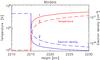 |
Fig. 1 Changes in the electron temperature (red) and density (blue) in two analyzed loop models. Numbers mark the model number. |
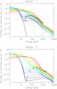 |
Fig. 2 Distribution functions at different positions in the transition-region along the loop in the Model 1 (top) and Model 2 (bottom). Different colors mark different distances along the loop model, and they are labeled by logarithm of temperature. Dashed lines correspond to the Maxwellian core of the distributions. |
2. Model transition region
Suprathermal transition region electron velocity distribution functions were calculated in Paper I by solving the Boltzmann-Vlasov equation including Coulomb collisions. This kinetic model is described in detail in Paper I. It is based on the coronal loop model of Vocks et al. (2008). The loop is 210 Mm long and its geometry is given by a potential extrapolation of a photospheric magnetogram observed on 2003 October 28. The loop has an apex temperature of 1.4 MK and a footpoint electron density of 2 × 109 cm-3. The new transition region simulation box is located below that of Vocks et al. (2008), and the electron distribution at the loop footpoint in Vocks et al. (2008) is used as an upper boundary condition for the transition region model.
This model requires a background fluid model, that is, densities and temperatures, for both electrons and ions in the transition region. The temperature profile is based on the classic Spitzer T5/2 law of thermal conductivity in a plasma, starting from the temperature at the upper boundary. The density profile is then calculated by a hydrostatic model.
In order to understand the effect of transition region thickness, a second model with an artificially thick transition region, based on a T3/2 law of thermal conductivity, has been prepared. The upper boundary conditions for density, temperature, and electron distribution, were not changed. This modification does not consider possible implications on the plasma state inside the loop, as they are discussed by Peter et al. (2012), for example.
From now on, the transition-region models based on the T5/2 and T3/2 thermal conductivity are simply referred to as Models 1 and 2, respectively. The resulting profiles of T and Ne are shown in Fig. 1. The increased thickness of the transition region in Model 2 can readily be seen, as the temperature reaches values of 1.0 × 10⁵ K or 2.0 × 10⁵ K, for example, at a larger height for Model 2 than for Model 1.
The resulting electron distributions as a function of energy are shown in Fig. 2 for both models. It can be seen that there are strong suprathermal tails present in the transition region, although the total numbers of the particles in the high-energy tails are small in comparison with the bulk of distribution in both Models. These high-energy tails arise as a result of collisionless particles streaming down the transition region from the hotter corona, where non-Maxwellian particle populations arose due to resonant interaction with the whistler waves, as discussed by Vocks et al. (2008).
The high-energy tails in Model 1 are typically approximately one order of magnitude higher than in the Model 2 for electron energies of several 10 eV up to a few 100 eV (Fig. 2 and Table 1). At higher electron energies, the difference becomes smaller, as electrons with such energies can traverse the transition region essentially collision-free. The relative number of the electrons in the high-energy tail reaches its maximum 4% at log(T) ≈ 4.6 for Model 1. It is important that these electrons carry approximately 25% of the total energy of the electron distribution (Table 1, left) and this energy source can have a significant effect on ionization and excitation. On the other hand, the relative number of the electrons in Model 2 is typically bellow 1% (Table 1, right). The high energy tail contains a few % of the total energy only and its effect is smaller than in Model 1.
The number of particles and their energy in the high-energy tail relative to the total particle number and the energy of the electron distribution for Model 1 (left) and Model 2 (right) as a function of temperature in the transition region.
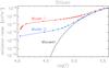 |
Fig. 3 Direct ionization rates as a function of temperature in the Model 1 (red), Model 2 (blue) and for the Maxwellian distribution (black). |
3. Synthetic spectra
Using the models described in Sect. 2, and especially the resulting distribution functions, we have calculated the ionization and excitation equilibrium, as well as the synthetic spectra for Si, O, and S at the spectral range 1390–1407 Å. This spectral range was chosen to model the transition region line emission observed by IRIS (IRIS, De Pontieu et al. 2014).
The line intensity I formed between levels i and j in the optically thin plasma is the integral of the emissivity, εij, along the line of sight 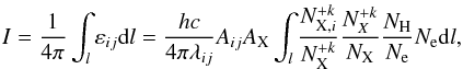 (1)where h is Planck constant, λij is the line wavelength corresponding to the transition from atomic level i to level j, Aij is the corresponding Einstein coefficient for spontaneous emission,
  is the number of ions with the excited level i,
  is the relative abundance of + k-times ionized ions to the total number of ions for element X, AX is the relative abundance of the element X to hydrogen, NH is the total number of hydrogen ions, and Ne is the electron density. In equilibrium, the ratio
  is given by the excitation equilibrium and is given by the ionization one.
3.1. Ionization equilibrium
In the high-temperature and low-density plasma, the electron direct ionization and autoionization together with radiative and dielectronic recombination are the dominant ionization and recombination processes. As such, they are important for the ionization equilibrium calculation. The rate of an elementary process for any energy distribution function, f(ℰ), can be written 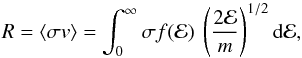 (2)where σ is the cross section, v is the electron velocity, and ℰ is the corresponding electron energy. The cross sections for the direct ionization and autoionization calculation were taken from the CHIANTI database, version 8.0 (Del Zanna et al. 2015). They correspond to atomic data of Dere (2007). Dere et al. (2009) used these data to calculate the ionization equilibria for the Maxwellian distribution. The ionization rates given by Eq. (2) for our model distributions have been calculated numerically. As a result of the presence of the high-energy tails of the distribution, the ionization rates show a strong increase at low temperatures (Fig. 3). The effect is more pronounced for Model 1 where more high-energy particles are present (see Fig. 2).
For the radiative recombination, we used the method of Dzifčáková (1992), Wannawichian et al. (2003), and Dzifčáková & Dudík (2013). Although this method was developed for the κ-distributions, it can be used for any distribution, including numerical ones. The cross-section for the radiative recombination, σRR, is assumed to have the form (e.g., Osterbrock 1974) 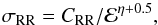 (3)where CRR is a constant and η + 0.5 is a power-law index. Both parameters can be found in Aldrovandi & Pequignot (1973), Landini & Monsignori Fossi (1990), Shull & van Steenberg (1982), Mazzotta et al. (1998), or Badnell (2006), for example. It should be noted that the recombination cross-section decreases with the incident energy and low-energy electrons are the main contributors to the radiative recombination rates. Therefore, the radiative recombination rates for our model distributions are nearly the same as the Maxwellian rates at temperatures corresponding to the distribution bulks. The small numbers of high-energy particles only have a minor effect on these rates (see also Roussel-Dupré 1980b).
Dielectronic recombination rates can be approximated by the following expression valid for any distribution function (Dzifčáková 1992; Dzifčáková & Dudík 2013) 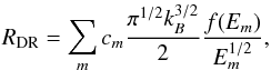 (4)where cm and Em are the parameters given by the approximations of the Maxwellian dielectronic recombination rates. We have taken data from Abdel-Naby et al. (2012), Aldrovandi & Pequignot (1973), Altun et al. (2004, 2006, 2007), Colgan et al. (2003, 2004), Mitnik & Badnell (2004), Zatsarinny et al. (2004, 2005a,b, 2006). These data are also part of the CHIANTI database since version 6 (see Dere et al. 2009).
In equilibrium, direct ionization and autoionization are compensated by the radiative with dielectronic recombination, leading to the following relation 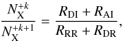 (5)where RDI is the rate of direct ionization and RAI is the rate of autoionization. The ionization equilibria for the model distributions were calculated in selected points along the loop. The abundace of Si ii–Si vi and O i–O vi ions as a function of temperature along the loop are shown in the Figs. 4 and 5. For comparison, relative abundances of the these ions for the Maxwellian distributions with the same temperatures are shown by dashed lines. It can be seen that the relative ion abundances are very sensitive to the presence of the high-energy tail. The ions in our models can exist in a wider temperature range in comparison with the Maxwellian case. In particular, the ions can also exist at very low temperatures. Furthermore, the maxima of the relative ion abundances are shifted to the lower temperatures. This shift is much stronger for the Model 1 where the number of high energy particles is higher. The behavior of the ionization peaks for our model distribution is, in general terms, similar to the effect of the κ-distributions on the ionization equilibrium in the transition region (Dzifčáková & Dudík 2013), although the details obtained here are different. The relative ion abundances calculated here show that even relatively weak non-Maxwellian tails in the transition region will have a significant impact on the ionization equilibrium, as also qualitatively discussed already by Roussel-Dupré (1980b).
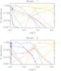 |
Fig. 4 Calculated Si ion abundances (full lines) for Model 1 (top) and Model 2 (bottom) in a comparison with the Maxwellian case (dashed lines). Different colors mark different ions and numbers correspond to the degree of ionization. |
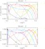 |
Fig. 5 Calculated O ion abundances (full lines) for Model 1 (top) and Model 2 (bottom) in a comparison with the Maxwellian case (dashed lines). Different colors mark different ions and numbers correspond to the degree of ionization. |
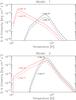 |
Fig. 6 Calculated emissivity of the strongest Si lines (red lines) for Model 1 (top) and Model 2 (bottom) in a comparison with the Maxwellian case (black lines). |
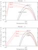 |
Fig. 7 Calculated emissivity of the strongest O lines (red lines) for Model 1 (top) and Model 2 (bottom) in a comparison with the Maxwellian case (black lines). |
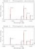 |
Fig. 8 Calculated synthetic spectrum observable in IRIS with the photospheric abundances (full red lines) for Model 1 (top) and Model 2 (bottom) in a comparison with the Maxwellian spectrum for the same temperature and density structure of the loop (dashed black lines). |
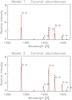 |
Fig. 9 Calculated synthetic spectrum observable in IRIS with the coronal abundances (full red lines) for Model 1 (top) and Model 2 (bottom) in a comparison with the Maxwellian spectrum for the same temperature and density structure of the loop (dashed black lines). |
3.2. Excitation equilibrium
In the solar transition region, the dominant processes are the electron collisional excitation and deexcitation together with the spontaneous radiative decay transitions. Photoexcitation can be negleted at the electron densities in our models (Dudík et al. 2014). Generally, the electron excitation rates are calculated from the non-dimensionalized collision strengths Ωij instead of the cross-sections σij themselves. These two quantities are related by 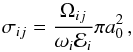 (6)where Eij is the excitation energy, ωi is the statistical weight of the level i, ℰi is the incident electron energy, IH is the hydrogen ionization energy, and a0 is the Bohr radius.
The CHIANTI database contains Maxwellian-averaged collision strengths or their spline approximations for the majority of the astronomically interesting ions of elements from H to Zn (Dere et al. 1997; Del Zanna et al. 2015). However, CHIANTI software enables calculation of spectra for the Maxwellian plasma only. Consequently, Dzifčáková et al. (2015) developed a method to calculate Ω for the approximate excitation and de-excitation rates for non-Maxwellian distributions. They tested and applied this method for the κ-distributions and showed that the approximate method yields collisional excitation rates within 5–10% compared to the direct numerical calculations. These approximations of Ω are contained in the KAPPA package (Dzifčáková et al. 2015). For our model distributions (Sect. 2), we used these approximations to calculate excitation equilibria and synthetic spectra of Si iv, O iv, and S iv in the IRIS FUV wavelength window. These calculations are based on the atomic data of Liang et al. (2009a), Liang et al. (2009b), Feuchtgruber et al. (1997), Liang et al. (2012), Correge & Hibbert (2004), Foster et al. (1997), Tayal (2000), Tayal (1999), Hibbert et al. (2002), Johnson et al. (1986), and Bely & Faucher (1970).
3.3. Line intensities
Having obtained the ionization and excitation equilibria (Sects. 3.1 and 3.2, respectively), we next calculated the emissivities of the Si iv and O iv lines for both models. Since the amount of high-energy particles present in the model transition region is small (Sect. 2 and Table 1) despite their effects on ionization equilibrium, the synthetic spectra obtained here are compared with the Maxwellian ones. We remind the reader that the Maxwellian spectra typically show higher O iv 1401.2 Å intensities compared to Si iv 1402.8 Å ones. This is contrary to the observed spectra, where Si iv is enhanced compared to O iv, by a factor of five or more. Thus, rather than reproducing the observed spectra in detail, our aim here is only to investigate the effect (if any) of the non-Maxwellian particles within Models 1 and 2 on the emergent transition region spectra.
The calculated emissivities of Si iv and O iv lines for both models are shown in Figs. 6 and 7. It can be seen that even a small number of high-energy particles results in the enhancement of emissivity by several orders at temperatures close to 104 K for Model 2. Both the Si iv and O iv contribution functions have a pronounced wing towards temperatures as low as 3 × 10⁴ K. Increase of the high-energy particles in Model 1 results in formation of Si iv and O iv emissivity maxima at temperatures of approximately 1.5 × 10⁴ K, which is approximately one order of magnitude lower than the temperature of emissivity maxima in the Maxwellian case, and also significantly lower than in Model 2.
The synthetic spectra in the IRIS FUV channel are shown in red in Figs. 8 and 9, where the corresponding Maxwellian spectra are also shown by black dashed lines. The spectra are integrated along the model atmosphere shown in Fig. 1. This is since the transition region here corresponds to a footpoint of a coronal loop (Paper I) rather than a purely transition-region structure such as a small loop. While the synthetic spectra are obtained by using the full modeled distribution functions (Fig. 2), the corresponding Maxwellian spectra are obtained using only the Maxwellian cores of the distribution at each location. Finally, the spectra shown in Fig. 8 were obtained using the photospheric abundances (Asplund et al. 2009), while those in Fig. 9 correspond to the coronal abundances (Feldman et al. 1992).
The synthetic spectra reflect the behavior of the emissivities shown in Figs. 6 and 7. For Model 2, the resulting spectrum is similar to the Maxwellian spectrum (Figs. 8 and 9, bottom); however, the O iv intensities are weakly enhanced compared to the Maxwellian, while the Si iv are depressed by around 20–30%. The S iv is almost unaffected. Such changes in the O iv and Si iv intensities depart further from the typically observed spectra. Thus, Model 2 does not help in reducing the discrepancy between the synthetic and observed Si iv and O iv intensities.
On the other hand, for Model 1, the Si iv 1402.8 Å line is increased by more than a factor of 2 compared to the Maxwellian case, while the O iv intensities are depleted by several tens of per cent (Table 2 and top panels in Figs. 8, 9). This behavior is qualitatively similar to the effect of the κ-distribution on the IRIS spectra (Dudík et al. 2014). In our case however, the decrease of O iv relative to Si iv is not so pronounced, and the Si iv to O iv intensity ratios change only by approximately a factor of 2. This comes from the much weaker high-energy tail in our model distribution (Fig. 2) compared to a κ-distribution. Nevertheless, the spectra obtained for Model 1 help to reduce the discrepancy between the synthetic Maxwellian and the actually observed ones. This shows that even a relatively small number of energetic particles, generated with a simple model of the transition region, can still have a significant effect on the emergent spectra.
Relative intensities of O iv 1401.16 Å and 1399.77 Å line to Si iv 1393.76 Å line for Model 1(left) and Model 2 (right) assuming photospheric and coronal abundances.
4. Summary and discussion
We calculated the synthetic transition-region spectra emerging from the transition region model of Paper I. This model considers the propagation of particles in the transition region below a coronal loop, where high-energy tails are created by whistler-wave turbulence (Vocks et al. 2008). The high-energy tails are relatively weak, containing less than 4% of the particles. These high-energy tails enhance the ionization rates, which show pronounced low-temperature shoulders. Consequently, ions such as Si iii–Si v and O iii–O v exist also at very low temperatures almost down to 104 K. This behavior is in turn translated to the behavior of the contribution functions of the Si iv and O iv lines observed by IRIS. The resulting synthetic spectra for the Model 1 show increase of the Si iv intensities by a factor of more than 2, while the O iv lines are weakly decreased when compared to the corresponding Maxwellian spectra. For Model 2, the O iv lines are weakly enhanced as a result of their contribution functions being more flat at transition region temperatures than the Si iv ones.
We note that in both cases, the synthetic spectra obtained here still contain O iv 1401.2 Å intensities comparable to the Si iv 1402.8 Å ones, while in observations, the Si iv intensities are much larger. Transient ionization has been shown to strongly affect the Si iv and O iv intensities. The spectra calculated from models of solar atmosphere, including transient ionization (e.g., Doyle et al. 2013; Olluri et al. 2013b,a; Martínez-Sykora et al. 2016), show enhancements of Si iv relative to O iv similar to observations. Although the importance of the transient ionization is beyond reasonable doubt, our results show that the propagation of high-energy particles through the transition region also needs to be considered as it can also lead to enhancements of the Si iv lines and weak depletions of the O iv ones when compared to the equilibrium Maxwellian spectrum. We note that the high-energy tails considered here occur naturally in the transition region. Thus, these high-energy tails exist even outside reconnection events or strong electric fields, which would likely increase the high-energy tails and further modify the emergent spectrum.
Acknowledgments
This work has been supported by Grant Nos. 16-18495S and 17-16447S of the Grant Agency of the Czech Republic. We used the CHIANTI software and database. CHIANTI is a collaborative project involving the NRL (USA), RAL (UK), MSSL (UK), the Universities of Florence (Italy) and Cambridge (UK), and George Mason University (USA). The authors benefited greatly from participation in the International Team 276 funded by the International Space Science Institute (ISSI) in Bern, Switzerland.
References
- Abdel-Naby, S. A., Nikolić, D., Gorczyca, T. W., Korista, K. T., & Badnell, N. R. 2012, A&A, 537, A40 [NASA ADS] [CrossRef] [EDP Sciences] [Google Scholar]
- Aldrovandi, S. M. V., & Pequignot, D. 1973, A&A, 25, 137 [NASA ADS] [Google Scholar]
- Altun, Z., Yumak, A., Badnell, N. R., Colgan, J., & Pindzola, M. S. 2004, A&A, 420, 775 [NASA ADS] [CrossRef] [EDP Sciences] [Google Scholar]
- Altun, Z., Yumak, A., Badnell, N. R., Loch, S. D., & Pindzola, M. S. 2006, A&A, 447, 1165 [NASA ADS] [CrossRef] [EDP Sciences] [Google Scholar]
- Altun, Z., Yumak, A., Yavuz, I., et al. 2007, A&A, 474, 1051 [NASA ADS] [CrossRef] [EDP Sciences] [Google Scholar]
- Asplund, M., Grevesse, N., Sauval, A. J., & Scott, P. 2009, ARA&A, 47, 481 [NASA ADS] [CrossRef] [Google Scholar]
- Badnell, N. R. 2006, ApJS, 167, 334 [NASA ADS] [CrossRef] [Google Scholar]
- Bely, O., & Faucher, P. 1970, A&A, 6, 88 [NASA ADS] [Google Scholar]
- Bradshaw, S. J., & Cargill, P. J. 2013, ApJ, 770, 12 [NASA ADS] [CrossRef] [Google Scholar]
- Colgan, J., Pindzola, M. S., Whiteford, A. D., & Badnell, N. R. 2003, A&A, 412, 597 [NASA ADS] [CrossRef] [EDP Sciences] [Google Scholar]
- Colgan, J., Pindzola, M. S., & Badnell, N. R. 2004, A&A, 417, 1183 [NASA ADS] [CrossRef] [EDP Sciences] [Google Scholar]
- Correge, G., & Hibbert, A. 2004, Atom. Data Nucl. Data Tables, 86, 19 [NASA ADS] [CrossRef] [Google Scholar]
- Curdt, W., Brekke, P., Feldman, U., et al. 2001, A&A, 375, 591 [NASA ADS] [CrossRef] [EDP Sciences] [Google Scholar]
- Del Zanna, G., Dere, K. P., Young, P. R., Landi, E., & Mason, H. E. 2015, A&A, 582, A56 [NASA ADS] [CrossRef] [EDP Sciences] [Google Scholar]
- De Pontieu, B., Title, A. M., Lemen, J. R., et al. 2014, Sol. Phys., 289, 2733 [NASA ADS] [CrossRef] [Google Scholar]
- Dere, K. P. 2007, A&A, 466, 771 [NASA ADS] [CrossRef] [EDP Sciences] [Google Scholar]
- Dere, K. P., Landi, E., Mason, H. E., Monsignori Fossi, B. C., & Young, P. R. 1997, A&AS, 125 [Google Scholar]
- Dere, K. P., Landi, E., Young, P. R., et al. 2009, A&A, 498, 915 [NASA ADS] [CrossRef] [EDP Sciences] [Google Scholar]
- Doschek, G. A., Warren, H. P., & Young, P. R. 2016, ApJ, 832, 77 [NASA ADS] [CrossRef] [Google Scholar]
- Doyle, J. G., & Raymond, J. C. 1984, Sol. Phys., 90, 97 [NASA ADS] [CrossRef] [Google Scholar]
- Doyle, J. G., Giunta, A., Madjarska, M. S., et al. 2013, A&A, 557, L9 [NASA ADS] [CrossRef] [EDP Sciences] [Google Scholar]
- Dudík, J., Del Zanna, G., Dzifčáková, E., Mason, H. E., & Golub, L. 2014, ApJ, 780, L12 [NASA ADS] [CrossRef] [Google Scholar]
- Dupree, A. K. 1972, ApJ, 178, 527 [NASA ADS] [CrossRef] [Google Scholar]
- Dzifčáková, E. 1992, Sol. Phys., 140, 247 [NASA ADS] [CrossRef] [Google Scholar]
- Dzifčáková, E., & Dudík, J. 2013, ApJS, 206, 6 [NASA ADS] [CrossRef] [Google Scholar]
- Dzifčáková, E., Dudík, J., Kotrč, P., Fárník, F., & Zemanová, A. 2015, ApJS, 217, 14 [NASA ADS] [CrossRef] [Google Scholar]
- Feldman, U., Mandelbaum, P., Seely, J. F., Doschek, G. A., & Gursky, H. 1992, ApJS, 81, 387 [NASA ADS] [CrossRef] [Google Scholar]
- Feuchtgruber, H., Lutz, D., Beintema, D. A., et al. 1997, ApJ, 487, 962 [NASA ADS] [CrossRef] [Google Scholar]
- Fontenla, J. M., Avrett, E. H., & Loeser, R. 1990, ApJ, 355, 700 [NASA ADS] [CrossRef] [Google Scholar]
- Fontenla, J. M., Avrett, E. H., & Loeser, R. 1991, ApJ, 377, 712 [NASA ADS] [CrossRef] [Google Scholar]
- Fontenla, J. M., Avrett, E. H., & Loeser, R. 1993, ApJ, 406, 319 [NASA ADS] [CrossRef] [Google Scholar]
- Foster, V. J., Keenan, F. P., & Reid, R. H. G. 1997, Atom. Data Nucl. Data Tables, 67, 99 [Google Scholar]
- Gudiksen, B. V., & Nordlund, Å. 2005a, ApJ, 618, 1031 [NASA ADS] [CrossRef] [Google Scholar]
- Gudiksen, B. V., & Nordlund, Å. 2005b, ApJ, 618, 1020 [NASA ADS] [CrossRef] [Google Scholar]
- Hansteen, V., Guerreiro, N., De Pontieu, B., & Carlsson, M. 2015, ApJ, 811, 106 [NASA ADS] [CrossRef] [Google Scholar]
- Hibbert, A., Brage, T., & Fleming, J. 2002, MNRAS, 333, 885 [NASA ADS] [CrossRef] [Google Scholar]
- Johnson, C. T., Kingston, A. E., & Dufton, P. L. 1986, MNRAS, 220, 155 [NASA ADS] [CrossRef] [Google Scholar]
- Judge, P. G., Woods, T. N., Brekke, P., & Rottman, G. J. 1995, ApJ, 455, L85 [NASA ADS] [CrossRef] [Google Scholar]
- Landini, M., & Monsignori Fossi, B. C. 1990, A&AS, 82, 229 [NASA ADS] [Google Scholar]
- Liang, G. Y., Whiteford, A. D., & Badnell, N. R. 2009a, A&A, 500, 1263 [NASA ADS] [CrossRef] [EDP Sciences] [Google Scholar]
- Liang, G. Y., Whiteford, A. D., & Badnell, N. R. 2009b, J. Phys. B At. Mol. Phys., 42, 225002 [NASA ADS] [CrossRef] [Google Scholar]
- Liang, G. Y., Badnell, N. R., & Zhao, G. 2012, A&A, 547, A87 [NASA ADS] [CrossRef] [EDP Sciences] [Google Scholar]
- Ljepojevic, N. N., & MacNeice, P. 1988, Sol. Phys., 117, 123 [NASA ADS] [CrossRef] [Google Scholar]
- Martínez-Sykora, J., De Pontieu, B., Hansteen, V. H., & Gudiksen, B. 2016, ApJ, 817, 46 [NASA ADS] [CrossRef] [Google Scholar]
- Mazzotta, P., Mazzitelli, G., Colafrancesco, S., & Vittorio, N. 1998, A&AS, 133, 403 [Google Scholar]
- Mitnik, D. M., & Badnell, N. R. 2004, A&A, 425, 1153 [NASA ADS] [CrossRef] [EDP Sciences] [Google Scholar]
- Olluri, K., Gudiksen, B. V., & Hansteen, V. H. 2013a, ApJ, 767, 43 [NASA ADS] [CrossRef] [Google Scholar]
- Olluri, K., Gudiksen, B. V., & Hansteen, V. H. 2013b, AJ, 145, 72 [NASA ADS] [CrossRef] [Google Scholar]
- Osterbrock, D. E. 1974, Astrophysics of gaseous nebulae (San Francisco; W.H. Freeman and Co) [Google Scholar]
- Peter, H., Bingert, S., & Kamio, S. 2012, A&A, 537, A152 [NASA ADS] [CrossRef] [EDP Sciences] [Google Scholar]
- Peter, H., Tian, H., Curdt, W., et al. 2014, Science, 346, 1255726 [NASA ADS] [CrossRef] [Google Scholar]
- Polito, V., Del Zanna, G., Dudík, J., et al. 2016, A&A, 594, A64 [NASA ADS] [CrossRef] [EDP Sciences] [Google Scholar]
- Roussel-Dupré, R. 1980a, Sol. Phys., 68, 243 [NASA ADS] [CrossRef] [Google Scholar]
- Roussel-Dupré, R. 1980b, Sol. Phys., 68, 265 [NASA ADS] [CrossRef] [Google Scholar]
- Shoub, E. C. 1983, ApJ, 266, 339 [NASA ADS] [CrossRef] [Google Scholar]
- Shull, J. M., & van Steenberg, M. 1982, ApJS, 48, 95 [NASA ADS] [CrossRef] [Google Scholar]
- Tayal, S. S. 1999, J. Phys. B: At., Mol. Opt. Phys., 32, 5311 [Google Scholar]
- Tayal, S. S. 2000, ApJ, 530, 1091 [NASA ADS] [CrossRef] [Google Scholar]
- Testa, P., De Pontieu, B., Allred, J., et al. 2014, Science, 346, 1255724 [NASA ADS] [CrossRef] [Google Scholar]
- Vocks, C., Mann, G., & Rausche, G. 2008, A&A, 480, 527 [NASA ADS] [CrossRef] [EDP Sciences] [Google Scholar]
- Vocks, C., Dzifčáková, E., & Mann, G. 2016, A&A, 596, A41 [NASA ADS] [CrossRef] [EDP Sciences] [Google Scholar]
- Wannawichian, S., Ruffolo, D., & Kartavykh, Y. Y. 2003, ApJS, 146, 443 [NASA ADS] [CrossRef] [Google Scholar]
- Yan, L., Peter, H., He, J., et al. 2015, ApJ, 811, 48 [NASA ADS] [CrossRef] [Google Scholar]
- Zatsarinny, O., Gorczyca, T. W., Korista, K., Badnell, N. R., & Savin, D. W. 2004, A&A, 426, 699 [NASA ADS] [CrossRef] [EDP Sciences] [Google Scholar]
- Zatsarinny, O., Gorczyca, T. W., Korista, K. T., et al. 2005a, A&A, 438, 743 [NASA ADS] [CrossRef] [EDP Sciences] [Google Scholar]
- Zatsarinny, O., Gorczyca, T. W., Korista, K. T., et al. 2005b, A&A, 440, 1203 [NASA ADS] [CrossRef] [EDP Sciences] [Google Scholar]
- Zatsarinny, O., Gorczyca, T. W., Fu, J., et al. 2006, A&A, 447, 379 [NASA ADS] [CrossRef] [EDP Sciences] [Google Scholar]
All Tables
The number of particles and their energy in the high-energy tail relative to the total particle number and the energy of the electron distribution for Model 1 (left) and Model 2 (right) as a function of temperature in the transition region.
Relative intensities of O iv 1401.16 Å and 1399.77 Å line to Si iv 1393.76 Å line for Model 1(left) and Model 2 (right) assuming photospheric and coronal abundances.
All Figures
|
Fig. 1 Changes in the electron temperature (red) and density (blue) in two analyzed loop models. Numbers mark the model number. |
| In the text | |
|
Fig. 2 Distribution functions at different positions in the transition-region along the loop in the Model 1 (top) and Model 2 (bottom). Different colors mark different distances along the loop model, and they are labeled by logarithm of temperature. Dashed lines correspond to the Maxwellian core of the distributions. |
| In the text | |
|
Fig. 3 Direct ionization rates as a function of temperature in the Model 1 (red), Model 2 (blue) and for the Maxwellian distribution (black). |
| In the text | |
|
Fig. 4 Calculated Si ion abundances (full lines) for Model 1 (top) and Model 2 (bottom) in a comparison with the Maxwellian case (dashed lines). Different colors mark different ions and numbers correspond to the degree of ionization. |
| In the text | |
|
Fig. 5 Calculated O ion abundances (full lines) for Model 1 (top) and Model 2 (bottom) in a comparison with the Maxwellian case (dashed lines). Different colors mark different ions and numbers correspond to the degree of ionization. |
| In the text | |
|
Fig. 6 Calculated emissivity of the strongest Si lines (red lines) for Model 1 (top) and Model 2 (bottom) in a comparison with the Maxwellian case (black lines). |
| In the text | |
|
Fig. 7 Calculated emissivity of the strongest O lines (red lines) for Model 1 (top) and Model 2 (bottom) in a comparison with the Maxwellian case (black lines). |
| In the text | |
|
Fig. 8 Calculated synthetic spectrum observable in IRIS with the photospheric abundances (full red lines) for Model 1 (top) and Model 2 (bottom) in a comparison with the Maxwellian spectrum for the same temperature and density structure of the loop (dashed black lines). |
| In the text | |
|
Fig. 9 Calculated synthetic spectrum observable in IRIS with the coronal abundances (full red lines) for Model 1 (top) and Model 2 (bottom) in a comparison with the Maxwellian spectrum for the same temperature and density structure of the loop (dashed black lines). |
| In the text | |
Current usage metrics show cumulative count of Article Views (full-text article views including HTML views, PDF and ePub downloads, according to the available data) and Abstracts Views on Vision4Press platform.
Data correspond to usage on the plateform after 2015. The current usage metrics is available 48-96 hours after online publication and is updated daily on week days.
Initial download of the metrics may take a while.