| Issue |
A&A
Volume 602, June 2017
|
|
|---|---|---|
| Article Number | A29 | |
| Number of page(s) | 27 | |
| Section | Extragalactic astronomy | |
| DOI | https://doi.org/10.1051/0004-6361/201629999 | |
| Published online | 30 May 2017 | |
A swirling jet in the quasar 1308+326⋆
1 Max-Planck-Institut für Radioastronomie, Auf dem Hügel 69, 53121 Bonn, Germany
e-mail: sbritzen@mpifr.de
2 National Astronomical Observatories, Chinese Academy of Sciences, 100012 Beijing, PR China
3 Instituto de Astronomía, Universidad Nacional Autónoma de México, 22800 Ensenada, B.C., Mexico
4 Physics Institute, University of Szeged, Dóm tér 9, 6720 Szeged, Hungary
5 Astronomy Program, Department of Physics & Astronomy, Seoul National University, Gwanak-gu, 151-742 Seoul, Republic of Korea
6 Nature Astronomy, Springer Nature, 4 Crinan Street, N1 9XW, London, UK
7 University of Michigan, Ann Arbor, MI 48109, USA
8 Max-Planck-Institut für Astronomie, Königstuhl, 69117 Heidelberg, Germany
9 Centre for Space Research, North-West University, 2520 Potchefstroom, South Africa
10 Universität zu Köln, Zülpicher Strasse 77, 50937 Köln, Germany
11 Argelander-Institut für Astronomie, Universität Bonn, Auf dem Hügel 71, 53121 Bonn, Germany
Received: 2 November 2016
Accepted: 13 February 2017
Context. Despite numerous and detailed studies of the jets of active galactic nuclei (AGN) on pc-scales, many questions are still debated. The physical nature of the jet components is one of the most prominent unsolved problems, as is the launching mechanism of jets in AGN. The quasar 1308+326 (z = 0.997) allows us to study the overall properties of its jet in detail and to derive a more physical understanding of the nature and origin of jets in general. The long-term data provided by the Monitoring Of Jets in Active galactic nuclei with Very Long Baseline Array (VLBA) experiments (MOJAVE)⋆⋆ survey permit us to trace out the structural changes in 1308+326 that we present here. The long-lived jet features in this source can be followed for about two decades.
Aims. We investigate the very long baseline interferomety (VLBI) morphology and kinematics of the jet of 1308+326 to understand the physical nature of this jet and jets in general, the role of magnetic fields, and the causal connection between jet features and the launching process.
Methods. Fifty VLBA observations performed at 15 GHz from the MOJAVE survey were re-modeled with Gaussian components and re-analyzed (the time covered: 20 Jan. 1995–25 Jan. 2014). The analysis was supplemented by multi-wavelength radio-data (UMRAO, at 4.8, 8.0, and 14.5 GHz) in polarization and total intensity. We fit the apparent motion of the jet features with the help of a model of a precessing nozzle.
Results. The jet features seem to be emitted with varying viewing angles and launched into an ejection cone. Tracing the component paths yields evidence for rotational motion. Radio flux-density variability can be explained as a consequence of enhanced Doppler boosting corresponding to the motion of the jet relative to the line of sight. Based on the presented kinematics and other indicators, such as electric-vector polarization position-angle (EVPA) rotation, we conclude that the jet of 1308+326 has a helical structure, meaning that the components are moving along helical trajectories and the trajectories themselves are also experiencing a precessing motion. A model of a precessing nozzle was applied to the data and a subset of the observed jet feature paths can be modeled successfully within this model. The data till 2012 are consistent with a swing period of 16.9 yr. We discuss several scenarios to explain the observed motion phenomena, including a binary black hole model. It seems unlikely that the accretion disk around the primary black hole, which is disturbed by the tidal forces of the secondary black hole, is able to launch a persistent axisymmetric jet.
Conclusions. We conclude that we are observing a rotating helix. In particular, the observed EVPA swings can be explained by a shock moving through a straight jet that is pervaded by a helical magnetic field. We compare our results for 1308+326 with other astrophysical scenarios where similar, wound-up filamentary structures are found. They are all related to accretion-driven processes. A helically moving or wound up object is often explained by filamentary features moving along magnetic field lines of magnetic flux tubes. It seems that a “component” comprises plasma tracing the magnetic field, which guides the motion of the radiating radio-band plasma. Further investigations and modeling are in preparation.
Key words: quasars: general / techniques: interferometric
The reduced Figs. A.1–A.13 (FITS files) are only available at the CDS via anonymous ftp to cdsarc.u-strasbg.fr (130.79.128.5) or via http://cdsarc.u-strasbg.fr/viz-bin/qcat?J/A+A/602/A29
© ESO, 2017
1. Introduction
Many aspects regarding parsec-scale jets in active galactic nuclei (AGN) are still debated. Hundreds of AGN jets have been investigated with available high-resolution interferometric arrays and the whole span of radio frequencies was explored. Still it is not clear what jets are made of (e.g., Böttcher et al. 2015), or how they are launched (e.g., Blandford & Payne 1982; Blandford & Znajek 1977). There is some progress with regard to the first question, and the expected improved resolution of observations with the Event Horizon Telescope (e.g., Doeleman 2010) might help to answer the second question. Related to the latter is the question of the role of the magnetic fields in the accretion disc with regard to the jet launching, and in the jet with regard to collimation and acceleration. Another unsolved question is related to what jet components are. The term “component” refers to inhomogeneities in the jet brightness distribution and is used because it is unclear what the physical origin of the observed bright features in jets is. To name the most important concepts: shocks (e.g., Marscher & Gear 1985), instabilities (e.g. Hardee 2011), and sites of enhanced Doppler boosting due to geometrical effects (e.g., Camenzind & Krockenberger 1992). Much work was performed in investigating the evolution of the core separation of the individual jet components with time. However, the detailed analysis of both projected coordinates shows that jet component motion is a complex phenomenon and not restricted to simple outward motion (e.g., Britzen et al. 2010; Karouzos et al. 2012; Cohen et al. 2015).
2. Radio interferometric observations of 1308+326
The source classification of 1308+326 changed from BL Lac Object to quasar (see text later on), and currently it is classified as a low-synchrotron peaked (LSP) high polarization quasar (HPQ). The large scale radio-structure of 1308+326 as shown in Fig. 1 (top) in a VLA observation by Cassaro et al. (1999), indicates a strongly curved jet. 1308+326 was classified both as a BL Lac object (e.g., Gabuzda et al. 1993) and as a quasar (e.g., Carrasco et al. 2012). Gabuzda et al. (1993) discuss the question of the proper classification of this source. According to them, the BL Lac classification is based on its nearly featureless optical continuum spectrum and high and variable polarization. They claim that the finding of both VLBI polarization structure and tentative superluminal motion is more characteristic for quasars. By analyzing polarization-sensitive VLBI observations of BL Lac objects, the authors find that for 1308+326 intrinsic structures can clearly be seen in the observations interpreted as core and the innermost knot. Surprising to the authors, a large offset angle between the jet direction and its polarization angle was found, similar to those of quasars.
1308+326 was studied as part of the MOJAVE1 survey (e.g., Hovatta et al. 2014; Lister et al. 2009a, 2013). The source shows a typical core-jet structure with the generally observed apparent superluminal motion. The source is also part of the catalog of radio reference frame sources of geodetic very long baseline interferometry (VLBI; ICRF, Ma et al. 1998, 2009; Jacobs et al. 2014) and was investigated by Piner et al. (2012). The reason for us picking this source and performing a detailed analysis of the VLBI structure and kinematics was to clarify the reason for unusual astrometric position instabilities (e.g., Bouffet et al. 2012) that could not be easily explained with simple and generally assumed outward motion of jet components. The standard model for astrometric position instabilities is that jet components separate from the core and cause shifts of the brightness centroid.
 |
Fig. 1 B-array VLA image obtained at 1.46 GHz by Cassaro et al. (1999). |
3. Multi-wavelength observations of 1308+326
1308+326 was observed various times in the last decades due to its prominent outbursts and due to its ambiguous classification between a BL Lac object and a quasar. Along with the question on the proper classification of this source come more general discussions on whether quasars and BL Lac objects reveal different polarization properties (e.g., Gabuzda & Cawthorne 1992; Pudritz et al. 2012) and whether the magnetic fields are parallel (quasars) or orthogonal (BL Lac objects) to the jet axis. Because we (briefly) discuss the kinematics as well as the polarization properties of 1308+326 in this paper, we document the literature on the debate of the classification problem.
An early note by Liller et al. (1976) reported outbursts of 1308+326 measured in the optical back to 1940, 1974, and 1975. The outbursts reached magnitudes up to mB = 14.2 for the normally faint object of mB ~ 18.0.
In early 1977, a major outburst of 1308+326 was detected (Puschell et al. 1979). Photometric measurements were accomplished in the visual, infrared, millimeter, and centimeter range by Puschell et al. (1979). They found a high polarization over all observed wavelengths, whereas the visual polarization changed on a timescale of 15 min during the outburst. Polarization and photometric measurements in the visual and infrared wavebands for this outburst were also obtained by Moore et al. (1980). They also found a high degree of polarization and strong variations of the position angles during this period. From 1976 to 1983, 1308+326 was monitored by Mufson et al. (1983) in the visual waveband using photometry (UBVRI), and in the radio waveband at two frequencies (14.5, 8.0 GHz) within the UMRAO monitoring program. During this period, Mufson et al. (1983) found the object to be highly variable and active with periodic-like outbursts on a one year timescale. A correlation between the optical and radio outburst was described as marginal.
Contemporaneous observations at X-ray, optical, and radio wavelengths were published (Watson et al. 2000). The authors found the source showing features of a radio-selected BL (RBL) Lac object as well as features of a quasar. The object 1308+326 was at that time observed with resolutions that did not reveal the intrinsic structure as a core and knots of jets. During the X-ray observations, a non-variable low synchrotron flux was observed, in contrast to a much higher flux measured during previous ROSAT observations. The X-ray spectrum could be explained by a synchrotron emission at lower energies and inverse Compton emission at higher energies. Again, the question of whether this source can be classified as quasar or BL Lac Object was raised. The authors conclude that based on its high bolometric luminosity, variable line emission, and high Doppler boost factor it appears more like a quasar. Watson et al. (2000) also detect absorption at a level in excess of the Galactic value and conclude that a foreground absorber might be present and a gravitational microlensing scenario cannot be ruled out. This lensing option had already been discussed by Gabuzda et al. (1993) and Stickel et al. (1991).
The object 1308+326 is also detected by the Fermi-LAT instrument in the gamma-ray regime (Ackermann et al. 2013). A near-infrared (NIR) observation published in 2012 (Carrasco et al. 2012) showed again a significant flux variation over a period of more than one year. The source is currently designated as QSO.
This paper is organized as follows: Sect. 2 describes the data reduction, Sect. 3 presents the results of the data analysis and the results of modeling the data within a precessing nozzle scenario. Section 4 discusses the implications derived from the data results and modeling and we summarize the main findings in the conclusions in Sect. 5. Throughout the paper we used the recently determined cosmological parameters by the Planck mission (Planck Collaboration XIII 2016) according to which the angular scale is 1 mas = 0.008 pc.
4. Observations and data reduction
The MOJAVE survey provides access to excellent Very Long Baseline Array (VLBA) data taken at 15 GHz. This is of great value for investigating AGN properties on a statistical basis (e.g., Lister et al. 2016; Homan et al. 2015). Whereas the MOJAVE team is providing a statistical analysis of the complete sample, our approach is to select and focus on specific sources which appear to be special due to unique or rare properties. Although a statistical analysis of large numbers of sources is certainly of utmost importance and great value, a detailed analysis concentrating on peculiar properties – that are not necessarily common to the AGN population – can produce complementary results. We re-modeled fifty VLBA observations of 1308+326 obtained at 15 GHz (taken from the online MOJAVE archive webpage) between 1995.05 and 2014.07 with Gaussian components within the difmap-modelfit program (Shepherd 1997). The modelfit program fits image-plane model components to the visibilities in the uv plane. We did not apply self-calibration but used the calibration as provided by the MOJAVE team. Only circular components were used. The use of exclusively circular Gaussian components proved to be the most efficient way to parameterize the component properties. It reduces the number of free parameters, compared to the use of elliptical Gaussians, and allows a more secure identification of components across the epochs. Although it might have advantages to model the data of some of the epochs with elliptical components, our experience is that circular component modeling allows a more homogeneous analysis of all the epochs and more trustworthy identification of individual components in their long-term motion and evolution. Every epoch was modeled independently starting from a point source model. The errors were estimated from deviations in all parameters derived by calculating fits to models with ±1 component. All the images with model-fits superimposed are displayed in Figs. A.1–A.13. The parameters and corresponding uncertainties of the model-fits are listed in Table A.1. Components labeled with an “x” denote the presence of features that could not be reliably traced across the epochs. In addition we analyzed single-dish total intensity and polarization radio monitoring data at three radio frequencies, which was observed by the UMRAO monitoring program.
5. Results
5.1. Difference between VLA- and VLBI-scale jet orientations
The VLA map in Fig. 1 shows the kpc-scale jet emission of 1308+326 as observed by Cassaro et al. (1999). Obviously, the direction of the VLBI-jet emission as shown in Figs. A.1–A.13 is different. The kpc-scale emission is pointing toward the east and the north. On pc-scales, based on the 15 GHz observations, the VLBI jet is pointing roughly in the opposite, western, direction. Projection effects might play an important role assuming that the quasar is viewed under a small angle (e.g., Appl et al. 1996). A viewing angle of 3.6 deg and a Doppler factor of 22.0 were determined by Pushkarev et al. (2009). The viewing angle was determined on the basis of the MOJAVE VLBI observations and kinematic analysis. The Doppler factor was derived based on the results of the Metsähovi AGN monitoring program.
5.2. VLBI-scale jet
The most obvious result of our investigations of this source is the significant morphological evolution of the pc-scale jet with time. In Fig. 2 we show a subset of the images re-analyzed for this manuscript. From the earliest image shown (taken in January 1995) to the last image shown (2008.54) a significant evolution of the jet is visible. The composite image reveals the apparent structural evolution. From a point-like source the pc-scale jets develops and shapes into a more and more clearly visible helical structure. Figures A.1–A.13 display all fifty VLBI images with their Gaussian components superimposed.
 |
Fig. 2 Composite image of several selected VLBI images superimposed by Gaussian modelfit components. The dates of the 15 GHz observations are indicated in the plot. The core position is marked by the light blue line for better comparison. For the scale: in the last image (2008.54) the inner 6 mas are shown. We note that this is a subsample of the total of fifty observations re-modeled and re-analyzed in the paper. The complete set of images can be found in Appendix A. The contour levels shown here are listed in the following notation: lowest level (in percentage of the peak flux) and first positive level (in percentage of the peak flux), highest level (in percentage of the peak flux), and the scale factor between subsequent levels. The contour levels are: –0.6%, 76.8%, 2 (1995.05); –0.3%, 76.8%, 2 (1999.01); –0.5%, 59.3%, 1.7 (2000.06); –0.5%, 59.3%, 1.7 (2000.07); –0.3%, 52.8%, 1.6 (2000.49); –0.7%, 48.8%, 1.7 (2001.00); –0.2%, 51.2%, 2 (2001.65); –0.2%, 51.2%, 2 (2002.65); –0.2%; 51.2%, 2 (2002.90); –0.3%; 76.8%; 2 (2006.52); –0.1%, 51,2%, 2 (2008.41); –0.1%, 58.3%, 17 (2008.54). |
5.3. Apparent superluminal motion appears bundled
Our analysis reveals outward directed motion of jet features. This kind of motion is typical for quasars. For those components that can be identified and traced over a sufficiently long time span, we determine the apparent speeds (see Fig. 3, left). We list the values for proper motions, βapp, and the estimated times of ejection in Table 1. The apparent speeds are comparable with those values determined for quasars in several surveys (e.g., CJF: Britzen et al. 2008; MOJAVE: Lister et al. 2009a) and vary for different jet features of 1308+326 between values of 2.6c and 12.6c. Interestingly, the apparent speeds appear bundled, for example in groups rather than as a random mix of high and low apparent speeds. We find slow speeds for b, high speeds for c, d, and e; low speeds for f, g, and h; higher speeds again for i and j. For a and k the number of data points is not sufficient to check this. There are longer phases between the appearance of these bundled components in which no component ejection can be detected. To our knowledge, both findings are atypical. Component ejection seems to be a more regular phenomenon in typical quasars, and times without component ejections usually are not so pronounced. Lister et al. (2013) analyze the kinematics of two hundred parsec-scale AGN jets based on VLBA observations spanning 1994 Aug. 31 to 2011 May 1. They examine the distribution of speeds within seventy-five jets, each of which had at least five robust components. They find that within a particular jet, the speeds of the features usually cluster around a characteristic value. However, the range of apparent speeds among the components is comparable to the maximum speed measured within the jet. Our analysis for 1308+326 does not reveal clustering around a characteristic value but instead bundling of certain apparent speed values. The connection between gamma-ray flaring and component ejections is being studied intensely (e.g., Jorstad et al. 2001). According to our knowledge, the regularity in the distribution of ejection times of AGN jet components in general has not been studied in detail yet.
5.4. Curved jet paths and jet rotation
Figure 3 (right) displays the position angle of the individual jet features as a function of time. The oldest data (1995–1998) cover a larger range in the position-angle distribution (15–81 deg) compared to the more recently taken observations (45–83 deg). It seems that a decreasing upper envelope for the position angle with time describes the data best. This effect could be caused by changes in the angle to the line of sight, for example if the jet turns away with respect to the line of sight.
 |
Fig. 3 Distance from the core (left) and position angle as a function of distance from the core for the individual jet components (right). |
 |
Fig. 4 Identified components in x and y coordinates. Linear regression was performed and is shown. For more complex paths, higher order regression was calculated. To visualize the different paths we plot the inner part of the previous figure without the symbols (right), showing only the regression. To trace the rotation please follow the numbers (start at:1, end at: 8). Jet component b is not shown in this plot because data close to the core are not available to determine its path. |
Figure 4 shows the paths of the jet features in rectangular coordinates (superimposed are lines of regression performed on the data). This plot better reveals the fact that the features move on different paths while separating from the core (this can also be seen in Fig. 5). Figure 4 also shows the (projected) curvature of the paths. Although the core separation versus time plot (Fig. 3, left) reveals no atypical kinematical behavior for quasars, the xy plots clearly show that all features seem to be ejected under different angles and follow different and differently curved paths. The features are launched into an ejection cone. Tracing the paths with time reveals the jet rotation. We visualize this in Fig. 5. By comparing the orientations of the component trajectories as a function of the component ages, we find that the jet rotation is correlated with changes in the apparent superluminal motion and with changes of the flux-density of the jet components. We show this again in Fig. 6. The flux-density evolution as a function of core separation for the individual components is shown. The highest flux-density value is reached by component c, which also reveals the highest apparent overall speed (see Table 1). Component d is emitted later, and reveals a lower apparent speed and a lower flux-density value in the peak emission. Component g is emitted even later and reaches the lowest part of this “orbit” and the lowest peak flux-density. Component h, emitted after component g, reveals higher apparent speeds and a higher peak flux-density again. We indicate this form of rotation in the figure and we mark the temporal evolution toward younger (later emitted) components. For the components c, d, g, h, and i the values for βapp are given in the image. The features c, g, and i seem to mark the turning points (maximal and minimal values in βapp and flux-density) in the rotational evolution.
The component motions are confined to a well-defined cone as shown above. This can also be seen in an animation by the MOJAVE team2.
 |
Fig. 5 Identified components in x and y coordinates. This plot shows the same relation as the plot in Fig. 4 (right), but the direction of the motion of paths in the xy-plane is indicated by arrows. The motion starts with the yellow arrow, continues to red, and ends in green. |
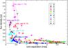 |
Fig. 6 Flux-density evolution as a function of core separation (for the inner 3 mas). In addition, the dotted line and arrows indicate the sequence of appearance of components with time and the rotational/orbital relation. For the components c, d, g, h, and i the values for βapp are given (taken from Table 1). |
Proper motion, apparent speeds of the individual jet components (based on linear regression), and estimated ejection times.
 |
Fig. 7 VLBI flux-density of the individual components and VLBI flux-density of the presumed core. |
5.5. Correlation between morphology and radio flux-density
Figure 7 exhibits the VLBI flux-density of the individual jet-features and the core component. The general flux-density of the components appears to be on a level below 0.5 Jy. The core flux-density shows three prominent peaks in 1995.05, 2003.64, and 2009.66. The core-peaks seem to be accompanied by significantly higher flux-densities of those components that appear new in the jet around these times: c in time close to the 1995.05-flare, h close to the 2003.64-flare and i close to the 2009.66-flare. All newly-appearing jet features seem to start with higher flux-densities and then appear to become fainter. This can be easily seen for i, j, k.
The single-dish radio light-curves (observed within the UMRAO program) are shown for three different frequencies (4.8, 8.0, and 14.5 GHz) in Fig. 8. Although less VLBI flux-density data are available due to less frequent sampling, the VLBI flux-density peaks of the core seem to coincide with the three peaks in the 14.5 GHz single-dish light-curve at 1995, 2004 and 2010. The source is not core dominated for about five years beginning in 1996.
We check for the pc-scale morphology at these three peak-times and find that the high flux-density values observed at 14.5 GHz coincide with significantly less jet structure of the source. The jet evolution from point-like to helical seems to be a continuous progress with time. However, at certain epochs, at times of high core-flux, the jet seems to fade or disappear. This most likely is the result of a dynamic-range effect.
The times of the high core-flux coincide with the single-dish high peaks. Two of the flux-density peaks (1995, 2010) correlate with the appearance of components, b (1995) and i (2010). These two components fit nicely into our scenario of rotation (sketched in Fig. 6). Both reveal high apparent speeds and high flux-densities. The phase of the rotation is such that these two components move along a path closer to the line of sight, with higher peak flux-densities and higher apparent velocities due to the Doppler-boosting effect.
 |
Fig. 8 Single-dish radio flux-density light-curves as obtained within the UMRAO observing program at three frequencies.The VLBI core flux-density is superimposed. |
 |
Fig. 9 From top to bottom: polarization electric vector (EVPA), degree of polarization, and total intensity flux-density single-dish data, as obtained within the UMRAO observing program at three frequencies. |
5.6. Modeling the flux-density evolution
As shown in Fig. 10, we model the long-term light-curve of 1308+326 to understand the substructure observed in Fig. 8. To this end, we divide the total light-curve into five epochs that each contain a major flare that contains sub-structures such as minor flares. The number of five divisions is arbitrary, dictated by the sampling of the light-curves and the amount of substructure visually identified within each division.
For each epoch we use a combination of four Gaussians and a constant to approximate the light-curve at each frequency. The fit is performed using a typical Levenberg-Marquardt least-squares algorithm (Marquardt 1963; Moré 1978) as implemented in the interactive data language (IDL) procedure for robutst non-linear least squares curve fitting (MPFIT; Markwardt 2009), taking into account the flux density uncertainties. The 4.8 GHz light-curve is the most sparsely-sampled and shows significant uncertainties. The best quality photometry is available for the 14.5 GHz light-curve.
In general, we find two to four outbursts per each division modeled. We can divide the observed outbursts in two types: Type A, for which a clear frequency-dependent time lag is observed; and Type B, for which all three frequencies show synchronous peaking. Type A outbursts have been associated with the emergence of bright VLBI components in the jet, and can be understood within the context of the adiabatic expansion of a plasma sphere as it propagates along the jet and away from the VLBI core. This is in agreement with our VLBI data, because these kinds of major Type A flares are preceded by the ejection of a VLBI component (e.g., component b in 1983, a in 1992, and h in 2002). Type B outbursts should reflect geometric processes that are not frequency-dependent (e.g., in 1982, 1985, and 1993), such as a precession of the jet axis or the ejection direction, and can be understood as results of Doppler boosting.
A very interesting discussion of the relation between the single dish data and the appearance of VLBI features in this source (for data at 4.8, 8, 14.5, 22, 37, and 90 GHz until 2002) can be found in Pyatunina et al. (2007). They argue that the sub-outburst between 1994 and 1995 has a different origin compared to the flares between 1988 and 1994. The former is connected with the optically thick base of the jet (where the primary perturbation occurs), and the latter was generated near the front edge of a shock associated with the propagation of the primary perturbation down the jet. This complex relationship between flux-density outbursts and the appearance of jet features deserves a more detailed analysis, and in particular a thorough investigation of the multi-wavelength data available. As discussed above, the authors favor a geometric origin of the observed effects. However, optically-thin flares with no time delay among the frequencies could also be explained by a shock-in-jet interaction with a standing re-collimation shock (e.g., Fromm 2015).
 |
Fig. 10 Top: total flux-density versus time at 4.8 (red triangles), 8.0 (blue circles), and 14.5 GHz (green squares). Solid curves show best-fit models for each frequency separately. Dashed curves show the individual Gaussian models that make up each best-fit model. Vertical dotted lines show the identified peaks of the light-curve based on the best-fit model. Gray bowties at the top of the plot mark the calculated ejection times of the VLBI components, based on our kinematic analysis. Bottom: residuals in fractional units (observed flux-density minus the best-fit model and normalized by the observed flux-density) as a function of time. Dashed lines denote the 5% level. Colors are as in the top panel. |
 |
Fig. 11 Polarization information taken from the MOJAVE webpage. We selected epochs with polarization information available close to the maxima in the single-dish flux-density light-curve. For comparison, we plot epochs close to a minimum of the light-curve. For the scale: the last image shows the inner 8mas. |
5.7. Polarization
The polarization data shown in Fig. 11 have been copied from the MOJAVE survey webpage3 and are meant to visualize the evolution with regard to the basic polarization properties. For a detailed analysis we would like to refer the reader to the webpage and the MOJAVE publications (Lister et al. 2009a, 2013). Close to or at the times of peaks in the single-dish flux-density light-curve, the total intensity jet seems to be less pronounced and less jet-structure is visible. The polarization shown in Fig. 11 shows a similar behavior whereby close to the peak of the single-dish flux-density in the radio regime, the polarization structure is less pronounced. This can be seen for all the major peaks.
 |
Fig. 12 Top (left): range of the precessing trajectory. The numbers mentioned in the legend are relative precession phases (in units of radians). Top (right): results of the fitting process of the trajectories within 0.5 mas of core-separation. Bottom (left): change of the knot trajectories beyond 0.5 mas. phi denotes for the relative precession phase of the knots. Bottom (right): fitting of the position-angle deviations is consistent with a swing period of 16.9 yr. |
A number of examples have been presented in the literature for which the observed magnetic fields in quasars tend to be parallel to the jet axis (e.g., 0735+178, 0954+658, 3C 279: Gabuzda & Cawthorne 2000) whereas the observed magnetic fields in BL Lac objects tend to be orthogonal to the jet direction (e.g., for 1803+784: Gabuzda 2000, further examples in Gabuzda & Pushkarev 2001). These orthogonal fields are likely to be indicative of an ordered helical magnetic field. For 1308+326 the magnetic field seems to be parallel to the jet axis. This again is in concordance with the classification of a quasar. However, the central region around the core shows a different orientation. Meier (2013) suggested that flat spectrum radio quasars (FSRQs) have plasma pressure dominated flows, whereas BL Lac objects have magnetic-dominated flows internally.
To investigate the polarization properties in more detail, in Fig. 9 we show the electric vector position angle (EVPA), the degree of polarization, and the total intensity flux-density single-dish data as obtained within the UMRAO observing program at three frequencies. The most prominent and intriguing property is in the evolution of the EVPA at 15 GHz (Fig. 9, top). The data before 1997 show stable plateaus in the EVPA light-curve that are indicative of preferred EVPA orientations. In the subsequent time period the total flux-density light-curve is much simpler (less structure is contained in an outburst envelope), and EVPA plateaus are not the dominant feature in the EVPA light-curve any more. The character of the variability has changed significantly. The most striking features of the EVPA light curves overall are the three apparent rotations through approximately 150 degrees. They are not equally separated in time and do not occur during a common outburst phase. All swings occur on similar timescales and in the same direction. This kind of a feature is a natural consequence of a helical magnetic field in the jet. Even without asymmetric pattern propagation, a shock moving through a straight jet pervaded by a helical magnetic field is shown to be able to produce ≲ 180° rotations of the synchrotron EVPA due to light travel times across the jet cross-section (Zhang et al. 2014, 2015). In this case, the duration of the rotation reflects the light travel time across the jet modulo Doppler boosting (Δt = Rjet(1 + z)/(δc), where δ is the Doppler factor). Alternatively, pattern propagation through a kink-like bend in a jet pervaded by a helical magnetic field yields a similar polarization-angle signature, for which the duration of the rotation is expected to be more representative of the pattern propagation time through the bend Zhang et al. (2016).
5.8. Modeling the source kinematics
As Fig. 4 shows, jet features seem to follow individual trajectories. All the trajectories differ from each other, although they do not seem to follow random paths. All trajectories can be found within a well-defined ejection cone. Feature c and a or h most likely define the cone of this beamed emission. Here we present the first results of applying a model of a precessing nozzle (e.g., Qian et al. 1991, 2009, 2014) to the data. The applied precessing nozzle model was described in detail in Qian et al. (1991, 2009, 2014) and Qian (2011). The precessing nozzle model of Qian et al. assumes that superluminal knots are ejected from a jet nozzle precessing around a fixed jet axis. The knots move independently with different bulk Lorentz factors. The precession of the nozzle leads to a swing in the position angle of the knots. The combination of a sequence of isolated knots ejected from this precessing nozzle exhibits a helical structure and the structural evolution of the whole jet as seen in our VLBA maps.
The data for five jet features within a core separation of less than 0.3–0.5 mas have been used in the calculations (c, h, i, j, k). The components a, e, f, and g have more irregular trajectory patterns and lack sufficient observational data within core separations of ~0.2–0.3 mas. Thus, their ejection position angles could not be reliably determined. Other gradients (in addition to precession, e.g., trajectory curvatures) need to be taken into account as well to explain their kinematics. Component b is at too large a distance from the core to apply the calculations to this source. Component d will be included in a new modeling attempt (Qian et al., in prep.).
The range of the precessing trajectory is shown in Fig. 12 (top, left). Figure 12 shows the results of the fitting process for two regimes: the figure at the top (right) shows the trajectories within 0.5 mas of core-separation and the figure at the bottom (left) reveals the trajectories at larger core separations. Figure 12 (bottom, right) shows that the position-angle deviations are consistent with a swing period of 16.9 yr for the precessing nozzle. The parameters for the ejection times of the components and for the precession phase are listed in Table 2. The jet features (a, b, d, e, f, g) have not been modeled. A detailed modeling and analysis is in preparation (Qian et al., in prep.).
Ejection times and precession phases for individual components modeled within the precessing nozzle model.
5.9. Estimation of the apparent half opening angle
To explore the intrinsic half-opening angle of the jet cone there is a need to derive the characteristic inclination angle (ι) of the jet of 1308+326. For this purpose we derive the apparent brightness temperature of its VLBI core, that is calculated as (Condon et al. 1982):  (1)where S (Jy) is the flux density, θ (mas) is the FWHM diameter of the circular Gaussian component, and f (GHz) is the observing frequency. Then the Doppler factor δ = [Γ(1−βjcosι)] -1 can be derived from the connection between the apparent and intrinsic brightness temperatures Tb = δTint, where βj is the intrinsic jet velocity in the units of the speed of light, and
  is the Lorentz factor. Using the equipartition temperature 5 × 10¹⁰ K as the intrinsic temperature, the median Doppler factor of the core is
  . The apparent velocity of the jet βapp (in the units of the speed of the light, c) depends on the inclination angle and the jet velocity as:
  (2)Taking into account the median Doppler factor , the maximal observed apparent velocity
  (component b) constrains the inclination angle as
  , the intrinsic jet velocity as βj = 0.998 ± 0.001, and consequently the Lorentz factor as Γ = 16.2 ± 4.4. From Fig. 12 (bottom, right) the amplitude of the initial position-angle variation of the precessing nozzle is ΔPA ~ 31.2°, that equals the apparent half-opening angle of the jet cone ψobs in the diverging part of the jet. Then using the inclination angle as , the intrinsic half-opening angle of the jet cone is
  , de-projected from the apparent cone.
5.10. Determination of the parameters of a supermassive binary black hole model for 1308+326
In the case that the injection of the jet-features into different directions within the ejection cone could be generated via a precessing origin, a binary black hole (BBH) at the center of the AGN could cause the observed phenomena. In the following, we present an explanation of the jet cone based on the presence of a BBH at the jet base. The apparent orbital period Tapp ~ 16.9 yr is derived from the precessing nozzle model presented above, and from that the rest-frame orbital period is T = Tapp/ (1 + z) ≈ 8.5 yr, where z is the redshift of the source. Using the total black hole mass estimate of Gupta et al. (2012)m ≈ 3.6 × 10⁸M⊙, which is based on optical intraday variability data, as well as the observations of the jet components described earlier, the separation to Newtonian-order between the primary and secondary black holes (BH) is r ≈ 0.014 pc. The so-called post-Newtonian parameter ε = Gm/c2/r is a suitable measure to reveal whether the dynamical friction or the gravitational radiation drives the tightening of the separation of the BBH. Using the above orbital parameters, ε ~ 0.001, which implies a BBH being in the inspiral phase of the merging process, which is when the gravitational radiation is gradually taking over the leading role in the dissipation of the binary separation.
The model assumes the jet-emitting BH perturbs the jet ejection by its orbital velocity at the launching time, giving rise to the intrinsic half-opening angle of the jet cone (Kun et al. 2014):  (3)where i indexes whether the primary BH (i = 1) or the secondary BH (i = 2) emits the jet, and κi is the angle between the Newtonian angular momentum and the ith spin. In the model this angle equals the intrinsic half-opening angle of the precessing nozzle, where it diverges. Evaluating Kepler’s third law and assuming circular orbits, the orbital velocity of the primary and secondary BH in leading order are respectively:
  Substituting i = 1 to Eq. (3), meaning that the primary BH emits the jet, the mass ratio q = m2/m1 (m1 > m2) is constrained as 0.8 < q ≤ 1, and the respective spin-angle is as κ1 ≲ 25°. Summarizing, if we assume the precessing nozzle of the jet of 1308+326 is due to the orbital velocity of the jet emitter BH, then the total mass is m ≈ 3.6 × 10⁸M⊙ from independent measurement, the rest-frame orbital period is T ≈ 8.5 yr, the separation is r ≈ 0.014 pc, and the mass ratio is 0.8 < q ≤ 1.
5.11. Limitations of a binary black hole model
Assuming circular orbits for simplicity, the separation between the two BHs in the binary model is given by:  (6)where M8 is the total mass of both BHs in units of 108M⊙, Pyr is the orbital period in years, and Rs the Schwarzschild radius of the primary, accreting BH of 108M⊙. Black hole masses of ≥108M⊙ are likely. For this kind of a small separation, the accretion disk of the primary BH is significantly disturbed by tidal effects of the secondary BH.
It is still an open question whether AGN jets are generated as disk winds via the Blandford & Payne (1982) mechanism or as BH jets via the Blandford & Znajek (1977) process. However, if the binary scenario for 1308+326 is correct, it seems unlikely that a persistent, axisymmetric jet could form from the accretion disk that is supposed to be heavily disturbed by the binary BH at radii beyond ~100 RS from the BH.
5.12. Alternative models to explain our findings for 1308+326
In the previous subsections we present first estimates for the parameters derived based on a precessing nozzle and discuss the possibility of a BBH explaining the observations. A binary supermassive BH system is not the only model that can produce precession effects in an AGN. In this subsection, we briefly mention alternative models.
Nelson & Papaloizou (2000) investigate in smoothed particle hydrodynamics (SPH) simulations how the structure of a warped accretion disk evolves with time due to the Bardeen-Petterson (Bardeen & Petterson 1975) effect produced by a maximally-rotating BH. They find that the central portions of the disc models become aligned with the equatorial plane of the BH out to a transition radius. Beyond this radius, the discs remain close to their original plane. They find that this evolution is followed by an evolution into a solid-body precession of the disc and a slow process of alignment of the outer disc with the equatorial plane of the BH.
Caproni et al. (2004) and Liu & Melia (2002) show that the misalignment between the rotation axis of the accretion disk and of the Kerr BH can explain jet precession in AGN as well. The authors successfully apply this scenario to quasars, Seyfert galaxies, and Sgr A*. However, Nixon & King (2013) show that it is unlikely for any type of BH system to explain jet precession due to the result from a combination of the Lense-Thirring effect and accretion-disc viscosity. In general, the angular momentum of the disc is not sufficiently large, in comparison with that of a spinning hole, to cause jet precession on short timescales. AGN accretion events are assumed to be uncorrelated and this would cause changes in the jet directions on comparably large timescales of ≳ 107 yr. Chaotic accretion is discussed in more detail by King & Nixon (2015) – the effect of self-gravity limits the mass of any accretion-disc feeding event. They suggest that additional disc physics is needed to explain any jet precession on timescales short compared with the accretion time.
Lubow et al. (2002) investigate the shape of a warped disc around a Kerr BH. In particular, they investigate this system under conditions such that the warp propagates in a wave-like manner. One of their results is, that in low-viscosity discs around a Kerr BH, the inner parts of the disc are not necessarily aligned with the BH. Because the shape of the inner disc depends sensitively on the radial dependence of the disc properties, a changing accretion rate can cause a change in the inner disc warp even without effecting the tilt of the outer disc. This finding contrasts with that of, for example, Nelson & Papaloizou (2000).
Lai (2003) discusses the warping of an accretion disc due to magnetically driven outflows as a possible origin for jet precession. In particular, the disk might be subject to warping instabilities and retrograde precession driven by magnetic torques associated with the outflow. The growth timescale for the disk warp and the precession period would be of order the radial infall time of the disk.
Caproni et al. (2006) study four mechanisms (tidal, irradiative, magnetic, and Bardeen-Petterson) that can cause warping and precession in galactic and extragalactic accretion disks. Eight X-ray binaries and four AGN are examined. The paper demonstrates how difficult it is to constrain the precession mechanism. The Bardeen-Petterson effect can produce the precession timescales compatible with the observed ones in all sources of their sample. However, the work by Caproni et al. (2006) shows that due to the many observational uncertainties other precession mechanisms can not easily be ruled out. In addition, more than one mechanism might be at work in a given source.
Another alternative explanation of the observed effects could result from a magnetically-arrested disc (e.g., McKinney et al. 2012; Tchekhovskoy et al. 2014). Using 3D general relativistic magnetohydrodynamic (GRMHD) simulations, Tchekhovskoy et al. (2011) show that if the magnetic flux is sufficiently high, magnetic forces impede accretion on to the BH, causing the flow to enter a magnetically arrested disk (MAD; e.g., Narayan et al. 2003). Tchekhovskoy et al. (2014) show that a precessing tilted accretion disc with a rotation axis that is misaligned with the BH spin can form shortly after a stellar disruption event in the case of the transient Swift J1644+57. In this event, a solar-mass main sequence star was disrupted by a BH of 105–106M⊙. The magnetic flux eventually became dynamically important which led to a state of MAD flow. In this MAD state, the magnetic field is, according to the authors, sufficiently strong to offset gravitational forces acting on the inner disc and to align the axis of the disc (and the jets) with the BH spin. It takes time for the entire disc and jet to align with the BH spin and during this process the jet wobbles erratically.
Jet instabilities might also produce jet precession. In particular, current-driven (CD) kink instabilities excite large-scale helical motions as shown by 3D MHD simulations for propagating jets (Nakamura & Meier 2004).
In this manuscript we describe the evolution of the jet as we deduce it from 19 yr of observations. From this, we expect that the process leading to the precession should not be of erratic nature but instead be a motion that is constant within a longer time span. The timescale of the observed long-term precessional motion thus places constraints on the potential mechanism that produces the precession. To decide which theoretical model best explains our results, detailed modeling of the data is required. We leave this to further publications and discussions.
6. Discussion
Many radio-interferometric studies of AGN reveal surprising jet properties that can not easily be reconciled within the standard scenarios. A broad spectrum of different explanations exists for the physical nature of jet components and for the launching mechanisms of jets. A similar number of model scenarios were invoked to explain curved jet structures. Based on the observations and analysis in this paper we derive and discuss the most plausible physical scenarios for the jet of 1308+326.
6.1. A swirling jet: Helical motion and precession
Several observational results that we present in this manuscript for the pc-scale jet of 1308+326 support the assumption that we see a rotating helix. The main arguments in favor of this interpretation are:
-
The pc-scale jet components are ejected in different directionswithin an ejection cone.
-
The apparent speeds of the jet components appear bundled. This can most easily be explained by a variable Doppler boosting due to a changing viewing angle.
-
The components move on different, curved paths.
-
The helical morphology appears and disappears in strong correlation with the single-dish flux and the polarized flux.
-
Changes in the direction of the pc-scale jet paths with time seem to correlate with rotations of the EVPA. The EVPA is rotating by 150 deg. This can be explained by a shock moving through a straight jet that is pervaded by a helical magnetic field.
-
The kpc-scale jet-emission changed its orientation – a changing angle to the line of sight (assuming a small and critical angle) could explain this.
Lister et al. (2013) find a period of the inner jet-position angle of 5.1 yr. However, they claim that they cannot reliably establish periodicity in any jet due to the lack of sufficient cycles in the studied MOJAVE-data and the fact that the fit for e.g., the data of 1308+326 has significant residuals.
Regarding the VLBI flux-density evolution of the individual components shown in Fig. 7 and the single-dish radio flux-density light-curves in Fig. 8, there is some relation to the approximately five year period found by Lister et al. (2013). Also, the timescale between the last two EVPA swings (Fig. 9) is roughly consistent with five years.
Another argument in favor of a helical scenario stems from the morphology of the source. The very compact structure in early times of the observations (1995) does not allow us to model a jet. Obviously the source is, or appears to be, more compact at earlier times. After several years, a jet is detectable and can be modeled. Two scenarios are possible. Either the source was compact, meaning without a jet, around 1995, or the source just appeared to be compact. It is more likely that the source only appeared to be compact and that the viewing angle must have changed. This again fits with the general impression of a helix being directed toward us.
Based on the derived kinematics for the jet features, we also find evidence for jet precession. A model of a precessing nozzle was applied to the data and is consistent with a time of 16.9 yr for a swing of the ejection angle. This model takes part of the observed feature paths into account. Further modeling of the data is in preparation (Qian et al., in prep.).
Curved jet structures are often attributed to precession effects due to binary BH merger scenarios. Our modeling reveals that, if we assume a precessing nozzle of the jet of 1308+326 due to the orbital velocity of the jet-emitting BH in a supermassive binary BH, the separation could be so small, that the accretion disk of the primary, jet-emitting BH would be significantly disturbed and the launching of a jet prevented. Stickel et al. (1993) find two large and bright galaxies, an interacting system and an apparently undisturbed elliptical galaxy, northwest of 1308+326 and a large number of faint (m≥ 20 mag) galaxies covering the whole CCD frame. Their observations were made with the 2.2 m and 3.5 m telescopes on Calar Alto, Spain, and the 2.2 m telescope on La Silla, Chile, However, according to HST observations of Pesce et al. (2002) this object appears to be truly isolated. An investigation of the applicability of a binary BH model to the data presented here is in preparation (Roland et al., in prep.).
6.2. Physical nature of jet components: Plasma following the poloidal magnetic field
Among other parameters, the magnetic field orientation seems to play a decisive role in determining the different properties of quasars and BL Lac Objects (e.g., Gabuzda 1997). A number of AGN have been studied and it was shown that the observed magnetic fields in quasars tend to be parallel to the jet axis, whereas the observed magnetic fields in BL Lac objects tend to be orthogonal to the jet direction. These orthogonal fields in BL Lac objects are likely to be indicative of an ordered helical magnetic field (e.g., Gabuzda et al. 2004). Aller et al. (1999) point out that not all BL Lacs show a preferred alignment of the magnetic field oriented perpendicular to the flow direction during relatively stable periods. The object 1308+326, although listed among the BL Lac objects, is indicated as also showing quasar type properties at times. For 1308+326 the authors report that it exhibited long-term preferred orientations that can flip between orientations parallel and perpendicular to the VLBI structural axis (Aller et al. 1999). The object1308+326 is classified as a misclassified or transition object based on the polarization properties.
For the time under investigation in this paper the magnetic field in 1308+326 seems to be parallel to the jet axis along the jet, in concordance with the classification of a quasar. However, the central region around the core appears to show a different orientation, which could hint toward a more strongly-curved magnetic field in the inner region.
6.3. Wound-up filamentary structures and helical strands
The component paths, when viewed altogether, give an impression of filaments that appear to be ordered and wound up. Similar filaments and twisted structures have been observed in a number of astrophysical contexts. To enable a comparison, we show an illustration of our results for the pc-scale jet of 1308+326 in Fig. 13. Obviously the string-like features wind-up from the inner part of the source. The structure displayed in Fig. 13 reminds us of the strings that have been observed in VLA and HST observations in the Seyfert 2 Galaxy ESO 428-G14 by Falcke et al. (1996; Fig. 14, left). Those authors describe the narrow-line region (NLR) as consisting of many individual, thin strands that seem to be very closely related to the radio jet and produce a highly complex, yet ordered, structure. They find that the jet is two-sided, with a double helix of emission-line gas apparently wrapped around the northwest side of ESO 428-G14 (0714-2914, M4-1). Falcke et al. mention that this may indicate that the emission-line strands are produced at the surface of the radio jet, possibly by an interaction of the jet with the ISM. The authors add that helical structures associated with radio jets seem to be very common because some VLBI components of quasar jets seem to move on helical trajectories (e.g., Steffen et al. 1995), and the Hα jet in NGC 4258 consists of helically twisted strands in a triple helix (Cecil et al. 1992). A schematic diagram by Cecil et al. (1992) is reproduced in Fig. 15. The magnetic field along the jet turns out to be oriented along the jet axis. An observed tilt with respect to the jet axis may also indicate a toroidal magnetic field component or a slightly helical magnetic field around the northern jet (Krause & Löhr 2004). Falcke et al. (1996) stress that the comparison with NGC 4258 is even more striking when they consider the region to the southeast, where the jet tapers off, the strands in NGC 4258 become detached from each other, they leave the helical structure, and they end up pointing in different directions. A striking similarity seems to be that the un-twisting of the strands happens in both sources at the end of the jet and is associated with strong jet bending. Falcke et al. (1996) discuss several possibile explanations for the origin for the helical strands in ESO 428-G14. One possibility is an association with strong magnetic field lines. These field lines would have to be frozen into the plasma on the surface of the jet, which is ionized by the central source. They compare these large-scale magnetic field lines with the Galactic center non-thermal filaments (Yusef-Zadeh & Morris 1987); our Fig. 14, middle. On the other hand the authors argue that interactions between the jet and the denser ISM could induce fluid-instabilities and entrainment in the jet. They refer to a discussion of the pros and cons of these models as discussed in Cecil et al. (1992). Cecil et al. (1992) argue that the emission-line velocity field of the Southeast (SE) jet in the nearby Seyfert/LINER galaxy NGC 4258 suggests that the gas moves along the helices, perhaps as a result of fluid instabilities at the interface between the jet and the interstellar medium, or of motion along magnetic flux tubes. We show the map by Falcke et al. (1996) in Fig. 14.
The image in the middle is a reproduction of the double helix nebula (Galactic center) observed at infrared wavelength with the Spitzer telescope by Morris et al. (2005). Most recently, new results for supercritical accretion disks in ultra-luminous X-ray sources and SS 433 have been published by Fabrika et al. (2015). These are based on Subaru observations of ULXs with unambiguous optical counterparts, such as single star-like objects for example Holmberg II X-1 and others. The Holmberg II dwarf galaxy as observed in HST observations reveals a similar helically wound-up object and is shown on the right in Fig. 14.
 |
Fig. 13 Schematic illustration of the region we investigate in this source, to give a better impression of the nature of components in 1308+326. This is just a rough schematic representing the scenario we propose for this source within this paper, not a depiction of component motions. With different colors we mark different origins (larger radii). |
 |
Fig. 14 From left to right: VLA and HST observations (VLA: white contour lines, HST: colored map); emission-line gas and radio plasma from helical strings in the Seyfert 2 Galaxy ESO 428-G14 (Falcke et al. 1996, for the scale: the image covers about 0.4 arcsec); the double helix nebula (Galactic center) observed at infrared wavelength of 24 μm with the MIPS camera on the Spitzer Space Telescope (Morris et al. 2005); and a multi-color optical image around the ULX “X-1” (indicated by the arrow) in the dwarf galaxy Holmberg II. The red color in the image (right) represents spectral line emissions from hydrogen atoms (courtesy of the Special Astrophysical Observatory/Hubble Space Telescope). The image size corresponds to 1100 × 900 light-years at the galaxy. |
 |
Fig. 15 Top: NGC 4258 (Ogle et al. 2014). Bottom: sketch taken from Cecil et al. (1992) showing a schematic diagram of a possible spatial structure of the triple helix SE of the nucleus in NGC 4258 (they caution the reader as to the inherent ambiguity in the identification of different segments of any given strand, especially at radii <15′′). |
What is common in these different astrophysical scenarios is the presence of wound-up filamentary structures and the relation to accretion-driven processes. In addition, an important common feature is a helically moving or wound-up object, and the explanation that the filamentary features move along magnetic field lines of magnetic flux tubes. The number of strings may be different but the general pattern is similar. In the case of 1308+326 additional motion has to be taken into account. The observations listed in Fig. 14 were taken at different frequencies and the details require a much more thorough investigation. The spatial scales of the objects displayed in Fig. 14 are somewhat different. For the Seyfert 2 Galaxy ESO 428-G14 Fig. 14 (left), the emission from the NLR is dominated by well-ordered strands of emission-line gas which are some 10 pc thick but can be more than 100 pc long. The double helix nebula in the Galactic center, Fig. 14 (middle), is at a distance of about 300 light-years from Sgr A* and about 25 parsecs in length (Morris et al. 2006). This infrared nebula, according to the authors, is most likely a torsional Alfv n wave propagating vertically away from the Galactic disk, driven by rotation of the magnetized circumnuclear gas disk. Holmberg II X-1 accretes at a high fraction of its Eddington accretion rate and possibly exceeds it (Walton et al. 2015). The observed broadband 0.3–25.0 keV luminosity inferred from their observations is LX = (8.1 ± 0.1) × 1039 erg s-1, with the majority of this flux (~90%) emitted below 10 keV (Walton et al. 2015). The triple helix SE of the nucleus in NGC 4258 (Fig. 15) of three intertwined plasma streams is 1.8 kpc long (Cecil et al. 1992) at a distance of 7.6 Mpc (Humphreys et al. 2013). Despite the differences in spatial scales and energies involved, there is a resemblance in the basic patterns which might, when investigated and understood properly, help us in the general understanding of accretion processes and jet launching.
Acknowledgments
We appreciate the very helpful advice and comments by the referee that significantly improved this paper. We thank S. Jorstad and A. Marscher for valuable comments to the draft. J. Roland contributed substantially in the discussions. This research has made use of data from the MOJAVE database that is maintained by the MOJAVE team (Lister et al. 2009b). The National Radio Astronomy Observatory is a facility of the National Science Foundation operated under cooperative agreement by Associated Universities, Inc. This research was supported in part by NASA Fermi Guest Investigator awards NNX09AU16G, NNX10AP16G, NNX11AO13G, and NNX13AP18G, and by a series of grants from the NSF, most recently AST-0607523, which made the long-term UMRAO program possible. Additional support for the operation of UMRAO was provided by the University of Michigan.
References
- Ackermann, M., Ajello, M., Allafort, A., et al. 2013, ApJS, 209, 34 [NASA ADS] [CrossRef] [Google Scholar]
- Aller, M. F., Aller, H. D., Hughes, P. A., & Latimer, G. E. 1999, ApJ, 512, 601 [NASA ADS] [CrossRef] [Google Scholar]
- Appl, S., Sol, H., & Vicente, L. 1996, A&A, 310, 419 [NASA ADS] [Google Scholar]
- Bardeen, J. M., & Petterson, J. A. 1975, ApJ, 195, L65 [NASA ADS] [CrossRef] [Google Scholar]
- Blandford, R. D., & Payne, D. G. 1982, MNRAS, 199, 883 [NASA ADS] [CrossRef] [Google Scholar]
- Blandford, R. D., & Znajek, R. L. 1977, MNRAS, 179, 433 [NASA ADS] [CrossRef] [Google Scholar]
- Böttcher, M., Baring, M. G., Liang, E. P., et al. 2015, in Extragalactic jets from every angle, Proceedings of the International Astronomical Union, IAU Symp., 313, 153 [NASA ADS] [Google Scholar]
- Bouffet, R., Charlot, P., & Lambert, S. 2012, EVN Proc., 79 [Google Scholar]
- Britzen, S., Vermeulen, R. C., Campbell, R. M., et al. 2008, A&A, 484, 119 [NASA ADS] [CrossRef] [EDP Sciences] [Google Scholar]
- Britzen, S., Kudryavtseva, N. A., Witzel, A., et al. 2010, A&A, 511, A57 [NASA ADS] [CrossRef] [EDP Sciences] [Google Scholar]
- Camenzind, M., & Krockenberger, M. 1992, A&A, 255, 59 [NASA ADS] [Google Scholar]
- Caproni, A., Mosquera Cuesta, H. J., & Abraham, Z. 2004, ApJ, 616, 99 [Google Scholar]
- Caproni, A., Livio, M., Abraham, Z., & Mosquera Cuesta, H. J. 2006, ApJ, 635, 112 [NASA ADS] [CrossRef] [Google Scholar]
- Carrasco, L., Escobedo, G., Mayya, D. Y., et al. 2012, ATel, 4234, 1 [NASA ADS] [Google Scholar]
- Cassaro, P., Stanghellini, C., Bondi, M., et al. 1999, A&AS, 139, 601 [NASA ADS] [CrossRef] [EDP Sciences] [Google Scholar]
- Cecil, G., Wilson, A. S., & Tully, R. B. 1992, ApJ, 390, 365 [NASA ADS] [CrossRef] [Google Scholar]
- Cohen, M. H., Meier, D. L., Arshakian, T. G., et al. 2015, ApJ, 803, 3 [NASA ADS] [CrossRef] [Google Scholar]
- Condon, J. J., Condon, M. A., Gisler, G., & Puschell, J. J. 1982, ApJ, 252, 102 [NASA ADS] [CrossRef] [Google Scholar]
- Doeleman, S. 2010, in Proc. 10th European VLBI Network Symposium and EVN Users Meeting, VLBI and the new generation of radio arrays, Manchester, UK, 53 [Google Scholar]
- Falcke, H., Wilson, A. S., Simpson, C., & Bower, G. A. 1996, ApJ, 470, L31 [NASA ADS] [CrossRef] [Google Scholar]
- Fromm, C. M. 2015, Astron. Nachr., 336, 447 [NASA ADS] [CrossRef] [Google Scholar]
- Gabuzda, D. C. 1997, in Relativistic Jets in AGNs, Proc. International Conference, 30 [Google Scholar]
- Gabuzda, D. C. 2000, in Astrophysical phenomena Revealed by space VLBI, Proc. VSOP Symposium, eds. H. Hirabayashi, P. G. Edwards, & D. W. Murphy (Sagamihara, Kanagawa, Japan: Institute of Space and Astronautical Science), 121 [Google Scholar]
- Gabuzda, D. C., & Cawthorne, T. V. 1992 in Variability of Blazars, Proceedings from the conference in honour of the 100th anniversary of the birth of Yriö Väisälä, eds. E. Valtaoja, & M. Valtonen (Cambridge: Cambridge University Press), 238 [Google Scholar]
- Gabuzda, D. C., & Cawthorne, T. V. 2000, MNRAS, 319, 1056 [NASA ADS] [CrossRef] [Google Scholar]
- Gabuzda, D. C., & Pushkarev, A. B. 2001, in Particles and Fields in Radio galaxies Conference, eds. R. A. Laing, & K. M. Blundell (San Francisco: ASP), ASP Conf. Proc., 250. 180 [Google Scholar]
- Gabuzda, D. C., Kollgaard, R. I., Roberts, D. H., & Wardle, J. F. C. 1993, ApJ, 410, 39 [NASA ADS] [CrossRef] [Google Scholar]
- Gabuzda, D. C., Murray, É, & Cronin, P. 2004, MNRAS, 351, 89 [Google Scholar]
- Gupta, S. P., Pandey, U. S., Singh, K., et al. 2012, New Astron., 17, 8 [NASA ADS] [CrossRef] [Google Scholar]
- Humphreys, E. M. L., Reid, M. J., Moran, J. M., et al. 2013, ApJ, 775, 13 [Google Scholar]
- Hardee, P. 2011 in Jets at all Scales, Proc. International Astronomical Union, IAU Symp., 275, 41 [Google Scholar]
- Homan, D. C., Lister, M. L., Kovalev, Y. Y., et al. 2015, ApJ, 798, 134 [Google Scholar]
- Hovatta, T., Pavlidou, V., King, O. G., et al. 2014, MNRAS, 439, 690 [NASA ADS] [CrossRef] [Google Scholar]
- Jacobs, C. S., Arias, F., Boehm, J., et al. 2014, in Proc. Reference Frames for Astrometry and Geodesy, 34 [Google Scholar]
- Jorstad, S. G., Marscher, A. P., Mattox, J. R., et al. 2001, ApJ, 556, 738 [NASA ADS] [CrossRef] [Google Scholar]
- Karouzos, M., Britzen, S., Witzel, A., Zensus, J. A., & Eckart, A. 2012, A&A, 537, A112 [NASA ADS] [CrossRef] [EDP Sciences] [Google Scholar]
- King, A., & Nixon, C. 2015, MNRAS, 453, 46 [Google Scholar]
- Krause, M., & Löhr, A. 2004, A&A, 420, 115 [NASA ADS] [CrossRef] [EDP Sciences] [Google Scholar]
- Kun, E., Gabányi, K. É., Karouzos, M., Britzen, S., & Gergely, L. Á. 2014, MNRAS, 445, 1370 [NASA ADS] [CrossRef] [Google Scholar]
- Lai, D. 2003, ApJ, 591, 119 [NASA ADS] [CrossRef] [Google Scholar]
- Liller, W., Gottlieb, E. W., & Miller, H. R. 1976, IAU Circ., 2939, 2 [NASA ADS] [Google Scholar]
- Lister, M. L., Homan, D. C., Kadler, M., et al. 2009a, ApJ, 696, 22 [Google Scholar]
- Lister, M. L., Aller, H. D., Aller, M. F., et al. 2009b, AJ, 137, 3718 [NASA ADS] [CrossRef] [Google Scholar]
- Lister, M. L., Aller, M. F., Aller, H. D., et al. 2013, AJ, 146, 120 [NASA ADS] [CrossRef] [Google Scholar]
- Lister, M. L., Aller, M. F., Aller, H. D., et al. 2016, AJ, 152, 12 [NASA ADS] [CrossRef] [Google Scholar]
- Liu, S., & Melia, F. 2002, ApJ, 573, 23 [Google Scholar]
- Lubow, S. H., Ogilvie, G. I., & Pringle, J. E. 2002, MNRAS, 337, 706 [NASA ADS] [CrossRef] [Google Scholar]
- Ma, C., Arias, E. F., Eubanks, T. M., et al. 1998, AJ, 116, 516 [NASA ADS] [CrossRef] [Google Scholar]
- Ma, C., Arias, E. F., Bianco, G., et al. 2009, Presented on behalf of the IERS/IVS Working Group, eds. A. Fey, D. Gordon, & C. S. Jacobs (Frankfurt am Main: Verlag des Bundesamts für Kartographie und Geodäsie), IERS Technical Note, 35, 1 [Google Scholar]
- Marquardt, D. 1963, An Algorithm for Least-Squares Estimation of Nonlinear Parameters, SIAM J. Appl. Math., 11, 431 [Google Scholar]
- Markwardt, C. B. 2009, Proc. Astronomical Data Analysis Software and Systems XVIII, ASP Conf. Ser., 411, 251 [NASA ADS] [Google Scholar]
- Marscher, A. P., & Gear, W. K. 1985, ApJ, 298, 114 [NASA ADS] [CrossRef] [Google Scholar]
- McKinney, J. C., Tchekhovskoy, A., & Blandford, R. D. 2012, MNRAS, 423, 3083 [NASA ADS] [CrossRef] [Google Scholar]
- Meier, D. L. 2013, in The Innermost Regions of Relativistic Jets and Their Magnetic Fields, Granada, Spain, ed. J. L. Gómez, EPJ Web Conf., 61, 01001 [Google Scholar]
- Moré, J. J. 1978, The Levenberg-Marquardt algorithm: Implementation and theory. ed. G. A. Watson, Numerical Analysis, Dundee 1977, Lect. Notes Math., 630, 105 [Google Scholar]
- Moore, R. L., Angel, J. R. P., Lebofsky, M. J., et al. 1980, ApJ, 235, 717 [NASA ADS] [CrossRef] [Google Scholar]
- Morris, M., Uchida, K., & Do, T. 2006, Nature, 440, 308 [NASA ADS] [CrossRef] [Google Scholar]
- Mufson, S. L., Wisniewski, W. Z., Pollock, J., et al. 1983, BAAS, 15, 671 [NASA ADS] [Google Scholar]
- Nakamura, M., & Meier, D. L. 2004, ApJ, 617, 123 [NASA ADS] [CrossRef] [Google Scholar]
- Narayan, R., Igumenshchev, I. V., & Abramowicz, M. A. 2003, PASJ, 55, L69 [NASA ADS] [Google Scholar]
- Nelson, R. P., & Papaloizou, J. C. B. 2000, MNRAS, 315, 570 [NASA ADS] [CrossRef] [Google Scholar]
- Nixon, C., & King, A. 2013, ApJ, 765, L7 [NASA ADS] [CrossRef] [Google Scholar]
- Ogle, P. M., Lanz, L., & Appleton, P. N. 2014, ApJ, 788, 33 [Google Scholar]
- Pesce, J. E., Urry, M., O’Dowd, M., et al. 2002, New Astron. Rev., 46, 159 [NASA ADS] [CrossRef] [Google Scholar]
- Planck Collaboration XIII. 2016, A&A, 594, A13 [NASA ADS] [CrossRef] [EDP Sciences] [Google Scholar]
- Piner, B. G., Pushkarev, A. B., Kovalev, Y. Y., et al. 2012, ApJ, 758, 84 [NASA ADS] [CrossRef] [Google Scholar]
- Pudritz, R. E., Hardcastle, M. J., & Gabuzda, D. C. 2012, Space Sci. Rev., 169, 27 [NASA ADS] [CrossRef] [Google Scholar]
- Puschell, J. J., Stein, W. A., Jones, T. W., et al. 1979, ApJ, 227, L11 [NASA ADS] [CrossRef] [Google Scholar]
- Pushkarev, A. B., Kovalev, Y. Y., Lister, M. L., & Savolainen, T. 2009, A&A, 507, L33 [NASA ADS] [CrossRef] [EDP Sciences] [Google Scholar]
- Pyatunina, T. B., Kudryavtseva, N. A., Gabudzda, D. C., et al. 2007, MNRAS, 381, 797 [NASA ADS] [CrossRef] [Google Scholar]
- Qian, S.-J. 2011, Res. Astron. Astrophys., 11, 43 [NASA ADS] [CrossRef] [Google Scholar]
- Qian, S.-J., Witzel, A., Krichbaum, T., et al. 1991, Acta Astron. Sin., 32, 369 (English translation: in Chin. Astro. Astrophys., 16, 137) [Google Scholar]
- Qian, S.-J., Witzel, A., Zensus, J. A., et al. 2009, Res. Astron. Astrophys., 9, 137 [NASA ADS] [CrossRef] [Google Scholar]
- Qian, S.-J., Britzen, S., Witzel, A., et al. 2014, Res. Astron. Astrophys., 14, 249 [NASA ADS] [CrossRef] [Google Scholar]
- Shepherd, M. C. 1997, Astronomical Data Analysis Software and Systems VI, ASP Conf. Ser., 125, 77 [NASA ADS] [Google Scholar]
- Steffen, W., Zensus, J. A., Krichbaum, T. P., Witzel, A., & Qian, S. J. 1995, A&A, 302, 335 [Google Scholar]
- Stickel, M., Padovani, P., Urry, C. M., Fried, J. W., & Kuehr, H. 1991, ApJ, 374, 431 [NASA ADS] [CrossRef] [Google Scholar]
- Stickel, M., Fried, J. W., Kuehr, H. 1993, A&AS, 98, 393 [NASA ADS] [Google Scholar]
- Tchekhovskoy, A., Metzger, B. D., Giannios, D., & Kelley, L. Z. 2014, MNRAS, 437, 2744 [NASA ADS] [CrossRef] [Google Scholar]
- Walton, D. J., Middleton, M. J., Rana, V., et al. 2015, ApJ, 806, 149 [Google Scholar]
- Watson, D., Smith, N., Hanlon, L., et al. 2000, A&A, 364, 43 [NASA ADS] [Google Scholar]
- Zhang, H., Chen, X., & Böttcher, M. 2014, ApJ, 789, 66 [NASA ADS] [CrossRef] [Google Scholar]
- Zhang, H., Chen, X., Böttcher, M., Guo, F., & Li, H. 2015, ApJ, 804, 58 [NASA ADS] [CrossRef] [Google Scholar]
- Zhang, H., Deng, W., Li, H., & Böttcher, M. 2016, ApJ, 817, 63 [NASA ADS] [CrossRef] [Google Scholar]
Appendix A: Additional data
 |
Fig. A.1 VLBA images superimposed by model-fits for 1308+326 (epoch: Jan. 1995–Jan. 1996). |


Model-fit parameters for 1308+326.
All Tables
Proper motion, apparent speeds of the individual jet components (based on linear regression), and estimated ejection times.
Ejection times and precession phases for individual components modeled within the precessing nozzle model.
All Figures
|
Fig. 1 B-array VLA image obtained at 1.46 GHz by Cassaro et al. (1999). |
| In the text | |
|
Fig. 2 Composite image of several selected VLBI images superimposed by Gaussian modelfit components. The dates of the 15 GHz observations are indicated in the plot. The core position is marked by the light blue line for better comparison. For the scale: in the last image (2008.54) the inner 6 mas are shown. We note that this is a subsample of the total of fifty observations re-modeled and re-analyzed in the paper. The complete set of images can be found in Appendix A. The contour levels shown here are listed in the following notation: lowest level (in percentage of the peak flux) and first positive level (in percentage of the peak flux), highest level (in percentage of the peak flux), and the scale factor between subsequent levels. The contour levels are: –0.6%, 76.8%, 2 (1995.05); –0.3%, 76.8%, 2 (1999.01); –0.5%, 59.3%, 1.7 (2000.06); –0.5%, 59.3%, 1.7 (2000.07); –0.3%, 52.8%, 1.6 (2000.49); –0.7%, 48.8%, 1.7 (2001.00); –0.2%, 51.2%, 2 (2001.65); –0.2%, 51.2%, 2 (2002.65); –0.2%; 51.2%, 2 (2002.90); –0.3%; 76.8%; 2 (2006.52); –0.1%, 51,2%, 2 (2008.41); –0.1%, 58.3%, 17 (2008.54). |
| In the text | |
|
Fig. 3 Distance from the core (left) and position angle as a function of distance from the core for the individual jet components (right). |
| In the text | |
|
Fig. 4 Identified components in x and y coordinates. Linear regression was performed and is shown. For more complex paths, higher order regression was calculated. To visualize the different paths we plot the inner part of the previous figure without the symbols (right), showing only the regression. To trace the rotation please follow the numbers (start at:1, end at: 8). Jet component b is not shown in this plot because data close to the core are not available to determine its path. |
| In the text | |
|
Fig. 5 Identified components in x and y coordinates. This plot shows the same relation as the plot in Fig. 4 (right), but the direction of the motion of paths in the xy-plane is indicated by arrows. The motion starts with the yellow arrow, continues to red, and ends in green. |
| In the text | |
|
Fig. 6 Flux-density evolution as a function of core separation (for the inner 3 mas). In addition, the dotted line and arrows indicate the sequence of appearance of components with time and the rotational/orbital relation. For the components c, d, g, h, and i the values for βapp are given (taken from Table 1). |
| In the text | |
|
Fig. 7 VLBI flux-density of the individual components and VLBI flux-density of the presumed core. |
| In the text | |
|
Fig. 8 Single-dish radio flux-density light-curves as obtained within the UMRAO observing program at three frequencies.The VLBI core flux-density is superimposed. |
| In the text | |
|
Fig. 9 From top to bottom: polarization electric vector (EVPA), degree of polarization, and total intensity flux-density single-dish data, as obtained within the UMRAO observing program at three frequencies. |
| In the text | |
|
Fig. 10 Top: total flux-density versus time at 4.8 (red triangles), 8.0 (blue circles), and 14.5 GHz (green squares). Solid curves show best-fit models for each frequency separately. Dashed curves show the individual Gaussian models that make up each best-fit model. Vertical dotted lines show the identified peaks of the light-curve based on the best-fit model. Gray bowties at the top of the plot mark the calculated ejection times of the VLBI components, based on our kinematic analysis. Bottom: residuals in fractional units (observed flux-density minus the best-fit model and normalized by the observed flux-density) as a function of time. Dashed lines denote the 5% level. Colors are as in the top panel. |
| In the text | |
|
Fig. 11 Polarization information taken from the MOJAVE webpage. We selected epochs with polarization information available close to the maxima in the single-dish flux-density light-curve. For comparison, we plot epochs close to a minimum of the light-curve. For the scale: the last image shows the inner 8mas. |
| In the text | |
|
Fig. 12 Top (left): range of the precessing trajectory. The numbers mentioned in the legend are relative precession phases (in units of radians). Top (right): results of the fitting process of the trajectories within 0.5 mas of core-separation. Bottom (left): change of the knot trajectories beyond 0.5 mas. phi denotes for the relative precession phase of the knots. Bottom (right): fitting of the position-angle deviations is consistent with a swing period of 16.9 yr. |
| In the text | |
|
Fig. 13 Schematic illustration of the region we investigate in this source, to give a better impression of the nature of components in 1308+326. This is just a rough schematic representing the scenario we propose for this source within this paper, not a depiction of component motions. With different colors we mark different origins (larger radii). |
| In the text | |
|
Fig. 14 From left to right: VLA and HST observations (VLA: white contour lines, HST: colored map); emission-line gas and radio plasma from helical strings in the Seyfert 2 Galaxy ESO 428-G14 (Falcke et al. 1996, for the scale: the image covers about 0.4 arcsec); the double helix nebula (Galactic center) observed at infrared wavelength of 24 μm with the MIPS camera on the Spitzer Space Telescope (Morris et al. 2005); and a multi-color optical image around the ULX “X-1” (indicated by the arrow) in the dwarf galaxy Holmberg II. The red color in the image (right) represents spectral line emissions from hydrogen atoms (courtesy of the Special Astrophysical Observatory/Hubble Space Telescope). The image size corresponds to 1100 × 900 light-years at the galaxy. |
| In the text | |
|
Fig. 15 Top: NGC 4258 (Ogle et al. 2014). Bottom: sketch taken from Cecil et al. (1992) showing a schematic diagram of a possible spatial structure of the triple helix SE of the nucleus in NGC 4258 (they caution the reader as to the inherent ambiguity in the identification of different segments of any given strand, especially at radii <15′′). |
| In the text | |
|
Fig. A.1 VLBA images superimposed by model-fits for 1308+326 (epoch: Jan. 1995–Jan. 1996). |
| In the text | |
 |
Fig. A.2 Same as Fig. A.1, but for epochs: Mar. 1996–Jul. 1996. |
| In the text | |
 |
Fig. A.8 Same as Figs. A.1–A.7, but for epochs: Sept. 2003–Apr. 2004. |
| In the text | |
 |
Fig. A.11 Same as Figs. A.1–A.10, but for epochs: Jan. 2009–Nov. 2010. |
| In the text | |
 |
Fig. A.12 Same as Figs. A.1–A.11, but for epochs: Jul. 2011–Dec. 2012. |
| In the text | |
 |
Fig. A.13 Same as Figs. A.1–A.12, but for epochs: Jun. 2013–Jan. 2014. |
| In the text | |
Current usage metrics show cumulative count of Article Views (full-text article views including HTML views, PDF and ePub downloads, according to the available data) and Abstracts Views on Vision4Press platform.
Data correspond to usage on the plateform after 2015. The current usage metrics is available 48-96 hours after online publication and is updated daily on week days.
Initial download of the metrics may take a while.