| Issue |
A&A
Volume 602, June 2017
|
|
|---|---|---|
| Article Number | A115 | |
| Number of page(s) | 25 | |
| Section | Galactic structure, stellar clusters and populations | |
| DOI | https://doi.org/10.1051/0004-6361/201629402 | |
| Published online | 26 June 2017 | |
X-ray survey of the North-America and Pelican star-forming complex (NGC 7000/IC 5070) ⋆
1 INAF–Osservatorio Astronomico di Palermo G.S. Vaiana, Piazza del Parlamento 1, 90134 Palermo, Italy
e-mail: This email address is being protected from spambots. You need JavaScript enabled to view it.
2 Harvard-Smithsonian Center for Astrophysics, 60 Garden St., Cambridge, MA 02138 USA
Received: 26 July 2016
Accepted: 20 February 2017
Abstract
Aims. We present the first extensive X-ray study of the North-America and Pelican star-forming region (NGC 7000/IC 5070), with the aim of finding and characterizing the young population of this cloud.
Methods. X-ray data from Chandra (four pointings) and XMM-Newton (seven pointings) were reduced and source detection algorithm applied to each image. We complement the X-ray data with optical and near-IR data from the IPHAS, UKIDSS, and 2MASS catalogs, and with other published optical and Spitzer IR data. More than 700 X-ray sources are detected, the majority of which have an optical or near-IR (NIR) counterpart. This allowed us to identify young stars in different stages of formation.
Results. Less than 30% of X-ray sources are identified with a previously known young star. We argue that most X-ray sources with an optical or NIR counterpart, except perhaps for a few tens at near-zero reddening, are likely candidate members of the star-forming region, on the basis of both their optical and NIR magnitudes and colors, and of X-ray properties such as spectrum hardness or flux variations. They are characterized by a wide range of extinction, and sometimes near-IR excesses, both of which prevent derivation of accurate stellar parameters. The optical color-magnitude diagram suggests ages between 1–10 Myr. The X-ray members have a very complex spatial distribution with some degree of subclustering, qualitatively similar to that of previously known members. The detailed distribution of X-ray sources relative to the objects with IR excesses identified with Spitzer is sometimes suggestive of sequential star formation, especially near the “Gulf of Mexico” region, probably triggered by the O5 star which illuminates the whole region. We confirm that around the O5 star no enhancement in the young star density is found, in agreement with previous results. Thanks to the precision and depth of the IPHAS and UKIDSS data used, we also determine the local optical-IR reddening law, and compute an updated reddening map of the entire region.
Key words: stars: pre-main sequence / X-rays: stars / ISM: individual objects: NGC 7000
Full Tables 3–5 and reduced images (FITS files) are only available at the CDS via anonymous ftp to cdsarc.u-strasbg.fr (130.79.128.5) or via http://cdsarc.u-strasbg.fr/viz-bin/qcat?J/A+A/602/A115
© ESO, 2017
1. Introduction
The star-formation region associated with the North-America (NGC 7000) and Pelican (IC 5070) Nebulae in Cygnus have received increased attention in the last decades. The two nebulae are cataloged as separate objects because of their visual appearance, but are now commonly regarded as parts of the same physical gas and dust cloud. The properties of the region were reviewed by Reipurth & Schneider (2008). The ionizing source of the nebulae has remained a mystery for decades, but was at last identified with a highly reddened O5 star (2MASS J20555125+4352246, AV ~ 9.6) by Comerón & Pasquali (2005), hidden by the dark dust cloud LDN935, lying between NGC 7000 and IC 5070. This star is remarkably isolated according to these authors: there are no other massive stars close to it, or they would have been easily detected even if highly obscured.
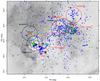 |
Fig. 1 Digital-Sky-Survey II red image of the North-America and Pelican nebulae (inverted grayscale), with overlaid the regions covered by XMM-Newton observations (big circles), and Chandra ACIS observations (squares), each labeled with its ObsId number. X-ray fields of view are drawn in red for new data, and black for archive data. ACIS-I ObsIds 13467 and 15592 share the same pointing direction and roll angle. Archive XMM ObsIds 0656780701 and 0656781201 also share the same pointing direction, but with a slightly different roll angle; only 0656780701 is labeled in the figure. Small green squares are the H58 emission-line stars; blue crosses are YSOs from RGS11. Yellow circles indicate positions and approximate sizes of the Cambrésy et al. (2002) clusters of 2MASS NIR sources. The three bigger star symbols indicate respectively the O5 star 2MASS J20555125+4352246 (cyan), the FU Ori object candidate HBC722 (=V2493 Cyg = 2MASS J20581702+4353433, green), and the FU Ori star V1057 Cyg (=2MASS J20585371+4415283, orange). |
Since the work of Herbig (1958, henceforth H58) it was known that several tens young pre-main-sequence (PMS) stars are found in this region. Welin (1973) presented also an objective-spectra study of emission-line stars in the region, and a few more young stars were studied spectroscopically by Corbally et al. (2009). Narrow-band filter studies have also revealed many emission-line star candidates (e.g., Witham et al. 2008; Armond et al. 2011), as well as many Herbig-Haro flows (Bally & Reipurth 2003; Armond et al. 2011, and also Bally et al. 2014). The strong obscuration toward many parts of the cloud undoubtedly prevents many other PMS stars to be found optically, but was no obstacle for the sensitive survey for young stellar objects (YSOs) made with the Spitzer Space Observatory (IRAC camera, Guieu et al. 2009; IRAC+MIPS, Rebull et al. 2011, henceforth RGS11). Cambrésy et al. (2002) also studied this region using 2MASS data, tracing spatial extinction variations, and finding nine clusters of near-IR (NIR) objects.
The distance of the cloud was estimated to be in the range 500–600 pc by Laugalys et al. (2006, 2007). The line of sight toward Cygnus is tangent to the corresponding spiral arm, and therefore objects at vastly different distance from the Sun can appear visually close in the sky: the Cyg OB2 association for example, only a few degrees away from NGC 7000, lies at a much larger distance ~1.5 kpc. In the direction of the North-America and Pelican (NAP), Straižys et al. (2008) find a larger-than-typical E(J−H) /E(H−K) ratio of 2.0.
The NAP region is also known to host two PMS stars in the FU Ori class: V1057 Cyg and V2493 Cyg. This latter was only known as a Classical T Tauri star (CTTS) named HBC722 before its outburst in 2010, and intensively studied thereafter (Semkov et al. 2010; Covey et al. 2011; Aspin 2011; Miller et al. 2011; Green et al. 2011; Kóspál et al. 2011, 2013; Dunham et al. 2012; Semkov et al. 2012; Liebhart et al. 2014; and Lee et al. 2015). The object V1057 Cyg was observed in X-rays (but not detected) by Skinner et al. (2007), while a positive X-ray detection of V2493 Cyg was presented by Liebhart et al. (2014). No other published X-ray study exists of this region, to our knowledge.
The strong and nonuniform obscuration toward the cloud, and its large size (~2°) are formidable difficulties when attempting to characterize the global young-star population of this star-forming region. The Spitzer RGS11 study of YSOs is extremely important in this respect, since it covers basically all the cloud, and is sensitive to even highly obscured objects. Since the selection of YSOs in RGS11 is based on the existence of non-photospheric excess IR emission from circumstellar dust (disks), it is however biased against diskless PMS stars (Class III objects in the SED-based nomenclature, or Weak-line T Tauri stars – WTTS, as opposed to CTTS – in the spectroscopic nomenclature). At typical ages of PMS stars, both CTTS and WTTS are however bright X-ray sources (with X-ray luminosities in the range log LX ~ 29−31 erg/s). Therefore, we obtained new X-ray observations at selected positions in the NAP Nebula, using both XMM-Newton and Chandra X-ray observatories, with the purpose of obtaining a more complete and unbiased census of the PMS population of this star-forming region. In addition, we analyzed here other X-ray datasets from these observatories, which were only partially examined in the published literature.
Moreover, we took advantage of two important wide-area optical and NIR surveys: IPHAS (Drew et al. 2005) and UKIDSS (Lawrence et al. 2007), covering the entire cloud, with limiting magnitudes far deeper than most other optical and NIR catalogs available in the same region.
This paper is structured as follows: Sect. 2 describes the X-ray data presented, and Sect. 3 their analysis. Section 4 describes the optical and NIR data also used in this work. Section 5 presents all results obtained. Section 6 is a discussion of the results, and Sect. 7 summarizes our conclusions.
2. X-ray observations
XMM-Newton observing log.
Chandra observing log.
The log of the X-ray observations used in this work is reported in Tables 1 and 2. We obtained three new XMM-Newton EPIC observations and two new Chandra ACIS-I observations (ACIS-I ObsIds 13647 and 15592 are in fact the same observation split in two segments, while 13648 is a distinct pointing). Four archive XMM-Newton observations were also analyzed (of which ObsIds 0656780701 and 0656781201 nearly co-pointed), as well as one ACIS-S observation: this latter has a different field of view (FOV) than the ACIS-I detector, and a slightly different sensitivity. All XMM-Newton observations, made with the EPIC camera, are composed by a set of three simultaneous observations with the PN, MOS1, and MOS2 detectors, approximately co-pointed but having different FOV shapes; PN is the most sensitive of the three, while the MOS1 (MOS2) effective area is comparable to that of ACIS-I. All XMM-Newton observations were made using the Medium filter. The Chandra ACIS images have an on-axis PSF much narrower (~0.5 arcsec) than XMM-Newton EPIC images (~4 arcsec): this implies not only a better spatial resolving power, but also that less counts are needed for a significant source detection (~4 X-ray counts vs. ~40 for the PN+MOS combination) because the background contribution in the EPIC images is usually non-negligible, while it is in ACIS images. Far from optical axis, the PSF degrades sensibly in ACIS images, while that of XMM-Newton images is rather uniform across the FOV.
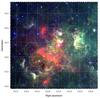 |
Fig. 2 True-color WISE image of the region. Red: 22μ, green: 12μ, and blue: 4.6μ channels, respectively. The big circles and squares indicate the X-ray FOVs as in Fig. 1. North is up and east to the left. At a distance of 560 pc, the 3-degree sky region shown measures 29.3 pc on a side. |
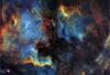 |
Fig. 3 Optical emission-line image of part of the region (courtesy Ondřej Podlucký, http://astrofotky.cz), in the lines of [O III] (blue), Hα (green) and [S II] (red), showing increasing ionization toward a location behind the obscuring dust. The white arrow indicates north. |
We tried to optimize our X-ray pointings, guided by the large-scale distribution and local spatial density of YSOs from Guieu et al. (2009). Therefore, we chose ACIS-I where the YSO density was highest, but preferred XMM-Newton with its larger FOV for the sparser regions. Figure 1 shows a Digital-Sky-Survey (DSS) red image of the region, with indicated all the X-ray observations studied here, and also the RGS11 YSOs, and H58 PMS stars; the illuminating O5 star, and the two FU Ori objects are also indicated, as well as the NIR clusters found by Cambrésy et al. (2002). The sub-regions with the highest YSO density are the Gulf of Mexico, covered by our ACIS field 13648, and the “Pelican”, covered by our ACIS fields 13647 and 15592. The less-obscured part of the cloud containing V1057 Cyg, covered by XMM-Newton archive ObsId 0302640201, contains only few YSOs.
Besides the studies mentioned above, more evidences can be presented in favour of the North-America and Pelican Nebulae being part of the same cloud; this is especially important in this part of the sky because of the mentioned tangent-arm geometry, and in this particular nebula to ascertain that the foreground obscuring cloud is physically associated with the bright nebulae and is not much closer along the line of sight. For example, the WISE (Wright et al. 2010) images in four NIR bands at 3.4, 4.6, 12, and 22μ demostrate the presence of dense, hot dust behind the dark nebula LDN935 (Fig. 2), with a geometry approximately centered on the illuminating O5 star. The distance of the dark cloud from us is therefore the same as the distance of the bright nebulae oscured by it. The region with the highest YSO density, just southeast of the O5 star and inside our ACIS 13648 field, is also seen in the WISE image to be one of highest obscuration.
The same qualitative conclusion that the North-America and Pelican Nebulae are the same physical cloud is reached by inspecting an optical emission-line image, obtained using narrow-band filters centered at the [O III], Hα, and [S II] optical lines, shown in Fig. 3. The ionization (highest for [O III]) has a global pattern, centered close to the O5 star; there is no other obvious ionization center, based on the optical-line image.
All X-ray images studied here are shown in Figs. 4–6. In these true-color images, the red (green, blue) intensity is proportional to detected X-ray counts in the soft (medium, hard) X-ray band. Blue sources are typically highly absorbed objects, with a strong low-energy cutoff in their X-ray spectrum. The Chandra FOVs are indicated, as well as the O5 star and the FU Ori objects.
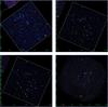 |
Fig. 4 True-color X-ray images of individual observations, slightly smoothed to emphasize point sources. Red: 0.4–1.2 keV; green: 1.2–2.4 keV; blue: 2.4–7.9 keV. Panel a), upper left: ACIS-I ObsId 13648 (in the Gulf of Mexico). The ACIS-I FOV size is 16.9 arcmin on a side. b), upper right: ACIS-I ObsId 13647 (“Pelican”). c), lower left: ACIS-I ObsId 15592, with same pointing as ObsId 13647 (panel b)). Comparison with this latter ObsId makes source variability very evident. d), lower right: XMM-Newton ObsId 0679580101 (“Pelican hat”). In all XMM-Newton images shown here, MOS1, 2 and PN data are combined together. |
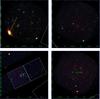 |
Fig. 5 X-ray images as in Fig. 4. Panel a), upper left: XMM-Newton ObsId 0679580201. The brightest source (2XMM J205347.0+442301) (classified as a star by Lin et al. 2012) produces both diffraction spikes and a stripe of out-of-time events, accumulated during CCD readout. The white line outlines the eastern part of ACIS ObsId 13647 FOV. b), upper right: XMM-Newton ObsId 0679580301, toward the highly obscured region LDN 935. The plus sign labeled “O5” is the O star 2MASS J20555125+4352246 from Comerón & Pasquali (2005). c), lower left: archive ACIS-S ObsId 14545. The two white squares indicate ACIS-S chips 6 (front-illuminated, right) and 7 (back-illuminated, left), which have different sensitivities and are analyzed separately. This ObsId also has data from chips 2, 3, and 8, shown in the same figure; however the sensitivity and spatial resolution of these chips is inferior, and they are not considered further here. Near the center of the image, the green plus sign indicates the new FU Ori candidate HBC 722. To the SW a part of ACIS 13648 FOV can be seen. d), lower right: Archive XMM-Newton ObsId 0302640201, just north of ACIS-S ObsId 14545 (seen in lower-right corner). Near image center the FU Ori star V1057 Cyg is labeled. |
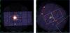 |
Fig. 6 X-ray images as in Fig. 4. Panel a), left: Archive XMM-Newton ObsId 0556050101, overlapping XMM ObsId 0679580201 of Fig. 5, panel a). The bright source is the same as in that figure. The distribution of background emission seen here is caused by the small-window mode used here for the MOS cameras (not for the PN camera). b), right: archive XMM-Newton ObsId 0656780701+0656781201. The slight pointing difference between the two ObsIds causes the inter-chip gap pattern seen in the figure. The image overlaps completely with the ACIS 14545 FOV, and partially with ACIS 13648 FOV in the lower right corner. The tight group of X-ray sources surrounding HBC 722 (Fig. 5, panel c)) is unresolved here. |
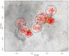 |
Fig. 7 Same field and background image as in Fig. 1, with small symbols now indicating: X-ray detected sources (red crosses), near-IR excess objects (orange triangles), and Hα-excess objects (dark-red circles). Big circles and squares are X-ray FOVs as in Fig. 1. |
3. X-ray data analysis
The X-ray datasets were processed using standard software packages (CIAO v4.8 for Chandra and SAS v11 for XMM-Newton data), and exposure maps at a representative energy of 1 keV were computed using the same packages. Source detection was made using PWDetect (v1.3.2) for Chandra data, and its XMM-Newton analog PWXDetect (Damiani et al. 1997a,b). The front- and back-illuminated chips of ACIS-S ObsId 14545 were analyzed separately. ACIS-I ObsIds 13647 and 15592, sharing the same pointing direction and roll angle, were only analyzed jointly. This was also the case for archive XMM ObsIds 0656780701 and 0656781201. Spurious detections associated with diffraction spikes or out-of-time events (Fig. 5, panel a; Fig. 6, panel a) were manually eliminated. We then merged all individual X-ray detection lists according to computed position errors, separately for XMM-Newton and Chandra, giving priority to highest-significance detections. Thus, each detected X-ray source received its IAU-recommended instrument-specific designation. The match and merging of XMM-Newton and Chandra detection lists was made in a subsequent step, taking in mind the much better spatial resolution of this latter, and therefore giving priority to the Chandra source positions and properties in ambiguous cases (see, e.g., the tight group of sources near HBC 722 in Fig. 5, panel c, which is unresolved by XMM-Newton in Fig. 6, panel b). The final X-ray source list comprises 721 objects, of which 378 ACIS detections (of which 34 with an XMM-Newton counterpart), and 343 XMM-Newton-only detections. The chosen detection threshold, corresponding to approximately one spurious detection per field, ensures that no more than approximately ten of the 721 detections are spurious. The positions of all X-ray detections are shown in Fig. 7.
4. Auxiliary data: optical and near-IR
We complemented the X-ray data with data taken from the IPHAS DR2 (Barentsen et al. 2014), 2MASS PSC, and UKIDSS DR10plus GPS (Lawrence et al. 2007; table “reliableGpsPointSource”). All of these surveys cover the entire spatial region considered here. We extracted sources from a region of radius 1.5° centered on (RA,Dec) = (313.7,44.4). This yielded 1117062 IPHAS sources, however after applying the recommended screening (keeping only sources with flags a10 = 1 and a10point = 1, i.e. point-like sources with high signal-to-noise ratio in all bands) their number reduces to 161635 sources.
Detected X-ray sources in the NAP.
The screened 2MASS PSC source list (flag ph_qual different from E, F, U, X, flag cc_flg different from p, d, s) contains 339774 sources. The UKIDSS source list instead contains 980770 sources. This is much larger than the number of 2MASS sources because of the greater depth of the UKIDSS survey; however, the UKIDSS data do not supersede the 2MASS data, since they saturate at the bright end (J ≤ 12), where 2MASS still contains reliable data. We therefore use both sets of data, after an examination of their agreement on the sources common to both (see Appendix A). For these latter, the photometric errors are much lower in the UKIDSS than in the 2MASS magnitudes, so we adopted the UKIDSS ones whenever available. At large reddening, often found in this region, the UKIDSS photometry differs from 2MASS, so a slight recalibration was applied to agree with the 2MASS system (Appendix A).
Optical/NIR photometry for X-ray sources.
We matched each of these source catalogs with our X-ray source list, up to a maximum offset of 4σ, where σ is the combined positional error from our X-ray detection code, from the 2MASS PSC error err_maj, or set fixed to 0.07′′ for the IPHAS and UKIDSS sources. There are 568 2MASS, 235 IPHAS, and 300 UKIDSS counterparts to our X-ray sources.The number of total counterparts using the combined NIR catalog is instead 548, lower than the 2MASS counterparts alone because of incomplete sets of magnitudes for several stars.115 X-ray sources remained unidentified. The number of spurious matches between X-ray and optical (and NIR) sources is difficult to evaluate, since assumptions usually made to compute it (uniform spatial distributions of the two matched sets) are not fulfilled here. As we have seen above, X-ray sources are found near regions of strong obscuration, where the optical and NIR source density is much smaller than average, and changes on very small spatial scales. Moreover, the PSF (and source position error) of the XMM-Newton data is much larger than that of the Chandra ACIS data, so that even if the optical and NIR spatial density were uniform there is a higher chance of spurious matches for XMM-Newton X-ray sources than for the Chandra ACIS sources.
Finally, we positionally matched our X-ray source list with the YSOs from RGS11, obtaining 184 matches out of all 802 YSOs falling in our X-ray FOVs (by class: 33/189 for flat-spectrum YSOs, 23/195 for Class I, 123/370 for Class II, 4/23 for Class III, and 1/25 for unclassified YSOs). Of the H58 stars, 45 were falling in the X-ray FOVs and 31 were X-ray detected. It is worth remarking that the ACIS fields yielded larger detection percentages than the XMM-Newton fields, whose higher background resulted in a lower sensitivity. The median threshold X-ray luminosity for ACIS detection was found to be log LX ~ 29.9 erg/s, while the corresponding value for XMM-Newton is log LX ~ 30.4 erg/s, at the average absorption values inferred for these YSOs (see below). Considering all ACIS FOVs, 115 YSOs were detected out of 373 observed (by class: 25/94 flat-spectrum, 17/118 Class I, 72/132 Class II, and 1/8 Class III). The corresponding numbers for the XMM-Newton FOVs are 83 detections out of 551 observed YSOs (by class: 11/136 flat-spectrum, 10/115 Class I, 58/274 Class II, and 3/17 Class III).
Our X-ray source properties and identifications are reported in Tables 3 and 4.
5. Results
5.1. Distance
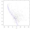 |
Fig. 8 An (i,r−i) CMD of stars toward two heavy-obscuration regions in LDN 935, with a 10-Gyr isochrone from BHAC at zero reddening and distance of 560 pc (bluesolid curve).Blue dashed curves correspond to distances smaller and larger by 20%, respectively. Only datapoints with errors <0.05 on both i and r−i are shown. |
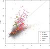 |
Fig. 9 IPHAS (r−Hα,r−i) diagram. The grayscale background is a 2D histogram of all IPHAS objects in the sky region of Fig. 1, with bin sizes of 0.01 in both axes. The dashed line is the CTTS-star limit. Symbols as in Fig. 7, with the addition of YSOs from RGS11 (violet squares), and emission-line stars from H58 (dark-green squares). Hundreds of faint stars above the dashed line are not selected here as Hα-emission stars because of their position in the CMD. |
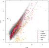 |
Fig. 10 Near-IR color-color diagram (J−H,H−K), using both 2MASS and UKIDSS data. Symbols as in Fig. 9. The arrow indicates the reddening vector corresponding to AV = 1. The dashed line is the adopted limit to select NIR-excess objects from this diagram. The blue lines in the lower-left part are unreddened BHAC isochrones for ages of 1, 3, 10, 30, 100 Myr, and 10 Gyr, and masses between 0.08−1.4 M⊙. BHAC evolutionary tracks for masses of 0.1, 0.3, and 0.5 M⊙ are shown in green.In this and following color-color diagrams, only data with errors less than 0.1 mag on each color are shown. |
The deep IPHAS photometry enabled us to perform a new determination of distance, relying upon the assumption that the obscuring dark cloud LDN935 lies immediately before the star-forming region, as argued above. The method (already used by Prisinzano et al. 2005, to determine the distance of the young cluster NGC 6530) fits the lower envelope of datapoints in the color-magnitude diagram (CMD) to the shape of the main sequence of field stars, which are the lowest-luminosity field stars at each given color. It is therefore independent of any assumption on the cluster age or specific isochrone set. To apply the test we selected two heavily obscured regions in LDN 935 (12-arcmin radius circles around (RA,Dec) = (314.2,43.6) and (312.9,44.9), respectively), whose CMD using IPHAS data is shown in Fig. 8. Also shown is a 10-Gyr isochrone from Baraffe et al. (2015; henceforth BHAC) at zero reddening and distance of 560 pc, which provides a good fit to the lower envelope of datapoints(solid), at least for r−i < 1. The dashed curves (±20% in distance) moreover suggest that the distance is unlikely to be larger than ~650 pc. Therefore, the new data are in good agreement with the accepted distance of the complex (560–600 pc, Laugalys et al. 2006, 2007). Since the BHAC tracks are not currently available for the IPHAS filter set we have recalibrated them for this filter set starting from those for the Johnson/Cousins filters, as explained in Appendix B.
5.2. Hα-emission stars
The IPHAS survey also provides a r−Hα index, useful to select Hα-emission objects over wide sky areas. A r−Hα vs. r−i diagram for NAP is shown in Fig. 9. Datapoints in the upper part of the diagram are emission-line stars. In particular, we show with a dashed line the color-dependent limit used by Kalari et al. (2015) to select CTTS stars. Almost all of the H58 PMS stars, and most of the RGS11 YSOs fall above that limit. We therefore selected all stars significantly above that line (4σ above errors) as candidate CTTS. However, this choice yielded hundreds objects falling too low in the optical CMD (i > 18, r−i ~ 1, much below the ZAMS at the NAP distance), and mostly in the northeast quadrant of the surveyed region, that is, spatially far from the known YSOs, that are thus unlikely to be young stars in the NAP. These are probably unrelated emission-line stars at much larger distances, and are therefore not included in our emission-star list, which comprises 153 stars (of which 30 detected in X-rays). The spatial distribution of accepted emission-line stars selected from the r−Hα index is shown in Fig. 7.
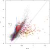 |
Fig. 11 Optical-IR color-color diagram (r−i,H−K). Symbols as in Figs. 9 and 10. The dashed line is the adopted limit for selection of NIR-excess objects from this particular diagram. The magenta thick line in the lower-left part indicates the location of unreddened stars in the mass range 1−1.4 M⊙. Much larger fractions of the H58 stars and of the RGS11 YSOs show a NIR excess using this diagram, compared to that of Fig. 10. |
5.3. Optical and near-IR color-color diagrams
Different color-color diagrams can be used to estimate the amount of reddening and the possible presence of non-photospheric color excesses, likely originated in circumstellar dusty disks. The (J−H,H−K) diagram for the entire NAP region is shown in Fig. 10. In agreement with Straižys et al. (2008), we find that the Rieke & Lebofsky (1985) reddening-vector slope does not adequately describe the slope of datapoints in this diagram; therefore, we devote Appendix C to the careful determination of the reddening vector slopes for all independent color pairs in the NAP optical-NIR catalog. This redetermined reddening vector is shown in Fig. 10 and in all following color-color diagrams. To the right of the main locus of reddened normal photospheres, stars with K-band excess emission are found. We set a fiducial limit to define such stars as the dashed line in the figure. Stars significantly (>4σ) to the right of this line were selected as NIR-excess objects, or candidate CTTSs (orange triangles in the figure). The complete list of NIR-excess objects includes stars selected from other optical-NIR color-color diagrams (see below), hence the presence of several of them also to the left of the fiducial limit in Fig. 10. It should be remarked that this diagram, although widely used, is not a very efficient tool to select CTTSs: none of the CTTSs found by H58 (green squares) falls to the right of the limiting line in this diagram. Also very few of the RGS11 YSOs are found in the CTTS region of the diagram.
We have studied the properties of several mixed optical-NIR diagrams in the young cluster NGC 6530 (Damiani et al. 2006), which enable the selection of many more NIR-excess stars than the (J−H,H−K) diagram. Therefore, we used similar mixed optical-NIR diagrams also for the NAP stars. Figure 11 is a (r−i,H−K) diagram, where we again have drawn a fiducial line (with the slope of the reddening vector, see Appendix C), sufficiently distant from the bulk of stars, separating normal reddened photospheres (to its left) from NIR-excess stars, whose NIR colors are too red compared to the respective r−i colors for any reddening value. The usefulness of this diagram is immediately seen by considering that here most of the H58 CTTSs and of the optically detected RGS11 YSOs are found to the right of our fiducial limit, together with other tens NIR-excess stars (orange triangles) not present in previously-known catalogs. The bulk of normal field stars are instead found along a reddened-photosphere locus, well reproduced by the available BHAC models (blue lines) and reddening vector. The magenta segment of the BHAC isochrones represents the locus of (unreddened) stars with M> 1 M⊙; the upper envelope of datapoints is instead populated by the lowest-mass dwarf stars (isochrones are shown down to a minimum mass M = 0.08 M⊙). Most of the X-ray sources in the NAP region do not show NIR excesses, neither from Fig. 11 nor from Fig. 10. Some of them follow well the zero-reddening isochrones, down to the substellar-mass limit, while in general Figs. 10 and 11 suggest that they are characterized by a wide range of reddening. The same conclusion was reached in Sect. 2 above from the visual inspection of the true-color X-ray images of Figs. 4–6.
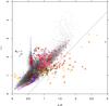 |
Fig. 12 Optical-IR color-color diagram (r−i,J−H). Symbols as in Figs. 9 and 10. The dashed line is the adopted limit for selection of NIR-excess objects from this particular diagram. |
Another useful diagram is r−i vs. J−H (Fig. 12) although in this case the number of NIR-excess stars selected is smaller than from Fig. 11. However, this color combination enables us to identify the lowest-mass stars more securely than previous diagrams, as it breaks the near-degeneracy between intrinsic stellar color and reddening, for masses below ~0.3 M⊙ (green curves in Fig. 12 are BHAC evolutionary tracks for the lowest masses), as long as a star has photospheric colors. An even more detailed, non-degenerate determination of mass and reddening for individual stars is made possible by the rarely-used, but very interesting, (r−i,i−H) diagram shown in Fig. 13. The high-precision IPHAS and UKIDSS photometry undoubtedly are a major ingredient for this representation being so useful. Dwarf M stars, with M ≤ 0.5 M⊙, stand out clearly above the main locus of more massive stars, and are therefore effectively selected using this diagram. Most of them are unreddened (2 < i−H < 3), of which 34 detected in X-rays. This diagram indicates that the majority of X-ray sources having an optical counterpart have instead larger reddening, in the range AV ~ 2−4. Only 3–4 of the H58 CTTSs have inferred masses M ≤ 0.5 M⊙, while all others are more massive (if their i−H color is photospheric, which may not be strictly true, see Fig. 11). The few X-ray sources to the left of the unreddened isochrones are not easily justified by any current model: their discrepant colors might arise from spurious matches between the IPHAS and 2MASS+UKIDSS catalogs, or from variability in the optical or NIR bands.
We estimated the number of foreground X-ray sources as in Pillitteri et al. (2013), by integrating the field-star X-ray luminosity function (Favata & Micela 2003) up to the NAP distance, and down to the limiting X-ray flux values appropriate to our X-ray observations (see Sect. 5.8 and Fig. 28). We estimate that about 67 foreground sources are detected cumulatively in all XMM pointings, and 18 in all ACIS pointings, for a total of ~85 foreground sources not related to the NAP. Being older than the NAP members, these are expected to be found among the softest detected X-ray sources (Güdel et al. 1997). The unreddened M stars found above, and many other X-ray sources found along the unreddened sequence in the diagram of Fig. 13, are therefore the best candidates as foreground sources.
The number of NIR-excess stars is 208 (of which 29 detected in X-rays, and 38 common to the Hα-excess list), and their spatial distribution can be seen in Fig. 7, with the maximum density found in the Pelican region.The 273 X-ray undetected NIR-excess and Hα-excess stars are listed in Table 5.
Optical and NIR photometry for X-ray undetected stars with IR or Hα excess.
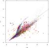 |
Fig. 13 Optical-IR color-color diagram (r−i,i−H). Symbols as in Figs. 9 and 10. Stars less massive than 0.5 M⊙ (M-type) fall above the dashed line. |
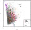 |
Fig. 14 Optical color-magnitude diagram (i,r−i). Symbols as in Figs. 9 and 10. Unreddened BHAC evolutionary tracks are here shown for masses of 0.1, 0.2, 0.3, 0.5, 0.7 M⊙ (green), and 1 M⊙ (magenta).In this and following color-magnitude diagrams, only data with errors less than 0.1 mag on each axis are shown. |
5.4. Color-magnitude diagrams
Figure 14 is an optical CMD for the whole NAP region. Comparison with Fig. 8 shows that thousands background stars are observed behind the cloud. Since no reddening correction was applied here, the apparent masses of, for example, the H58 stars, which as seen above are reddened by several magnitudes in the V band, are much lower than their actual values; these are in most cases larger than 0.5 M⊙ as discussed above. The few tens X-ray sources and NIR-excess stars below the 10-Gyr isochrone are not necessarily lying at larger distances: in fact, they share the same position in this CMD as many of the RGS11 YSOs. Below-ZAMS NIR-excess objects were already found in other young clusters like NGC 6530 (Damiani et al. 2006) or NGC 6611 (Guarcello et al. 2010), and may be attributed to photospheres obscured by edge-on disks, seen only in scattered light.Since datapoints shown in Fig. 14 have all errors less than 0.1 mag, attributing their position in the CMD to errors seems instead unlikely.
Considering X-ray sources, there is no clear sequence or cluster locus in the CMD, probably because of the large scatter in extinction from star to star. Estimating individual extinction values is subject to large uncertainties, as we will discuss in the following. Two-thirds of X-ray sources lack an IPHAS counterpart, probably because they are too highly reddened. Figure 15 shows therefore the NIR CMD (J,J−H). The frequency and intensity of non-photosperic dust emission in these NIR bands is probably lower than in the K band, from the comparison of Figs. 11 and 12. The distribution of datapoints, elongated parallel to the reddening vector, suggests that indeed reddening, rather than H-band excess, is responsible for most of the spread toward red colors, by up to AV ~ 35 for the most reddened X-ray sources and YSOs with a NIR counterpart. A considerable number of X-ray sources has inferred AV ≥ 10, if indeed their J−H color is photospheric.
Finally, Fig. 16 shows the (H,H−K) diagram. The spread toward red colors is here probably due to a combination of reddening and K-band excess emission. The diagram shows that several tens new NIR-excess sources (not identified with a YSO from RGS11) are much fainter objects (with H> 15) than these latter. The majority of X-ray sources has H−K ≤ 0.5, no NIR excesses, and H magnitudes fainter than the H58 stars.
In the presence of strong differential reddening, as we discuss below, incompleteness affects the optical CMD much more than the NIR CMD: from Fig. 14 we see that while for low reddening the IPHAS photometry reaches down to the sub-stellar limit at the NAP distance and ages ≤ 3 Myr, the mass completeness limit rises rapidly for increasing extinction (e.g., ~1 M⊙ for AV ~ 5). Our combined NIR catalog reaches at least 3–4 mag deeper than the substellar limit at the same age, and is moreover much less sensitive to extinction (Figs. 15 and 16), which accounts for the much larger number of NIR counterparts to X-ray sources (548) compared to optical counterparts (235).
5.5. Extinction and reddening
The wide range of extinction indicated by the above diagrams may have a local component, arising in the individual circumstellar environments, but also shows definite large-scale patterns, as shown by Cambrésy et al. (2002) using 2MASS data. Here we take advantage of the more precise UKIDSS NIR data to build a more detailed extinction map of the NAP, based on the average J−H color, as shown in Fig. 17. Optical extinction is approximately ten times the average J−H (minus 0.5), so that the most obscured regions correspond to AV ~ 35, and the “green” regions in the map correspond to AV ~ 15.
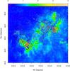 |
Fig. 17 Spatial map of average J−H (scale at figure top) as a measure of extinction. Indicated are the X-ray FOVs as in Fig. 1. The datapoints indicate X-ray sources (red) and RGS11 YSOs (orange). |
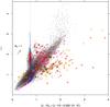 |
Fig. 18 Mixed color-color diagram of r−i vs. corrected color (J−H)c (see text). Symbols as in Figs. 9 and 10. The vertical dotted line indicates the value (J−H)c = 0.75. |
The J−H color may be considered as the best indicator of reddening for our NAP candidate PMS members, either X-ray detected or from Hα- or NIR excess: it is available for most candidate members (548/721 X-ray sources, 817/994 X-ray+Hα+NIR-excess sources), is less affected by non-photospheric emission than the K band magnitudes, and normal stars fall within a small J−H color range (Fig. 12), especially for M< 1 M⊙. The mass dependence of J−H color may moreover be partially compensated by using a “corrected” color, of the form:  (1)for stars not classified as NIR-excess sources; the intrinsic unreddened value of (J−H)c is ~0.75 for all masses in the range 0.08−1 M⊙, and ages ≥ 20 Myr, with slight deviations for younger low-mass stars (Fig. 18). Individual visual extinction AV, for stars with (J−H)c> 0.75, can be estimated therefore as
  (2)where the last factor above is the (constant) reddening vector slope, equal to 7.318 (using the Rieke & Lebofsky 1985, reddening law). For stars more massive than 1 M⊙ this underestimates AV, since their intrinsic (J−H)c color is lower (bluer) than 0.75. Extinction AV for stars with a NIR excess is instead estimated from the J−H color alone (this is again an underestimate for M> 1 M⊙).
By using these individual AV values (converted to the IPHAS bands Ai and E(r−i) as explained in Appendix C) we have built the dereddened optical CMD, shown in Fig. 19. The clustering of X-ray sources at (r−i)0 ~ 1 is probably an artifact resulting from our underestimated reddening for stars above 1M⊙. The bulk of X-ray sources, if lying at the NAP distance, are found in a 2-mag wide strip corresponding to the PMS band, between ages 1–10 Myr, also populated by the majority of H58 stars (on average brighter than the rest of the X-ray-source counterparts) and optically-visible YSOs. Tens of NIR-excess stars are found apparently below the main sequence at the Nebula distance, as remarked above. The unreddened X-ray-detected M stars selected from Fig. 13 have especially reliable positions in this diagram, since they required no dereddening: they do not form a proper sequence in this CMD, but are mixed to other low-mass NAP X-ray sources. They might still be foreground, active M dwarfs, three to ten times closer than the NAP; this diagram does not permit to confirm (nor exclude) their NAP membership.
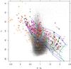 |
Fig. 19 De-reddened optical CMD. Symbols, isochrones and evolutionary tracks as in Fig. 14. The black plus signs are the unreddened M stars from Fig. 13 (with 2 < (i−H) < 3). |
5.6. Spatial distributions
As found for example by Cambrésy et al. (2002) and RGS11, the spatial distribution of young stars in the NAP is highly non-uniform. This non-uniformity also holds for the X-ray source distribution (Figs. 4 to 6). Therefore, we examine here in more detail the properties of each spatial sub-region. The individual panels of Figs. 20 and 21 permit a comparison between the spatial distributions of all sets of data considered here. The background grayscale image represents the local density of all optical and NIR objects (in white the lowest densities), which is inversely correlated with the mean reddening (Cambrésy et al. 2002) shown in Fig. 17, but is a somewhat more versatile indicator (e.g., for sources with too noisy or missing J magnitudes). As in Figs. 1 and 7, big solid circles and squares are X-ray FOVs, while RGS11 YSOs are indicated with black plus signs. X-ray sources are here instead color-coded, according to their observed J−H color, with the color scale shown in the upper left panel of Fig. 20. X-ray sources without a NIR counterpart, or with missing J−H, are drawn with a red color, assuming that high extinction is the reason for the missing measurement.
The “Pelican hat”, as in RGS11, is the northernmost field in our survey (Fig. 20, top left), covered by XMM-Newton ObsId 0679580101. The region hosts a local concentration of YSOs (see RGS11), nearly coincident with a region of enhanced obscuration, elongated along N-S direction, through the center of the XMM-Newton FOV. Curiously, most X-ray detected sources in this field lie to the right of center (inside the dashed rectangle in the figure). Their J−H colors suggest they are an inhomogeneous group, either with very different extinction values, or a wide range of masses (or both). Very few of these in-rectangle X-ray sources also possess a NIR excess. At the same time, they are not spread uniformly across the X-ray FOV, as if they were an unrelated field-star population1, but closer to the West side of the obscured region. Therefore, these X-ray sources appear to correspond to a sub-population of the NAP which is missed by YSO and CTTS searches, even using Spitzer or mixed optical-IR criteria; they also lack strong Hα emission, as are not coincident with IPHAS-selected CTTSs. The properties of this group of X-ray sources are perhaps best interpreted as a group of relatively older WTTS members of the NAP population, and their spatial placement relative to the younger YSOs (and the currently cloud overdensity seen from the star-count map) as an indication of sequential star-formation episodes, proceeding from west to east in this particular region of the NAP.
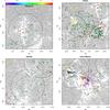 |
Fig. 20 Comparison between spatial distributions of X-ray sources, YSOs and other young stars in each X-ray FOV. The background grayscale image is a 2D histogram of the combined optical-NIR object density, showing clearly high-obscuration regions. Solid black circles and squares are XMM and ACIS FOVs, respectively. Symbols as in Figs. 9 and 10, except that here X-ray sources (crosses) are color-coded according to their J−H color (with the color scale show in the top left panel). X-ray sources without a NIR counterpart are shown in red. Black plus signs indicate positions of all RGS11 YSOs, regardless of their identification with X-ray or other cataloged objects. Small empty circles are young stars from Armond et al. (2011; black) and Welin (1973; violet). Yellow circles are 2MASS star clusters from Cambrésy et al. (2002). The black dashed rectangular regions are defined here as places with a local overdensity of X-ray sources, not matched by an overdensity of YSOs. The three bigger star symbols indicate respectively the O5 star 2MASS J20555125+4352246 (cyan), and FUOrs HBC722 (green) and V1057 Cyg (orange). |
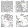 |
Fig. 21 Continuation of Fig. 20. In the lower-right panel the zooming factor is much larger than in the other panels, to help visually resolve the dense cluster in the center. The 2D bin size of the background image (and the density-grayscale conversion) is the same in all panels here and in Fig. 20. |
The upper-right panel of Fig. 20 (Pelican field proper) was covered by one new (0679580201) and one archival (0556050101) XMM-Newton observations, and by Chandra ACIS-I ObsIds 13647 and 15592; it hosts most of the H58 stars, and a large number of RGS11 YSOs (though not the highest density). Most of the X-ray sources in the XMM-Newton FOVs (those in the ACIS-I FOV will be discussed below) have intermediate J−H ~ 1−1.5, except for 4–5 higher-reddening X-ray sources falling in a more obscured region, and also coincident with Cluster #6 from Cambrésy et al. (2002; yellow circles).
Next, the lower-left panel of Fig. 20 (LDN 935) shows our XMM-Newton field closest to the most oscured part of the NAP, and also to its illuminating O5 star, which lies just outside of our (ObsId 0679580301) FOV. In proceeding from the Pelican region toward the O5 star, there is an obvious gradual decrease in the YSO spatial density. Also the southeastern part of the XMM-Newton FOV, closest to the O star, is almost devoid of X-ray sources. The central and southwest part of this FOV (again marked with a dashed rectangle) contains very few YSOs, but still a few tens X-ray sources, again with a mixture of J−H values.
The Gulf of Mexico region (lower-right panel of Fig. 20) hosts a crowded YSO population, and also dense groups of X-ray sources, which the spatial resolution of the XMM-Newton EPIC images was insufficient to resolve. The region, also containing four of Cambrésy’s clusters, shows very definite spatial relationships between the obscuration pattern, the YSO and X-ray populations. Its properties are best examined by looking at the individual Chandra FOVs, as we do below. To conclude with our XMM-Newton observed fields, Fig. 21, upper-left panel, shows the archival ObsId 0302640201, centered on the FU Ori star V1057 Cyg (not detected in X-rays), and containing inconspicuous, low-density populations of both YSOs and X-ray sources. North of it, corresponding to “continental North America”, Fig. 17 shows that both the YSO density and the average reddening are very low: although some hot, ionized gas must be there to produce the emission nebula, the total dust column density must be low not to redden background giants (main contributor to the star-count map); a low amount of warm dust there is also evident from Fig. 2, so that we do not expect active star formation in this region.
Our ACIS-I “Pelican” FOV (upper-right panel of Fig. 21) comprises the highest density of H58 PMS stars, and also probes with high spatial resolution the bright-rimmed cloud giving the nebula its shape (see Fig. 2). This cloud is so dense to obscure most background stars behind its illuminated rim (see also Fig. 17). This latter coincides with a cluster from Cambrésy et al. (2002), which is also detected as a small cluster of highly reddened X-ray sources. In the northeast part of the ACIS FOV (dashed square), the X-ray source density is larger than the YSO density, the latter being much more numerous in the southern part of the same FOV.
Both the YSO spatial density and local obscuration reach their maximum inside our Gulf of Mexico ACIS-I FOV (lower-left panel of Fig. 21), with YSO falling along arch-like patterns near the border of the obscured region. Many tens X-ray sources are also following the same pattern, indicating that they are also young stars belonging to the NAP population. Some of them have large reddening, especially those coincident with Cambrésy’s Cluster #2 (northernmost yellow circle). The obscuring material here, unlike that in the Pelican nebula, does not coincide with the (southern) bright rim, as it should be evident from comparing Figs. 2 and 17. To the northwest of the most obscured region and the YSO cluster, the YSO density drops abruptly but there are still several tens of X-ray sources (dashed rectangle), which appear to be too little reddened to belong to the background, and too numerous to belong to the foreground of the NAP: they again are good candidates as WTTS members of the NAP. It is worth remarking that their spatial density increases toward the obscured region, while it decreases slightly toward the northwest border of the FOV, in the direction of the O5 star, only 5′ away. As above, there is not detectable increase of X-ray source density in the neighborhood of the most massive star. It might be argued that the in-rectangle X-ray sources are too lightly reddened to be NAP members, in a region dominated by strong obscuration, and that they are unlikely to lie all on the near edge of the obscuring dust. The reason for their apparent low reddening might then be their higher mass (M > 1 M⊙), causing reddening from J−H to be increasingly underestimated the higher the actual mass is.
Last, in the lower-right panel of Fig. 21 we show a zoom of the central part of archive ACIS-S ObsId 14545, centered on the recently-erupted FU Ori object HBC722, surrounded by a dense group of X-ray sources, known YSOs and PMS stars (H58, Armond et al. 2011; also coincident with Cambrésy’s Cluster #3b): they lie all near the border of a strong-obscuration region.
5.7. X-ray spectra, lightcurves and luminosities
Whenever X-ray sources are detected with a sufficient number of X-ray counts, their X-ray spectra and lightcurves may help to understand their nature. Here we make use of hardness ratios and do not perform a detailed best fit of the spectra of the brightest sources, deferring this to a future paper. Hardness ratios are here defined as HR1 = (M−S) / (M + S), and HR2 = (H−M) / (H + M), where S, M, and H are the source X-ray counts in the soft (0.3–1.2 keV), medium (1.2–2.4 keV), and hard (2.4–8.0 keV) bands, respectively. HR1 is most affected by the line-of-sight absorption of soft X-ray photons, while HR2 is affected by absorption only at very high column densities, and more often is a measure of intrinsic spectrum hardness (and high plasma temperatures for thermal sources). Figure 22 compares these hardness ratios with the J−H color, separately for XMM-Newton sources (with more than 50 X-ray counts) and ACIS sources (with more than 20 counts). Since the instrumental effective area has a different energy dependence for XMM-Newton and Chandra ACIS, the respective HR1,2 must not be mixed together. We have argued above that J−H is dominated by reddening: this is further supported by the fairly good correlation between HR1 and this color (left two panels in Fig. 22); the X-ray sources associated with a H58 star or with a RGS11 YSO follow the same relation as the other sources. A much weaker correlation is seen between ACIS HR2 and J−H, as expected if HR2 is only weakly related to absorption. No relation is seen between XMM-Newton HR2 and J−H. Also when considering HR2, the X-rays sources with a H58 star or YSO association are homogeneous with the others. Nearly all of H58 stars have (XMM-Newton or ACIS) HR2 ≤ 0, indicative of not-too-hot X-ray emitting plasma. Over the same J−H range of the H58 stars, however, the upper-right panel of Fig. 22 shows that about one-half of the RGS11 YSOs have HR2 > 0, and thus even hotter plasmas, in agreement with previous results on very young Class I/II protostars in Orion (e.g., Prisinzano et al. 2008). The group of unreddened X-ray sources at J−H ~ 0.6, already mentioned with reference to Figs. 12 and 13, is also recognizable in the two upper panels of Fig. 22, their HR1,2 also being rather homogeneous. Their low HR1 values confirm their low line-of-sight absorption, but not lower than several of the H58 CTTS; their HR2 values average to ~0, like the bulk of YSOs, which suggests that these X-ray sources have intrinsic spectra no different from the bona-fide population of the NAP, despite that their low reddening and absorption is compatible with being active foreground stars.
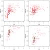 |
Fig. 22 Hardness ratios (left panels: HR1; right panels: HR2) vs. J−H, for all ACIS (bottom panels) and XMM-Newton (top panels) X-ray sources. Symbols as in Fig. 9. |
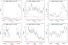 |
Fig. 23 Examples of (background-subtracted) X-ray light curves of XMM-Newton X-ray sources. The observations of sources in panels a) and d) have interruptions in the middle, hence their zero count rates there. The background count rate, scaled to the source area, is shown with red symbols. |
We also examined the X-ray lightcurves of sources detected with enough counts. Some examples are shown in Fig. 23, which illustrates the type of variability found. When the count rate is large enough, most sources are found to be variable; in many or most cases, lightcurve shapes are complex, while “simple” flares with impulsive rise and exponential decay are more rare. This is reminiscent of the X-ray lightcurves of YSOs in the ρ Oph star-forming region, from the XMM-Newton DROXO survey (Pillitteri et al. 2010). Panel e shows a probable (double-peaked) flare event, with a long decay time of ~10 ks, as found for example in the COUP Orion lightcurves (Favata et al. 2005). Some of the XMM-Newton observations have long interruptions in the middle (like in panels a and d). Large-amplitude variability on timescales of one day may also be seen from the comparison of the co-pointed ACIS-I images ObsId 13647 and 15592, already shown in Fig. 4.
Since X-ray emission decays with stellar age, one possible way of discriminating very young stars in the NAP from foreground and background active non-members is through the use of X-ray-to-optical luminosity ratios, which decrease with mass-dependent timescales (e.g., Preibisch & Feigelson 2005). Ratios of X-ray to bolometric (LX/Lbol) or X-ray to visual (LX/LV) luminosities are commonly used. In our case, the difficulty in obtaining accurate extinction values for individual X-ray sources makes these ratios unsuitable, and prompted us to search a reddening-free equivalent ratio. It is well known than while the dust absorption decreases from optical to IR wavelengths, the X-ray absorption decreases from the soft to the hard X-ray band, with photons of energy E = 2 keV being absorbed like NIR photons with λ = 2μ, for a typical interstellar gas-to-dust ratio. Therefore, we searched for an X-ray energy range where absorption is equivalent to that in the J NIR band, which as discussed above is convenient to study our NAP stars. We made several experiments using the PIMMS software2, for different energy bands: 0.8–1.2 keV, 1.0–1.8 keV, and 1.2–2.4 keV, sufficiently wide for being well characterized at the spectral resolution of Chandra/ACIS detector. Three single-temperature APEC thermal models were considered, in the temperature range of Class I/II/III YSOs. Hydrogen column density (NH) values were converted to optical extinction using the relation NH = 2.22 × 10²¹AV (Gorenstein 1975), while the correspondence between AV and NIR extinction is explained in Appendix C. The result of the experiment is shown in Fig. 24, where the ordinate shows the relative flux attenuation. We see that the X-ray band between 1.0–1.8 keV is absorbed by an amount similar to the J band, within a factor of ~50% up to AV ~ 10−12. Absorption in the harder 1.2–2.4 keV band is also very close to that in the H band; however, X-ray counts are often less in this higher-energy band than in the 1.0–1.8 keV band, and the NIR H band is more easily affected by non-photosperic contributions than the J band, so that the pair [1.0–1.8 keV]/J seems preferable to obtain an absorption-independent flux ratio.
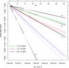 |
Fig. 24 Computed attenuation factors for X-ray and NIR emission and variable line-of-sight absorption, as parameterized by the hydrogen column density NH (bottom axis) and its equivalent extinction AV (top axis). X-ray attenuation of the observed ACIS-I flux is computed for three single-temperature emitting plasmas (short-dashed: 1 keV; mid-dashed: 1.5 keV; long-dashed: 2 keV), and three energy ranges, as labeled. Optical and NIR attenuation is shown (using the Aλ/AV conversions from Rieke & Lebosfky 1985) with the black solid lines. |
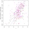 |
Fig. 25 ACIS-I count rate in the [1.0–1.8] keV band vs. J magnitude. The dashed and dotted lines represent proportionality; the distance between the dotted lines is an order magnitude difference in the X-ray to J flux ratio. Symbols as in Figs. 9 and 10, except for black crosses representing a spatially-selected subset of X-ray sources (see text). Arrows indicate count-rate upper limits to undetected RGS11 YSOs. |
A plot of X-ray count-rate in the 1.0–1.8 keV band vs. J is shown in Fig. 25, for ACIS-I sources with J−H < 2, corresponding roughly to AV = 12. In this diagram, absorption causes datapoints to move parallel to the dashed line, and might partially account for the correlation seen in the diagram, while the spread above and below that line reflects the X-ray to photospheric flux ratio. Most of the H58 stars have X-ray-to-NIR flux ratios within an order of magnitude. Their average ratio is also close to that of the bulk of NAP X-ray sources; only four of them show weaker X-ray-to-NIR flux ratio. Also the RGS11 YSOs appear well mixed with the non-YSO X-ray sources, and count-rate upper limits for X-ray undetected YSOs (arrows in the figure) are consistent with detections. The black crosses in the diagram are X-ray sources in the dashed rectangles in Figs. 20 and 21: also these sources do not appear to have particularly high or low X-ray-to-NIR flux ratios, and are therefore homogeneous with the rest of NAP X-ray sources.
We estimated X-ray luminosities LX for our X-ray sources, using PIMMS to compute conversion factors between count-rate and flux. These are weakly dependent on the emitting plasma temperature if this is above 1 keV, as often found in active PMS stars, but vary considerably as a function of NH, across the range of inferred absorption values for our NAP sources. As above, we estimated NH for individual sources from their J−H color, and using the above conversion between this and AV, and between AV and NH. Since we do not know individual distances for possible foreground stars, we might be overestimating LX for these latter. The derived LX distribution is shown in Fig. 26, for both the total NAP X-ray sample and selected subsamples. The total sample and the X-ray emitting M dwarfs are X-ray selected samples, and therefore do not include upper limits. For independently-selected samples such as H58 stars and RGS11 YSOs we instead computed individual LX upper limits using PW(X)Detect; these are used to compute maximum-likelihood X-ray luminosity functions, using the survival R software package3, shown in Fig. 26. With less than 20% of objects detected in X-rays, our sampling of the X-ray properties of flat-spectrum and Class I YSOs is rather poor, compared to the >60% X-ray detections among Class 0-I YSOs in the ONC by Prisinzano et al. (2008); nevertheless, the LX medians for the flat-spectrum and Class I YSOs from Fig. 26 fall very close to the LX median of Class 0-Ib objects in Prisinzano et al. (2008; we note that YSO classification was made differently by these authors and RGS11). The X-ray luminosity function of RGS11 Class II YSOs (33% detection rate) also has a median LX ~ 29.75 (erg/s), which compares well to the Preibisch & Feigelson (2005) results for the ONC M stars (median LX ~ 29.55 erg/s), but is significantly lower than the median LX of more massive stars in the ONC (or NGC 2264, or Chamaeleon: median LX ~ 29.9−30.5 erg/s). We have however found from our color-color diagrams that only a minor fraction of our X-ray sources are consistent with M-star colors. One possible solution to this contradiction is that we might be strongly underestimating absorption NH, and with it also LX, since we probably underestimated E(J−H) as discussed above, if these stars’ masses are much above ~0.5 M⊙. To test this, we computed the maximum E(J−H) (and corresponding NH) for each star, assuming an intrinsic value (J−H)0 = 0.15, appropriate to 1.4 M⊙ stars at 100 Myr (Fig. 15), but definitely not to 0.5 M⊙ stars: the resulting X-ray luminosity function for Class II YSOs is shown (dashed) in Fig. 26: the resulting median log LX ~ 30.1 is closer to the ONC value, and even more to the values for NGC 2264 and Chamaeleon stars in Preibisch & Feigelson (2005) for the mass range 0.5−0.9 M⊙, but remains a factor ~2 below the median LX for stars in the mass range 0.9−1.2 M⊙ in the same clusters, for which E(J−H)0 = 0.15 would be most appropriate. Therefore, reddening underestimates may be only a partial explanation of the low X-ray luminosity function of Class II objects in the NAP.
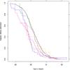 |
Fig. 26 Maximum-likelihood X-ray luminosity functions, for the entire NAP sample (black), and different subsamples: unreddened M dwarfs (blue), H58 stars (dark green), RGS11 YSOs of Class II (solid magenta), Class I (orange), and flat-spectrum YSOs (red). The dashed magenta distribution refers to Class II YSOs, using different absorption NH, see text. |
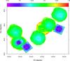 |
Fig. 27 Map of X-ray sensitivity across our survey. Color indicates log fx (top-axis scale, in units of erg s-1 cm-2), where fx is the minimum detectable X-ray flux at a reference energy of 1 keV. At the NAP distance, log fx = −15 corresponds to an (unabsorbed) X-ray luminosity log Lx ~ 28.6 erg/s. |
The H58 stars, most of which are not M stars, and which are only lightly absorbed, as seen above, have higher LX than the Class II YSOs (solid magenta line in Fig. 26), well consistent with PMS stars in the mass range M = 0.5−0.9 M⊙ from the different clusters shown by Preibisch & Feigelson (2005).
The unreddened M dwarfs have a LX distribution much lower than the bulk of NAP sources; if they are NAP members, the lower LX would not be surprising, since these stars are at the lower end of the mass spectrum (Fig. 19) and their LX distribution of Fig. 26 is close to that of similar-mass stars in the ONC (e.g., Preibisch & Feigelson 2005). However, we cannot rule out that these are M stars with ages similar to the Pleiades (~100 Myr), 3–10 times nearer to us, so that their actual LX would be 10–100 times lower than shown in Fig. 26: also in this case their LX distribution would agree with the data presented in Preibisch & Feigelson (2005; Fig. 4).
5.8. X-ray sensitivity limits
It is important to recognize to what extent the results presented above may be affected by the uneven sensitivity of the available X-ray data. As discussed in detail by Broos et al. (2011), two distinct causes contribute to the effect that an astrophysical object with a given intrinsic X-ray flux (at the NAP distance) may be detected or not. The first cause is instrumental, the detection sensitivity being not uniform across the imaged FOV, because of both mirror vignetting and PSF off-axis degradation. The second cause is of astrophysical origin and resides in the uneven column density of absorbing matter along the line of sight to the source, which was seen above to span a wide range inside the surveyed region. Therefore, we try here to quantitatively examine both effects individually.
The instrument-related effects are relatively easy to model, once the background level of each individual X-ray observation is measured, and properties like vignetting and PSF shape are known. If the spatial distribution of X-ray sources is wide enough, this gives rise to what is termed the “egg-crate effect” by Broos et al. (2011), since the smaller PSF near the (ACIS-I) FOV center results in a larger spatial density of detections there, with respect to FOV borders. We computed nominal minimum detectable fluxes fx (for point sources) for the entire NAP survey area using the capabilities of PW(X)Detect: the resulting map is shown in Fig. 27, including both ACIS and EPIC pointings. In order to compare different detectors in the same map, we cannot use purely instrumental quantities (counts/s), but physical ones, scaling counts to erg/cm2 with the adoption of the nominal instrument effective area at a representative energy of 1 keV. Since the two ACIS-I ObsIds 13647 and 15592 were analyzed together and the ACIS-S ObsId 14545 has higher sensitivity than ACIS-I datasets, all ACIS fields span approximately the same range of fx. Instead, the various XMM-Newton EPIC exposures are of unequal duration (see Table 1), and their fx is more sensitive to background than ACIS datasets: therefore, despite the more uniform PSF they collectively span a wider range of fx. This is more cleary seen in the fx histograms of Fig. 28, separately for ACIS and EPIC data: most of the width of the EPIC histogram is related to ObsId-to-ObsId variations, while most of the width of the ACIS histogram is related to center-to-border effects, the various ACIS FOV having similar fx ranges.
The strong center-to-border fx variation in ACIS datasets is responsible for the egg-crate effect, when this is found. However, the distribution of X-ray detections in NAP ACIS-I FOVs (Fig. 21) does not show such a centrally-symmetric shape, so we may conclude that any egg-crate effect is not primarily responsible for the observed spatial distribution of NAP X-ray sources. As far as other effects are concerned, it is interesting to observe from Fig. 25 (including only ACIS-I data) that upper limits span a wide range of almost two orders of magnitude, because they are computed on the basis of the individual source absorption values. The fact that they are even more frequent in the upper part of the diagram emphasizes that absorption, more than uneven detector properties, is the most important factor against their detection. This emerges also clearly from a comparison between the range in the ordinates of Fig. 25 of 2.5 orders of magnitude, and that spanned by the instrumental ACIS sensitivity (one order of magnitude) in the red histogram of Fig. 28.
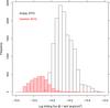 |
Fig. 28 Histograms of minimum detectable flux fx from the same spatial grid as in Fig. 27, shown separately for ACIS (red) and EPIC data (black). |
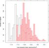 |
Fig. 29 Distribution of computed count-rate to flux conversion factors for all observed NIR objects (either X-ray detected of not), separately for ACIS (red) and EPIC (black) observations. |
The distribution of absorption-based (from J−H colors) X-ray count-rate-to-flux conversion factors is shown in Fig. 29, separately for ACIS and EPIC detectors (and regardless of whether each detector actually imaged a given source), under the same assumptions about the intrinsic source spectrum as in the previous subsection. For both instruments, the bulk of stars span approximately 1.5 orders of magnitude, in agreement with conclusions given just above. While the total NAP cloud absorption shows definite spatial properties (Fig. 17), the X-ray colors (Figs. 4 to 6) and NIR colors (Figs. 20 and 21) of X-ray sources are not generally correlated with the local total depth. This suggests that X-ray sources are located at various depths in the cloud, and the extrapolation of the undetected source density on the basis of the local density of detections is here at risk of being misleading. Such an approach, for example, is instead used by Kuhn et al. (2015) in their X-ray study of several massive SFRs, in which absorption is more uniform and source statistics (per FOV) is much higher than in the NAP, permitting a believable reconstruction of the undetected population. Contrarily to the data studied by Kuhn et al. (2015), in the NAP dataset the flux completeness limit (a flux above which we are confident to have detected near 100% of sources) is near the upper end of the detected source range, as can be understood from Fig. 25 where upper limits are found up to the top of the count-rate scale; this also renders the approach adopted by those authors unapplicable here. The conclusion drawn from Fig. 29 is that the intrinsic X-ray luminosities of undetected sources may range up to 1.5 orders of magnitude above their unabsorbed value, whose spatial distribution was shown in Fig. 27. The peaks of the instrumental-sensitivity and conversion-factor histograms, taken together, correspond to an intrinsic X-ray luminosity log Lx ~ 29.9 erg/s, detectable over most of the NAP fields. This Lx value being typical of low-mass PMS stars, we conclude that our NAP detection list can be considered representative of the young star population in this SFR.
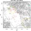 |
Fig. 30 Analogous of Fig. 21 (lower-left panel), but leaving out all X-ray detections with less than 15 counts. No optical or NIR objects are plotted here in order to show better the X-ray source distribution. The big yellow circles are Cambresy’s IR clusters, and the cyan star symbol is the O5 star, as in Fig. 21. |
While a proper reconstruction of the space and flux distributions of undetected NAP sources is unfeasible, we may nevertheless mitigate the instrumental effects described above, by considering only detections above a uniform threshold for a given X-ray FOV. Figure 30 shows the detected X-ray sources in the Gulf of Mexico ACIS FOV, already shown in Fig. 21 (lower-left panel), but limited to sources with more than 15 counts, and therefore detectable across the whole FOV (thus free from egg-crate effects). Although the source statistics becomes smaller, the non-uniform spatial distribution of detections is still clear, especially near one of the Cambresy’s NIR clusters. Therefore, the main conclusions of the previous subsections are not dramatically affected by instrumental factors.
6. Discussion
The results reported in the above sections emphasize once again the known complexity of the NAP star formation region, made of several subgroups of young stars (Cambrésy et al. 2002, RGS11), with no obvious connection between them. Although it was very difficult to assess individual membership for our X-ray detected sources, above results show that many (or most) of them exhibit properties (X-ray-to-NIR flux ratios, X-ray variability and spectrum hardness) consistent with young PMS stars. The non-detection in the X-rays of most YSOs, even those of Class II whose X-ray properties are best known, remains puzzling, since optical-NIR color-color diagrams seem to rule out for most of them the low mass values (M< 0.5 M⊙) that their X-ray luminosity function would imply. A better characterization of these objects would be desirable.
Perhaps the spatial distribution of our X-ray sources is our most interesting result. Although the illuminating O5 star 2MASS J20555125+4352246 does not fall in any of our X-ray FOVs, we observed its immediate neighborhood, a few arcmin away from it: there is no sign of any concentration of X-ray sources around it, in agreement with the finding by its discoverers that it is remarkably isolated (Comerón & Pasquali 2005). This isolation refers therefore not only to comparably massive stars, but to stars down to solar-like masses, to which our survey is sensitive even at the extinction of the O5 star. This is very different from most star-forming regions, where the highest-mass stars are immediately surrounded by low-mass PMS stars. It would be interesting to investigate if this is a runaway star, with implications on the timescales on which it might have interacted with the molecular cloud; although no such information is available now, the Gaia data should provide it in a short time frame.
The two sub-regions with the highest YSO spatial density, the Gulf of Mexico and Pelican, are also those with the largest number of X-ray detections (although this might be somewhat biased by having used there the most sensitive ACIS detectors). In the Gulf of Mexico, closest to the O5 star, there is a clear spatial trend: YSOs are clustered near the border of the dark cloud which faces the O star (and not inside the cloud), and tens of X-ray sources follow the same pattern; moreover, several other tens X-ray sources are found between the YSO cluster(s) and the O star, forming an apparently distinct layer. It is interesting to remark that in Fig. 20 of RGS11 the Class III stars fall in this same intermediate region. This is highly suggestive of a time sequence, with formation of stars proceeding southwards, under the strong influence of the massive O star nearby. The X-ray sources without a YSO counterpart, as well as the Class III stars, would thus be the oldest, with younger stars being currently formed in the outer layers of the dense dust cloud. Toujima et al. (2011) also suggest triggered star formation in NGC 7000, on the basis of molecular-line observations. The disk-free X-ray detected stars are not necessarily much older than the others (no such separation is found in our de-reddened CMD), since when exposed to strong UV irradiation disk lifetimes are likely to be significantly shortened (e.g., Guarcello et al. 2007, 2009). In other places in the NAP, a similar segregation between the YSO and X-ray source distributions is observed, as in the Pelican hat, but its origin is much less clear, since the triggerer of the possible time sequence is not obvious. Moreover, we recover at least three of the Cambrésy et al. (2002) NIR clusters in X-rays, confirming their existence.
The assessment of membership for the X-ray detected sources was difficult, as discussed above for each of the possible indicators. Only ~29% of all X-ray sources have Hα or NIR excesses (either from this work or from RGS11 and H58), and are therefore high-probability members individually. Most other X-ray sources have however X-ray properties, colors and extinction very similar to the former, and are probable members as well. The foreground extinction toward the NAP is very small, as we find from color-color diagrams and in agreement with Laugalys et al. (2006, 2007), and therefore foreground X-ray sources may only be found at near-zero reddening: we found only a few tens such sources above. Extinction rises rather abruptly in the NAP, although this may be position-dependent as we have examined above (in agreement with Cambrésy et al. 2002). Background X-ray sources, behind such large absorbing column, are unlikely to be coronal sources, but may be distant compact objects or even AGNs, both characterized by large X-ray-to-optical flux ratios. We tentatively identify these classes of sources with our unidentified X-ray sources (115 out of 721 total detections), which must have large X-ray-to-optical flux ratios if they are missed in both of the very deep IPHAS and UKIDSS catalogs. To summarize, most of the NAP X-ray sources with an optical or NIR counterpart, except perhaps a significant fraction of the unreddened ones, are good candidates as young NAP members.
7. Summary
We have performed the first extensive, wide-area X-ray survey of the North-America and Pelican star-forming region, using both Chandra/ACIS and XMM-Newton/EPIC detectors. More than 700 unique X-ray sources have been detected, of which ~85% have a counterpart in at least one of the IPHAS, UKIDSS or 2MASS catalogs. Only ~29% of X-ray sources are identified with previously known YSOs or CTTS, or with newly found Hα-emission or NIR-excess stars. We argued that most of the X-ray sources identified with an optical or NIR counterpart are probable members of the star-forming region. A few tens unreddened X-ray sources are probable active foreground low-mass stars.
In the Gulf-of-Mexico region, the respective spatial properties of dark obscuration, YSOs, and X-ray sources without YSO association are suggestive of a sequential star-formation scenario, with the O5 star illuminating the entire nebula as the probable triggerer. Unlike most star-forming regions, this most massive star appears isolated even in X-ray images. The large-scale spatial distribution of the X-ray detected member candidates follows qualitatively that of the known YSOs, with several sub-clusters, apparently physically unconnected.
Detailed follow-up (spectroscopic) observations will be needed to confirm individual membership of the X-ray sources found here.
The XMM-Newton EPIC camera sensitivity dependence on off-axis distance is flat enough that such a central concentration of detections cannot be an instrumental effect.See also Sect. 5.8.
Portable, Interactive Multi-Mission Simulator, available at http://heasarc.gsfc.nasa.gov/docs/software/tools/pimms.html
Acknowledgments
We wish to thank an anonymous referee for his/her helpful suggestions. I.P. acknowledges support by Chandra fund 16617814 contract GO2-13021X. The scientific results reported in this article are based on observations made by the Chandra and XMM-Newton X-ray Observatories. This paper also makes use of data obtained as part of the INT Photometric Hα Survey of the Northern Galactic Plane (IPHAS, www.iphas.org) carried out at the Isaac Newton Telescope (INT). The INT is operated on the island of La Palma by the Isaac Newton Group in the Spanish Observatorio del Roque de los Muchachos of the Instituto de Astrofisica de Canarias. All IPHAS data are processed by the Cambridge Astronomical Survey Unit, at the Institute of Astronomy in Cambridge. The bandmerged DR2 catalog was assembled at the Centre for Astrophysics Research, University of Hertfordshire, supported by STFC grant ST/J001333/1. This publication makes use of data products from the Wide-field Infrared Survey Explorer, which is a joint project of the University of California, Los Angeles, and the Jet Propulsion Laboratory/California Institute of Technology, funded by the National Aeronautics and Space Administration. This research makes use of the SIMBAD database, operated at CDS, Strasbourg, France. We also make heavy use of R: A language and environment for statistical computing. R Foundation for Statistical Computing, Vienna, Austria. (http://www.R-project.org/).
References
- Armond, T., Reipurth, B., Bally, J., & Aspin, C. 2011, A&A, 528, A125 [NASA ADS] [CrossRef] [EDP Sciences] [Google Scholar]
- Aspin, C. 2011, AJ, 141, 196 [NASA ADS] [CrossRef] [Google Scholar]
- Bally, J., & Reipurth, B. 2003, AJ, 126, 893 [NASA ADS] [CrossRef] [Google Scholar]
- Bally, J., Ginsburg, A., Probst, R., et al. 2014, AJ, 148, 120 [NASA ADS] [CrossRef] [Google Scholar]
- Baraffe, I., Homeier, D., Allard, F., & Chabrier, G. 2015, A&A, 577, A42 [NASA ADS] [CrossRef] [EDP Sciences] [Google Scholar]
- Barentsen, G., Farnhill, H. J., Drew, J. E., et al. 2014, MNRAS, 444, 3230 [NASA ADS] [CrossRef] [Google Scholar]
- Broos, P. S., Townsley, L. K., Feigelson, E. D., et al. 2011, ApJS, 194, 2 [NASA ADS] [CrossRef] [Google Scholar]
- Cambrésy, L., Beichman, C. A., Jarrett, T. H., & Cutri, R. M. 2002, AJ, 123, 2559 [NASA ADS] [CrossRef] [Google Scholar]
- Comerón, F., & Pasquali, A. 2005, A&A, 430, 541 [NASA ADS] [CrossRef] [EDP Sciences] [Google Scholar]
- Corbally, C. J., Straižys, V., & Laugalys, V. 2009, Balt. Astron., 18, 111 [NASA ADS] [Google Scholar]
- Covey, K. R., Hillenbrand, L. A., Miller, A. A., et al. 2011, AJ, 141, 40 [NASA ADS] [CrossRef] [Google Scholar]
- Damiani, F., Maggio, A., Micela, G., & Sciortino, S. 1997a, ApJ, 483, 350 [NASA ADS] [CrossRef] [Google Scholar]
- Damiani, F., Maggio, A., Micela, G., & Sciortino, S. 1997b, ApJ, 483, 370 [NASA ADS] [CrossRef] [Google Scholar]
- Damiani, F., Prisinzano, L., Micela, G., & Sciortino, S. 2006, A&A, 459, 477 [NASA ADS] [CrossRef] [EDP Sciences] [Google Scholar]
- Dunham, M. M., Arce, H. G., Bourke, T. L., et al. 2012, ApJ, 755, 157 [NASA ADS] [CrossRef] [Google Scholar]
- Drew, J. E., Greimel, R., Irwin, M. J., et al. 2005, MNRAS, 362, 753 [NASA ADS] [CrossRef] [Google Scholar]
- Drew, J. E., Gonzalez-Solares, E., Greimel, R., et al. 2014, MNRAS, 440, 2036 [NASA ADS] [CrossRef] [Google Scholar]
- Favata, F., & Micela, G. 2003, Space Sci. Rev., 108, 577 [Google Scholar]
- Favata, F., Flaccomio, E., Reale, F., et al. 2005, ApJS, 160, 469 [NASA ADS] [CrossRef] [Google Scholar]
- Gorenstein, P. 1975, ApJ, 198, 95 [NASA ADS] [CrossRef] [Google Scholar]
- Green, J. D., Evans, N. J., II, Kóspál, Á., et al. 2011, ApJ, 731, L25 [NASA ADS] [CrossRef] [Google Scholar]
- Guarcello, M. G., Prisinzano, L., Micela, G., et al. 2007, A&A, 462, 245 [NASA ADS] [CrossRef] [EDP Sciences] [Google Scholar]
- Guarcello, M. G., Micela, G., Damiani, F., et al. 2009, A&A, 496, 453 [NASA ADS] [CrossRef] [EDP Sciences] [Google Scholar]
- Guarcello, M. G., Damiani, F., Micela, G., et al. 2010, A&A, 521, A18 [NASA ADS] [CrossRef] [EDP Sciences] [Google Scholar]
- Güdel, M., Guinan, E. F., & Skinner, S. L. 1997, ApJ, 483, 947 [NASA ADS] [CrossRef] [Google Scholar]
- Guieu, S., Rebull, L. M., Stauffer, J. R., et al. 2009, ApJ, 697, 787 [NASA ADS] [CrossRef] [Google Scholar]
- Herbig, G. H. 1958, ApJ, 128, 259 [NASA ADS] [CrossRef] [Google Scholar]
- Hodgkin, S. T., Irwin, M. J., Hewett, P. C., & Warren, S. J. 2009, MNRAS, 394, 675 [NASA ADS] [CrossRef] [Google Scholar]
- Kalari, V. M., Vink, J. S., Drew, J. E., et al. 2015, MNRAS, 453, 1026 [NASA ADS] [CrossRef] [Google Scholar]
- Kóspál, Á., Ábrahám, P., Acosta-Pulido, J. A., et al. 2011, A&A, 527, A133 [NASA ADS] [CrossRef] [EDP Sciences] [Google Scholar]
- Kuhn, M. A., Getman, K. V., & Feigelson, E. D. 2015, ApJ, 802, 60 [NASA ADS] [CrossRef] [Google Scholar]
- Laugalys, V., Straižys, V., Vrba, F. J., et al. 2006a, Balt. Astron., 15, 327 [NASA ADS] [Google Scholar]
- Laugalys, V., Straižys, V., Vrba, F. J., et al. 2006b, Balt. Astron., 15, 483 [NASA ADS] [Google Scholar]
- Laugalys, V., Straižys, V., Vrba, F. J., et al. 2007, Balt. Astron., 16, 349 [NASA ADS] [Google Scholar]
- Lawrence, A., Warren, S. J., Almaini, O., et al. 2007, MNRAS, 379, 1599 [NASA ADS] [CrossRef] [MathSciNet] [Google Scholar]
- Lee, J.-E., Park, S., Green, J. D., et al. 2015, ApJ, 807, 84 [NASA ADS] [CrossRef] [Google Scholar]
- Liebhart, A., Güdel, M., Skinner, S. L., & Green, J. 2014, A&A, 570, L11 [NASA ADS] [CrossRef] [EDP Sciences] [Google Scholar]
- Lin, D., Webb, N. A., & Barret, D. 2012, ApJ, 756, 27 [NASA ADS] [CrossRef] [Google Scholar]
- Miller, A. A., Hillenbrand, L. A., Covey, K. R., et al. 2011, ApJ, 730, 80 [NASA ADS] [CrossRef] [Google Scholar]
- Pillitteri, I., Sciortino, S., Flaccomio, E., et al. 2010, A&A, 519, A34 [NASA ADS] [CrossRef] [EDP Sciences] [Google Scholar]
- Pillitteri, I., Wolk, S. J., Megeath, S. T., et al. 2013, ApJ, 768, 99 [NASA ADS] [CrossRef] [Google Scholar]
- Preibisch, T., & Feigelson, E. D. 2005, ApJS, 160, 390 [NASA ADS] [CrossRef] [Google Scholar]
- Prisinzano, L., Damiani, F., Micela, G., & Sciortino, S. 2005, A&A, 430, 941 [NASA ADS] [CrossRef] [EDP Sciences] [Google Scholar]
- Prisinzano, L., Micela, G., Flaccomio, E., et al. 2008, ApJ, 677, 401 [NASA ADS] [CrossRef] [Google Scholar]
- Rebull, L. M., Guieu, S., Stauffer, J. R., et al. 2011, ApJS, 193, 25 [NASA ADS] [CrossRef] [Google Scholar]
- Reipurth, B., & Schneider, N. 2008, in Handbook of Star Forming Regions, ASP Monograph Publ., Vol. 4, 36 [Google Scholar]
- Rieke, G. H., & Lebofsky, M. J. 1985, ApJ, 288, 618 [NASA ADS] [CrossRef] [Google Scholar]
- Semkov, E. H., Peneva, S. P., Munari, U., Milani, A., & Valisa, P. 2010, A&A, 523, L3 [NASA ADS] [CrossRef] [EDP Sciences] [Google Scholar]
- Semkov, E. H., Peneva, S. P., Munari, U., et al. 2012, A&A, 542, A43 [NASA ADS] [CrossRef] [EDP Sciences] [Google Scholar]
- Skinner, S. L., Briggs, K. R., Guedel, M., & Sokal, K. R. 2007, BAAS, 39, 62.27 [Google Scholar]
- Straižys, V., Corbally, C. J., & Laugalys, V. 2008, Balt. Astron., 17, 125 [Google Scholar]
- Toujima, H., Nagayama, T., Omodaka, T., et al. 2011, PASJ, 63, 1259 [NASA ADS] [CrossRef] [Google Scholar]
- Welin, G. 1973, A&AS, 9, 183 [NASA ADS] [Google Scholar]
- Witham, A. R., Knigge, C., Drew, J. E., et al. 2008, MNRAS, 384, 1277 [NASA ADS] [CrossRef] [Google Scholar]
- Wright, E. L., Eisenhardt, P. R. M., Mainzer, A. K., et al. 2010, AJ, 140, 1868 [NASA ADS] [CrossRef] [Google Scholar]
Appendix A: 2MASS – UKIDSS calibration
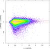 |
Fig. A.1 2MASS-UKIDSS comparison: difference J2MASS−JUKIDSS vs. UKIDSS J−H color (2D histogram). The black dashed line represents J2MASS−JUKIDSS = 0, while the red solid line is a best-fit to the data. |
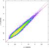 |
Fig. A.2 Comparison between J−H colors from 2MASS and UKIDSS. The black dashed line represents (J−H)2MASS = (J−H)UKIDSS, while the red solid line is a best-fit to the data. |
The UKIDSS J,H,K photometric system is calibrated to the 2MASS system (Hodgkin et al. 2009); however, the calibration was made at low reddening, and we find that small adjustments are required to match the two catalogs at large reddening values, typical of the NGC 7000/IC 5070 region. The difference between 2MASS and UKIDSS J magnitudes is shown in Fig. A.1: although small, this difference is often significant compared to the very small errors in the UKIDSS magnitudes. Only objects with errors <0.07 mag in both J bands, and errors < 0.1 mag in (J−H)UKIDSS, are shown. A least-square fit to the data (with fixed zero intercept) has the form:  (A.1)The J−H colors differ between 2MASS and UKIDSS more appreciably, however, by almost 8% (Fig. A.2, where only objects with errors <0.1 mag in both (J−H)UKIDSS and (J−H)2MASS are shown). The best fit to the data (with zero intercept) has the form:
  (A.2)Similarly, Fig. A.3 shows the comparison between the respective H−K colors, with the best fit here given by:
  (A.3)All UKIDSS magnitudes were therefore rescaled according to the (J−H)UKIDSS color, to match the 2MASS photometric system even at large reddening. At low reddening (low J−H), this recalibration is irrelevant, and does not interfere with the one presented by Hodgkin et al. (2009). After recalibration, we merged the 2MASS and UKIDSS catalogs into a single NIR source catalog, choosing the more precise UKIDSS magnitudes when available.
Appendix B: IPHAS – VPHAS+ calibration
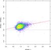 |
Fig. B.1 IPHAS-VPHAS+ comparison: difference rIPHAS−rVPHAS vs. VPHAS+r−i color (2D histogram). The black dashed line represents rIPHAS−rVPHAS = 0, while the red solid line is a best-fit to the data. |
Although the IPHAS r,i photometric system is similar to the Sloan Survey system, the formulae in Barentsen et al. (2014) indicate that significant differences exist between the two systems. Moreover, no recipe is given to convert the IPHAS r,i magnitudes into Johnson/Cousins VRI magnitudes. Such a recipe is instead given by Drew et al. (2014) for the VPHAS+ugri magnitudes, which are closely related to the IPHAS filter system. The BHAC evolutionary tracks and isochrones, moreover, are currently available for the VRI filters, but not for either the Sloan or the IPHAS (or VPHAS+) filters, so we attempt here to recalibrate the IPHAS r,i magnitudes in terms of the VPHAS+r,i, whose relation with VRI is known from Drew et al. (2014). We consider an equatorial field where both IPHAS and VPHAS+ data are available, to study their photometric differences. The results of this experiment are shown in Figs. B.1 and B.2, where only objects with errors <0.05 mag in all bands are shown. The best-fit relations shown in these figures are:
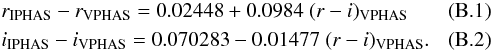
These relations (together with those given in Drew et al. 2014) were used to convert the BHAC tracks and isochrones in the Johnson/Cousins filters into the appropriate IPHAS r,i magnitudes and colors.
Appendix C: Reddening law
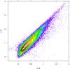 |
Fig. C.1 Slope of reddening vector (E(J−H) /E(H−K) = 1.9) in the (J−H,H−K) plane (red line), obtained from the giant-star sequence, which is best seen from the iso-density contours (black). |
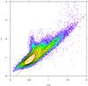 |
Fig. C.2 Same as Fig. C.1, for the (r−i,J−H) plane: here the reddened giant-star sequence is particularly well distinct from the reddened main sequence, while the unreddened M-dwarf locus protrudes upwards near J−H ~ 0.6. The reddening-vector slope is here E(r−i) /E(J−H) = 1.79. |
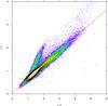 |
Fig. C.3 Same as Fig. C.1, for the (r−i,i−J) plane: the reddening-vector slope is here E(r−i) /E(i−J) = 0.6. |
We study here the empirical reddening law for the NGC 7000/IC 5070 region, in the r,i,J,H,K bands. With respect to previous studies, we benefit here from an extensive optical and NIR catalog, reaching down to faint magnitudes with small photometric errors. Thanks to these properties, we are able to discern in several color-color diagrams the giant-star locus from the dwarfs locus. Figure C.1 shows the (J−H,H−K) diagram of all sources in the studied region: the reddened red-giant sequence starts at J−H ~ 0.8, whereas the dwarf sequence starts at J−H ~ 0, but the giants being more luminous remain observable up to larger reddening values. We
have therefore visually fitted the giant sequence with the red line in the figure (with slope E(J−H) /E(H−K) = 1.9). It should be remarked that at low reddening dwarfs dominate the distribution because of their higher spatial density, but at large reddening giants dominate being observable up to larger distances: it is therefore incorrect to derive the reddening vector slope by simply joining the low and high ends of the color distribution with a straight line, since this would mix together stars with different intrinsic NIR colors, and the resulting slope would be higher than the true one. The upper envelope of datapoints in the figure also agrees with the slope we estimate from the giant sequence.
Figure C.2 is a mixed optical-NIR (r−i,J−H) diagram, where we can discern well the reddened giant sequence (the lowest one, including the highest-reddening stars) from the dwarf sequence. Protruding upwards, the M-dwarf sequence is also clearly seen (cf. Fig. 12). The reddening vector has a slope of E(r−i) /E(J−H) = 1.79.
In the (r−i,i−J) diagram of Fig. C.3, instead, the dwarf and giant sequence are not distinct, but the M-dwarfs are. The reddening-vector slope is here E(r−i) /E(i−J) = 0.6.
In order to connect these reddening laws to the V-band extinction, and to obtain the total-to-selective extinction ratio Ai/E(r−i) for the IPHAS filters, we need two more equations. Assuming that the J band is least affected by peculiar reddening laws, we therefore take from Rieke & Lebofsky (1985) the ratios AJ/AV = 0.282 and E(J−H) /AV = 0.107. The set of relative extinctions Aλ/AV for the NAP thus becomes:
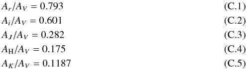
where Eqs. (C.3) and (C.4) are merely the Rieke & Lebofsky (1985) relations, included for convenience.
All Tables
All Figures
|
Fig. 1 Digital-Sky-Survey II red image of the North-America and Pelican nebulae (inverted grayscale), with overlaid the regions covered by XMM-Newton observations (big circles), and Chandra ACIS observations (squares), each labeled with its ObsId number. X-ray fields of view are drawn in red for new data, and black for archive data. ACIS-I ObsIds 13467 and 15592 share the same pointing direction and roll angle. Archive XMM ObsIds 0656780701 and 0656781201 also share the same pointing direction, but with a slightly different roll angle; only 0656780701 is labeled in the figure. Small green squares are the H58 emission-line stars; blue crosses are YSOs from RGS11. Yellow circles indicate positions and approximate sizes of the Cambrésy et al. (2002) clusters of 2MASS NIR sources. The three bigger star symbols indicate respectively the O5 star 2MASS J20555125+4352246 (cyan), the FU Ori object candidate HBC722 (=V2493 Cyg = 2MASS J20581702+4353433, green), and the FU Ori star V1057 Cyg (=2MASS J20585371+4415283, orange). |
| In the text | |
|
Fig. 2 True-color WISE image of the region. Red: 22μ, green: 12μ, and blue: 4.6μ channels, respectively. The big circles and squares indicate the X-ray FOVs as in Fig. 1. North is up and east to the left. At a distance of 560 pc, the 3-degree sky region shown measures 29.3 pc on a side. |
| In the text | |
|
Fig. 3 Optical emission-line image of part of the region (courtesy Ondřej Podlucký, http://astrofotky.cz), in the lines of [O III] (blue), Hα (green) and [S II] (red), showing increasing ionization toward a location behind the obscuring dust. The white arrow indicates north. |
| In the text | |
|
Fig. 4 True-color X-ray images of individual observations, slightly smoothed to emphasize point sources. Red: 0.4–1.2 keV; green: 1.2–2.4 keV; blue: 2.4–7.9 keV. Panel a), upper left: ACIS-I ObsId 13648 (in the Gulf of Mexico). The ACIS-I FOV size is 16.9 arcmin on a side. b), upper right: ACIS-I ObsId 13647 (“Pelican”). c), lower left: ACIS-I ObsId 15592, with same pointing as ObsId 13647 (panel b)). Comparison with this latter ObsId makes source variability very evident. d), lower right: XMM-Newton ObsId 0679580101 (“Pelican hat”). In all XMM-Newton images shown here, MOS1, 2 and PN data are combined together. |
| In the text | |
|
Fig. 5 X-ray images as in Fig. 4. Panel a), upper left: XMM-Newton ObsId 0679580201. The brightest source (2XMM J205347.0+442301) (classified as a star by Lin et al. 2012) produces both diffraction spikes and a stripe of out-of-time events, accumulated during CCD readout. The white line outlines the eastern part of ACIS ObsId 13647 FOV. b), upper right: XMM-Newton ObsId 0679580301, toward the highly obscured region LDN 935. The plus sign labeled “O5” is the O star 2MASS J20555125+4352246 from Comerón & Pasquali (2005). c), lower left: archive ACIS-S ObsId 14545. The two white squares indicate ACIS-S chips 6 (front-illuminated, right) and 7 (back-illuminated, left), which have different sensitivities and are analyzed separately. This ObsId also has data from chips 2, 3, and 8, shown in the same figure; however the sensitivity and spatial resolution of these chips is inferior, and they are not considered further here. Near the center of the image, the green plus sign indicates the new FU Ori candidate HBC 722. To the SW a part of ACIS 13648 FOV can be seen. d), lower right: Archive XMM-Newton ObsId 0302640201, just north of ACIS-S ObsId 14545 (seen in lower-right corner). Near image center the FU Ori star V1057 Cyg is labeled. |
| In the text | |
|
Fig. 6 X-ray images as in Fig. 4. Panel a), left: Archive XMM-Newton ObsId 0556050101, overlapping XMM ObsId 0679580201 of Fig. 5, panel a). The bright source is the same as in that figure. The distribution of background emission seen here is caused by the small-window mode used here for the MOS cameras (not for the PN camera). b), right: archive XMM-Newton ObsId 0656780701+0656781201. The slight pointing difference between the two ObsIds causes the inter-chip gap pattern seen in the figure. The image overlaps completely with the ACIS 14545 FOV, and partially with ACIS 13648 FOV in the lower right corner. The tight group of X-ray sources surrounding HBC 722 (Fig. 5, panel c)) is unresolved here. |
| In the text | |
|
Fig. 7 Same field and background image as in Fig. 1, with small symbols now indicating: X-ray detected sources (red crosses), near-IR excess objects (orange triangles), and Hα-excess objects (dark-red circles). Big circles and squares are X-ray FOVs as in Fig. 1. |
| In the text | |
|
Fig. 8 An (i,r−i) CMD of stars toward two heavy-obscuration regions in LDN 935, with a 10-Gyr isochrone from BHAC at zero reddening and distance of 560 pc (bluesolid curve).Blue dashed curves correspond to distances smaller and larger by 20%, respectively. Only datapoints with errors <0.05 on both i and r−i are shown. |
| In the text | |
|
Fig. 9 IPHAS (r−Hα,r−i) diagram. The grayscale background is a 2D histogram of all IPHAS objects in the sky region of Fig. 1, with bin sizes of 0.01 in both axes. The dashed line is the CTTS-star limit. Symbols as in Fig. 7, with the addition of YSOs from RGS11 (violet squares), and emission-line stars from H58 (dark-green squares). Hundreds of faint stars above the dashed line are not selected here as Hα-emission stars because of their position in the CMD. |
| In the text | |
|
Fig. 10 Near-IR color-color diagram (J−H,H−K), using both 2MASS and UKIDSS data. Symbols as in Fig. 9. The arrow indicates the reddening vector corresponding to AV = 1. The dashed line is the adopted limit to select NIR-excess objects from this diagram. The blue lines in the lower-left part are unreddened BHAC isochrones for ages of 1, 3, 10, 30, 100 Myr, and 10 Gyr, and masses between 0.08−1.4 M⊙. BHAC evolutionary tracks for masses of 0.1, 0.3, and 0.5 M⊙ are shown in green.In this and following color-color diagrams, only data with errors less than 0.1 mag on each color are shown. |
| In the text | |
|
Fig. 11 Optical-IR color-color diagram (r−i,H−K). Symbols as in Figs. 9 and 10. The dashed line is the adopted limit for selection of NIR-excess objects from this particular diagram. The magenta thick line in the lower-left part indicates the location of unreddened stars in the mass range 1−1.4 M⊙. Much larger fractions of the H58 stars and of the RGS11 YSOs show a NIR excess using this diagram, compared to that of Fig. 10. |
| In the text | |
|
Fig. 12 Optical-IR color-color diagram (r−i,J−H). Symbols as in Figs. 9 and 10. The dashed line is the adopted limit for selection of NIR-excess objects from this particular diagram. |
| In the text | |
|
Fig. 13 Optical-IR color-color diagram (r−i,i−H). Symbols as in Figs. 9 and 10. Stars less massive than 0.5 M⊙ (M-type) fall above the dashed line. |
| In the text | |
|
Fig. 14 Optical color-magnitude diagram (i,r−i). Symbols as in Figs. 9 and 10. Unreddened BHAC evolutionary tracks are here shown for masses of 0.1, 0.2, 0.3, 0.5, 0.7 M⊙ (green), and 1 M⊙ (magenta).In this and following color-magnitude diagrams, only data with errors less than 0.1 mag on each axis are shown. |
| In the text | |
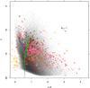 |
Fig. 15 NIR color-magnitude diagram (J,J−H). Symbols as in Figs. 9 and 10. |
| In the text | |
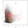 |
Fig. 16 NIR color-magnitude diagram (H,H−K). Symbols as in Figs. 9 and 10. |
| In the text | |
|
Fig. 17 Spatial map of average J−H (scale at figure top) as a measure of extinction. Indicated are the X-ray FOVs as in Fig. 1. The datapoints indicate X-ray sources (red) and RGS11 YSOs (orange). |
| In the text | |
|
Fig. 18 Mixed color-color diagram of r−i vs. corrected color (J−H)c (see text). Symbols as in Figs. 9 and 10. The vertical dotted line indicates the value (J−H)c = 0.75. |
| In the text | |
|
Fig. 19 De-reddened optical CMD. Symbols, isochrones and evolutionary tracks as in Fig. 14. The black plus signs are the unreddened M stars from Fig. 13 (with 2 < (i−H) < 3). |
| In the text | |
|
Fig. 20 Comparison between spatial distributions of X-ray sources, YSOs and other young stars in each X-ray FOV. The background grayscale image is a 2D histogram of the combined optical-NIR object density, showing clearly high-obscuration regions. Solid black circles and squares are XMM and ACIS FOVs, respectively. Symbols as in Figs. 9 and 10, except that here X-ray sources (crosses) are color-coded according to their J−H color (with the color scale show in the top left panel). X-ray sources without a NIR counterpart are shown in red. Black plus signs indicate positions of all RGS11 YSOs, regardless of their identification with X-ray or other cataloged objects. Small empty circles are young stars from Armond et al. (2011; black) and Welin (1973; violet). Yellow circles are 2MASS star clusters from Cambrésy et al. (2002). The black dashed rectangular regions are defined here as places with a local overdensity of X-ray sources, not matched by an overdensity of YSOs. The three bigger star symbols indicate respectively the O5 star 2MASS J20555125+4352246 (cyan), and FUOrs HBC722 (green) and V1057 Cyg (orange). |
| In the text | |
|
Fig. 21 Continuation of Fig. 20. In the lower-right panel the zooming factor is much larger than in the other panels, to help visually resolve the dense cluster in the center. The 2D bin size of the background image (and the density-grayscale conversion) is the same in all panels here and in Fig. 20. |
| In the text | |
|
Fig. 22 Hardness ratios (left panels: HR1; right panels: HR2) vs. J−H, for all ACIS (bottom panels) and XMM-Newton (top panels) X-ray sources. Symbols as in Fig. 9. |
| In the text | |
|
Fig. 23 Examples of (background-subtracted) X-ray light curves of XMM-Newton X-ray sources. The observations of sources in panels a) and d) have interruptions in the middle, hence their zero count rates there. The background count rate, scaled to the source area, is shown with red symbols. |
| In the text | |
|
Fig. 24 Computed attenuation factors for X-ray and NIR emission and variable line-of-sight absorption, as parameterized by the hydrogen column density NH (bottom axis) and its equivalent extinction AV (top axis). X-ray attenuation of the observed ACIS-I flux is computed for three single-temperature emitting plasmas (short-dashed: 1 keV; mid-dashed: 1.5 keV; long-dashed: 2 keV), and three energy ranges, as labeled. Optical and NIR attenuation is shown (using the Aλ/AV conversions from Rieke & Lebosfky 1985) with the black solid lines. |
| In the text | |
|
Fig. 25 ACIS-I count rate in the [1.0–1.8] keV band vs. J magnitude. The dashed and dotted lines represent proportionality; the distance between the dotted lines is an order magnitude difference in the X-ray to J flux ratio. Symbols as in Figs. 9 and 10, except for black crosses representing a spatially-selected subset of X-ray sources (see text). Arrows indicate count-rate upper limits to undetected RGS11 YSOs. |
| In the text | |
|
Fig. 26 Maximum-likelihood X-ray luminosity functions, for the entire NAP sample (black), and different subsamples: unreddened M dwarfs (blue), H58 stars (dark green), RGS11 YSOs of Class II (solid magenta), Class I (orange), and flat-spectrum YSOs (red). The dashed magenta distribution refers to Class II YSOs, using different absorption NH, see text. |
| In the text | |
|
Fig. 27 Map of X-ray sensitivity across our survey. Color indicates log fx (top-axis scale, in units of erg s-1 cm-2), where fx is the minimum detectable X-ray flux at a reference energy of 1 keV. At the NAP distance, log fx = −15 corresponds to an (unabsorbed) X-ray luminosity log Lx ~ 28.6 erg/s. |
| In the text | |
|
Fig. 28 Histograms of minimum detectable flux fx from the same spatial grid as in Fig. 27, shown separately for ACIS (red) and EPIC data (black). |
| In the text | |
|
Fig. 29 Distribution of computed count-rate to flux conversion factors for all observed NIR objects (either X-ray detected of not), separately for ACIS (red) and EPIC (black) observations. |
| In the text | |
|
Fig. 30 Analogous of Fig. 21 (lower-left panel), but leaving out all X-ray detections with less than 15 counts. No optical or NIR objects are plotted here in order to show better the X-ray source distribution. The big yellow circles are Cambresy’s IR clusters, and the cyan star symbol is the O5 star, as in Fig. 21. |
| In the text | |
|
Fig. A.1 2MASS-UKIDSS comparison: difference J2MASS−JUKIDSS vs. UKIDSS J−H color (2D histogram). The black dashed line represents J2MASS−JUKIDSS = 0, while the red solid line is a best-fit to the data. |
| In the text | |
|
Fig. A.2 Comparison between J−H colors from 2MASS and UKIDSS. The black dashed line represents (J−H)2MASS = (J−H)UKIDSS, while the red solid line is a best-fit to the data. |
| In the text | |
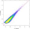 |
Fig. A.3 Same as Fig. A.2, for H−K. |
| In the text | |
|
Fig. B.1 IPHAS-VPHAS+ comparison: difference rIPHAS−rVPHAS vs. VPHAS+r−i color (2D histogram). The black dashed line represents rIPHAS−rVPHAS = 0, while the red solid line is a best-fit to the data. |
| In the text | |
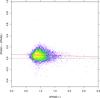 |
Fig. B.2 Same as Fig. B.1, for the i band. |
| In the text | |
|
Fig. C.1 Slope of reddening vector (E(J−H) /E(H−K) = 1.9) in the (J−H,H−K) plane (red line), obtained from the giant-star sequence, which is best seen from the iso-density contours (black). |
| In the text | |
|
Fig. C.2 Same as Fig. C.1, for the (r−i,J−H) plane: here the reddened giant-star sequence is particularly well distinct from the reddened main sequence, while the unreddened M-dwarf locus protrudes upwards near J−H ~ 0.6. The reddening-vector slope is here E(r−i) /E(J−H) = 1.79. |
| In the text | |
|
Fig. C.3 Same as Fig. C.1, for the (r−i,i−J) plane: the reddening-vector slope is here E(r−i) /E(i−J) = 0.6. |
| In the text | |
Current usage metrics show cumulative count of Article Views (full-text article views including HTML views, PDF and ePub downloads, according to the available data) and Abstracts Views on Vision4Press platform.
Data correspond to usage on the plateform after 2015. The current usage metrics is available 48-96 hours after online publication and is updated daily on week days.
Initial download of the metrics may take a while.