| Issue |
A&A
Volume 601, May 2017
|
|
|---|---|---|
| Article Number | A108 | |
| Number of page(s) | 18 | |
| Section | Galactic structure, stellar clusters and populations | |
| DOI | https://doi.org/10.1051/0004-6361/201630368 | |
| Published online | 12 May 2017 | |
The compactness of the isolated neutron star RX J0720.4−3125⋆
1 Astrophysikalisches Institut und Universitäts-Sternwarte, Universität Jena, Schillergäßchen 2-3, 07745 Jena, Germany
e-mail: This email address is being protected from spambots. You need JavaScript enabled to view it.
2 Eberhard-Karls-Universität, Institut für Astronomie und Astrophysik, 72076 Tübingen, Germany
3 Max-Planck-Institut für extraterrestrische Physik, Giessenbachstrasse, 85741 Garching, Germany
4 Leibniz-Institut für Astrophysik Potsdam, An der Sternwarte 16, 14482 Potsdam, Germany
5 Gene Center of the LMU, Department of Biochemistry, Feodor-Lynen-Strasse 25, 81377 München, Germany
Received: 28 December 2016
Accepted: 24 February 2017
Abstract
Aims. To estimate the compactness of the thermally-emitting isolated neutron star (INS) RX J0720.4−3125, an X-ray spin-phase-resolved spectroscopic study is conducted. In addition, to identify the genuine spin-period, an X-ray timing analysis is performed.
Methods. The data from all observations of RX J0720.4−3125 conducted by XMM-Newton EPIC-pn with the same instrumental setup in 2000−2012 were reprocessed to form a homogenous dataset of solar barycenter corrected photon arrival times registered from RX J0720.4−3125. A Bayesian method for the search, detection, and estimation of the parameters of an unknown-shaped periodic signal was employed. A number of single- and double-peaked complex models of light curves from pulsating neutron stars were statistically analyzed. The distribution of phases for the registered photons was calculated by folding the arrival times with the derived spin-period and the resulting distribution of phases, which was approximated with a mixed von Mises distribution, and its parameters were estimated by using the expected maximization method. Spin-phase-resolved spectra were extracted, a number of highly magnetized atmosphere models of an INS were used to perform simultaneous fits, and the results were verified via an Markov chain Monte Carlo approach.
Results. The phase-folded light curves in different energy bands with high signal-to-noise ratio show high complexity and variations that depend on time and energy. They can be parameterized with a mixed von Mises distribution, meaning with a double-peaked light curve profile that shows a dependence of the estimated parameters, such as the mean directions, concentrations, and proportion upon the energy band, indicating that radiation emerges from at least two emitting areas.
Conclusions. We derive a most-likely genuine spin-period of the isolated neutron star RX J0720−3125 that is twice that reported in the literature, 16.78 s instead of 8.39 s. We determine the gravitational redshift of RX J0720.4−3125 to be z = 0.205-0.003+0.006 and estimate the compactness to be (M/M⊙)/(R/ km) = 0.105 ± 0.002.
Key words: X-rays: individuals: RX J0720.4-3125 / stars: neutron / X-rays: general / X-rays: stars / pulsars: general / methods: data analysis
Based on observations obtained with XMM-Newton, an ESA science mission with instruments and contributions directly funded by ESA Member States and the USA (NASA).
© ESO, 2017
1. Introduction
A comprehensive understanding of neutron stars is one of the key challenges facing astrophysics and astronomy. In particular, the observational determination of the gravitational redshift of an isolated neutron star (INS) can be used to put constraints on the theoretical models of superdense matter. This goal can be achieved, for instance, by modeling and analyzing the observed emergent spectrum of a thermally-emitting, pulsating INS via rotational phase-resolved X-ray spectroscopy (Zavlin et al. 1995; Motch et al. 2003; Pérez-Azorín et al. 2006; Zane & Turolla 2006; Ho et al. 2007; Suleimanov et al. 2010; Hambaryan et al. 2011, 2014, and also developed and successfully applied by us).
This spectroscopy involves simultaneous fitting of high quality spectra1 from different spin-phases with models of highly magnetized atmospheres of INSs. This allows us to constrain a number of physical properties of the X-ray emitting areas, including their temperatures, magnetic field strengths at the poles, and their distribution parameters. In addition, we may place some constraints on the viewing geometry of the emerging X-ray emission and the gravitational redshift and, hence, the compactness of the INS. This model of spectra is based on various local models, such as blackbody or condensed (iron or other heavy element) surface, covered by a thin hydrogen layer.
On the other hand, it is clear that for such kind of study the true spin parameter of the rotating INS must be known at different epochs, meaning that X-ray timing analysis is also needed for the application of advanced methods (see Sect. 3.1).
XMM-Newton EPIC-pn full frame mode observations of RX J0720.4−3125.
At the beginning of 1990s, the ROSAT X-ray observatory discovered a small group, so far seven, of nearby, thermally-emitting and radio-quiet INSs (e.g., see reviews by Haberl 2007, Mereghetti 2008; Turolla 2009, and references therein). Meanwhile, multi-epoch X-ray observations using the XMM-Newton and Chandra telescopes allowed the detection of X-ray pulsations and the uncovering of absorption features in the spectra of some of them (Haberl et al. 2003; Hambaryan et al. 2009; Borghese et al. 2015).
The isolated neutron star RX J0720.4−3125 is a special case among the nearby thermally-emitting INSs because it shows long-term variations in its timing and spectral parameters. A clear variation in the spectrum has been detected by the XMM-Newton high spectral resolution reflection grating spectrometers (RGS; de Vries et al. 2004). This discovery was subsequently confirmed and analyzed by imaging-spectroscopic EPIC-pn observations (Haberl et al. 2006; Hohle et al. 2009).
The spin-phase-averaged X-ray spectra of RX J0720.4−3125 can formally be modeled by a blackbody, kT ~ 84−94 eV, plus a broad, ~10−70 eV wide, absorption feature centered at ~300 eV (Haberl et al. 2004; Hohle et al. 2009, 2012b) undergoing somewhat sensible changes over a timescale of a few years. However, Viganò et al. (2014) state that the observed broad absorption feature might be partially owing to the X-ray spectral distortions that are induced by the inhomogeneous temperature distributions of the neutron star surface. A narrow, ~5 eV wide, absorption feature was identified in XMM-Newton RGS data at ~570 eV, possibly due to highly ionized oxygen of circumstellar origin (Mendez et al. 2004; Hambaryan et al. 2009; Hohle et al. 2012a). In this paper, we perform a rotational phase-resolved spectral re-analysis of the XMM-Newton EPIC-pn data from the avaliable multi-epoch X-ray observations of RX J0720.4−3125.
2. Observations and data reduction
The isolated neutron star RX J0720.4−3125 was observed many times by XMM-Newton with different instrumental setups (Table 1). Here we focus mainly on the high quality data collected with EPIC-pn in full frame mode (Strüder et al. 2001) from sixteen XMM-Newton observations with the same instrumental setup positioned on-axis. These were distributed over 12.4 yr, in total presenting about 350 ks of effective exposure time and consisting of approximately 2.2 million registered source photons.
The data were reduced using standard threads from the XMM-Newton data analysis package SAS version 14.0.0. We reprocessed all observations listed in Table 1 with the standard metatask epchain. To determine good time intervals that were free of background flares, we applied a filter to the background light curves and performed a visual inspection. This reduced the total exposure time by ~35%. Solar-barycenter-corrected source and background photon events files were produced from the cleaned single-pixel events, using an extraction radius of 45−60″ that depended on the brightness of RX J0720.4−3125 in the corresponding pointed observation.
We extracted light curves of RX J0720.4−3125 and the corresponding background from nearby, source-free regions. We then used the SAS task epiclccorr to correct the observed count rates for various sorts of detector inefficiencies, such as vignetting, bad pixels, dead time, and effective areas etc., that can appear in different energy bands for each pointed observation made during uninterrupted good time intervals that exceed 900 s (see Fig. 1).
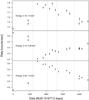 |
Fig. 1 Observed count rates of RX J0720.4−3125 in the energy ranges 0.16−1.6 keV, 0.16−0.38 keV, and 0.38−1.6 keV in different XMM-Newton EPIC-pn full frame mode observations. |
3. Data analysis
To extract spin-phase-resolved spectra, one has to determine the rotational phase of each registered photon, meaning that an accurate estimate of the most probable value of the spin-period is required for each epoch. In the case of RX J0720.4−3125, apart from the clear variation detected in the spectrum, a significant variation of the spin-period has also been reported. A number of published papers are devoted to the timing analysis and behavior of spectral variations of this enigmatic object (Cropper et al. 2001, 2004; van Kerkwijk et al. 2007; Hohle et al. 2009). To explain significant phase residuals from a steady spin-down model, different interpretations have been suggested; free precession and glitch possibilities are the most-debated (see, e.g., Hohle et al. 2009, 2012a, possible glitch (Δν ~ 4.1(12) nHz at MJD = 52 866 ± 73 d)). However, sometimes an unambiguous identification of the true spin-period of a spinning compact star, for which the pulsed emission is dominated by emitting areas that have slightly different physical characteristics in comparison to the other parts of the surface or atmosphere such as around the magnetic poles, is very difficult from a simple analysis of a periodogram (Buccheri et al. 1983; Ögelman & van den Heuvel 1989)2, meaning by assigning the frequency corresponding to the most significant peak in a periodogram to the true rotational period.
The problem is that, the genuine spin frequency in a periodogram highly depends on the unknown true light curve shape, such as single-, double-, or multiple-peaked profile. This in turn depends on the physical characteristics of the emitting areas, such as temperatures, sizes, and locations, meaning the ratios and locations of the maxima and minima in a light curve, and the viewing geometry, such as the angles between rotation, magnetic axes, line of sight, and gravitationa redshift etc. (for example see Poutanen & Beloborodov 2006).
On the other hand, it is clear that if there is a periodic signal in the dataset with frequency ν, then there is also a less significant signal at 0.5ν. Therefore, the most significant peak in the periodogram unequivocally corresponds to the genuine spin frequency for a single-peaked light curve shape. The situation is not simple for the case of a signal from a double- or multiple-peaked light curve shape. In this case, depending on the parameters mentioned above, the periodogram can be identical to a single-peaked one. Moreover, the dependence of an applied statistic such as  (see Appendix A) from a trial frequency will show a highly significant detection only at twice the true spin frequency, 2ν, if the two emitting areas have identical physical characteristics and favorable viewing geometry such as the orthogonal rotator ( see expression for
  and Fig. 2 in Hambaryan et al. 2015).
These arguments motivated us to perform a complete X-ray timing re-analysis of the observational datasets of RX J0720.4−3125 for the identification of the true pulsation period by using a more advanced analysis, such as a Bayesian analysis of the search, estimate, and testing of the hypothesis following (Gregory & Loredo 1992, hereafter GL). We were also motivated to explore some effects, such as folding into other possible periods, as well half of the frequency of the most significant peak in the periodogram, and checking of the presence of possible asymmetries in the folded light curves over time and various energy ranges, meaning peak-to-peak and minimum-to-minimum ratios and phase differences (for details of methodical concerns, see Hambaryan et al. 2015). Moreover, to solve this challenging problem we perform a study of the distribution of the spin-phases that result from the folding of the photon arrival times into the various frequencies mentioned above (see Appendix A).
3.1. X-ray timing analysis
First of all, for each pointed observation (Table 1), we used the cleaned photon arrival times (see Sect. 2) to apply the test for periodicity detection in the frequency range of 0.05−0.5 Hz in the broad energy band (0.16−1.6 keV). We note that this range includes, as reported in the literature, the spin frequency 0.119 Hz of RX J0720.4−3125 and the second harmonic and subharmonic frequencies. As already mentioned in Sect. 3, the periodograms reveal a very significant peak at the frequency 0.119 Hz. Apart from that they also show a less significant second peak at the frequency of 0.0596 Hz, in other words close to half the frequency of the most significant peak. In Fig. 2, we present the statistic periodogram of two observations (Obsids: 0124100101 and 0164560501, see Table 1 and Fig. 1) that corresponds to the first and the brightest phase of RX J0720.4−3125 in the long-term light curve.
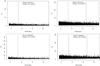 |
Fig. 2
|


If we apply the H-test developed by de Jager et al. (1989), de Jager & Büsching (2010)3 to the datasets, we identify a second peak in all pointed observations of RX J0720.4−3125 in different energy bands. Moreover, for some energy bands, the pointed observations show a more significant peak corresponding to 0.0596 Hz instead of 0.119 Hz.
These results led us to consider the frequency 0.0596 Hz as the most probable true spin-period of RX J0720.4−3125 and to perform a detailed analysis of the light curve shapes in different energy bands. For this purpose, we applied the GL method, together with and H-statistics, to the different datasets in various energy bands for the frequency ranges 0.05−0.07 Hz and 0.10−0.14 Hz separately. In general, the GL method first tests if a constant, variable, or periodic signal is present in a dataset, given photon arrival times of events or a binned dataset obeying Poissonian counting statistics, when we have no specific prior information about the shape of the signal.
In the GL method, periodic models are represented by a signal of folded photon-arrival times into trial frequencies with a light curve shape that is a stepwise function with m phase bins per period plus a noise contribution. With this kind of a model we are able to approximate a phase-folded light curve of any shape. Hypotheses for detecting periodic signals represent a class of stepwise, periodic models with the following parameters: trial period, phase, noise parameter, and number of bins (m). The most probable model parameters are then estimated by marginalization of the posterior probability over the prior specified range of each parameter. In Bayesian statistics, posterior probability contains a term that penalizes complex models unless there is no significant evidence to support that hypothesis. Therefore we calculate the posterior probability by marginalizing over a range of models corresponding to a prior range of number of phase bins, m, from two to twenty. For all cases that have strong support for the presence of a periodic signal, using posterior probability density functions we estimated the most probable values and uncertainties of all parameters, meaning the frequency4, phase, and the most probable number of phase bins of a periodic signal. Results are presented in Table 2 and Figs. 3 and 4. Using these results, we created phase-folded light curves for all observations of RX J0720.4−3125 in three different energy bands: soft, 0.16−0.38 keV; hard, 0.38−1.6 keV; and broad, 0.16−1.6 keV, Figs. B.1−B.4).
Results of the application of the GL method in the frequency range of 0.05−0.07 Hz for the broad energy band of 0.16−1.60 keV.
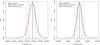 |
Fig. 3 Estimated most probable spin frequencies of RX J0720.4−3125 (for details, see text and Table 2) obtained by application of the GL method for periodicity searching in the broad energy band for ObsIds 0124100101 and 0164560501 (XMM-Newton EPIC-pn Full Frame mode). The highest posterior density (HPD) intervals, 68% and 95%, are determined as a probabilistic region around a posterior mode and depicted as vertical dashed lines in black and red, respectively. |
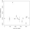 |
Fig. 4 Spin frequency history of RX J0720.4−3125 (for details, see text and Table 2) obtained by application of the GL method for periodicity searching in the broad energy band for different XMM-Newton EPIC-pn full frame mode observations. |
In addition, we constructed combined phase-folded light curves (Figs. 5, B.5) for all observations and different data groups (see Sect. 3.2) that clearly show the dependence of the double-peak light curve profile upon the energy band (cf., e.g., Hambaryan et al. 2011). Indeed, the relative strength of the modulation5 for all the combined data groups are 0.07 ± 0.02, 0.05 ± 0.02, 0.07 ± 0.02, and 0.12 ± 0.04 in the energy bands of 0.16−0.5 keV, 0.5−0.6 keV, 0.6−0.7 keV, 0.7−2.0 keV, respectively. Thus, the X-ray phase-folded light curves of RX J0720.4−3125 (cf., RBS1223 with the spin-period of 10.31 s, Hambaryan et al. 2011) have a markedly double-humped shape with different ratios of maxima in different spectral bands. Moreover, they can be parameterized with a mixed von Mises distribution (see Appendix A, Fig. A.1, Table A.1), in other words with a double-peaked light curve profile that shows a dependence of the estimated parameters, such as mean directions, concentrations, and proportion upon the energy band and indicates that radiation emerges from at least two emitting areas. These spin-phase-folded light curves and the estimated parameters from the distribution of phases may serve as rough estimates of the viewing geometry and physical characteristics of the emitting areas (see below).
Simultaneous fitting results of combined, spin-phase averaged X-ray spectra of RX J0720.4−3125 with a spectral model of an absorbed blackbody with and without a Gaussian absorption line (in XSPEC tbabs*bbodyrad*gabs).
3.2. Rotational phase-resolved X-ray spectral analysis
To create high signal-to-noise (S/N) ratio spin-phase-resolved spectra of RX J0720.4−3125 we coadded spectra for some sequential pointed observations where it shows approximately similar brightness in the broad energy band (0.16−1.6 keV). Namely, the total observational interval that spanned almost 12.5 yr was divided into five groups (see, Fig. 1 vertical dashed-lines). The second group represents the brightest phase of RX J0720.4−3125 in the hard energy band.
Firstly, we simultaneously fit the phase-averaged, high S/N ratio spectral data collected from different observations (Table 1), which were greater than thirty with each spectral bin containing at least 1000 counts. We used a combination of an absorbed blackbody and a Gaussian absorption line, a multiplicative component, in the model (in XSPEC tbabs*bbodyrad*gabs, see Fig. 6 and Table 3). During the fitting, the interstellar absorption and the Gaussian line energy were kept linked or free (see, Table 3), whereas other parameters such as blackbody temperature, Gaussian width, and normalizations were left free for different data groups. We note that if the linked parameters were also left free, the fitting results remained almost unchanged. It is also worthwhile to note that these spectra cannot be fit with the model of fixed parameters of the absorption line feature at the pre-brightening phase.
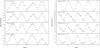 |
Fig. 5 Combined phase-folded light curves for RBS 1223 (left panel Hambaryan et al. 2011) and RX J0720.4−3125 (right panel) in different energy bands: 0.16−0.5 keV, 0.5−0.6 keV, 0.6−0.7 keV, and 0.7−2.0 keV. |
Secondly, we extracted high S/N ratio spectral data, which were greater than ten with each spectral bin containing at least 100 counts, corresponding to the eight rotational phase bins, meaning the maxima, minima, and intermediate stages, of the double-peaked pulse profile and collected from different observations (see, Figs. 5, B.5). These forty spectra for the five data groups were subject to simultaneous fitting with a number of highly magnetized INS surface/atmosphere models developed by us (Suleimanov et al. 2010) and implemented into the X-ray spectral fitting package XSPEC (Hambaryan et al. 2011). They are based on various local surface models and compute rotational-phase-dependent integral emergent spectra of INS using analytical approximations. The basic model includes temperature and magnetic field distributions over the INS surface, viewing geometry, and gravitational redshift. Three local radiating surface models are also considered: a naked condensed iron surface with a partially ionized hydrogen model atmosphere that is either semi-infinite or finite on top of the condensed surface. To compute an integral spectrum, the model uses an analytical expression for the local spectra, an emitting condensed iron surface, and a diluted blackbody spectrum transmitted through the thin magnetized atmosphere with an absorption feature. The center of the line depends on the local magnetic field strength, representing either the ion cyclotron line for completely ionized iron and/or the blend of the proton-cyclotron and bound-bound atomic transitions in neutral hydrogen. In the latter case, the center of the line is parameterized by half of a Gaussian line with the following parameters: Eline, optical depths  , and the widths σline (for details and further references, see Suleimanov et al. 2010; Hambaryan et al. 2011).
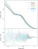 |
Fig. 6 Combined spin-phase averaged spectra and simultaneously-fit spectral model of an absorbed blackbody and a Gaussian absorption line for RX J0720.4−3125. We note that the observed flux is almost the same before and after the variation at E0 ~ 0.38 keV. |
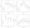 |
Fig. 7 Box-plots of the MCMC fit parameters kTp1,kTp2 (upper panel) and τ,σ (bottom panel) in the energy band of 0.16−2.0 keV of RX J0720.4−3125 for different groups combined from multi-epoch pointed XMM-Newton EPIC-pn observations with spectral model of a condensed iron surface and a partially ionized hydrogen atmosphere (for details see text and Table 4). |
Given the large number of free parameters in the model, we performed a preliminary analysis to get rough estimates, or constraints, on some of them. From the observed double-peaked profile light curve shape in different energy bands (see, right panel Fig. 5 and Fig. B.5), it was already clear that the two emitting areas have slightly different spectral and geometrical characteristics, such as the relatively cooler one has a larger size. Secondly, some constraints, in other words initial values for the fitting, on magnetic field strengths at the poles may be used on the base of the period and its derivative values6, assuming magnetic dipole braking as a main mechanism of the spin-down of RX J0720.4−3125 (see, e.g., Hohle et al. 2012b; Hambaryan & Neuhäuser 2016). Moreover, from the peak-to-peak separation and the ratio of the minima in this double-humped light curve, we may locate the cooler one at an offset angle with respect to the magnetic axis and azimuth (Schwope et al. 2005).
Having these general constraints on temperatures and magnetic field strengths at the poles, we simulated a large number of photon spectra, absorbed blackbody with Gaussian absorption line, folded with the response of the XMM-Newton EPIC-pn camera with the same observing mode of RX J0720.4−3125. We also included the interstellar absorption (for parameters see Table 3), and used a characteristic magnetic field strength of B ~ 3.0 × 10¹³ Gauss. The predicted phase-folded light curves in four spectral ranges, 0.16−0.5 keV, 0.5−0.6 keV, 0.6−0.7 keV, and 0.7−2.0 keV, were cross-correlated with the observed ones (Fig. 5). The predicted curves have a purely dipolar magnetic field configuration that depends on the relative orientation between the magnetic axis, the rotation axis, the observer line of sight, and the gravitational redshift (see upper left panel of Fig. A.1), and were normalized to the mean of the brightness. We inferred some constraints on the parameters from their unimodal distributions when cross-correlation coefficients exceeded 0.9 in the mentioned four energy bands simultaneously. We then used the parameters as the initial input values and as the lower and upper bounds for fitting purposes. For example, gravitational redshift cannot exceed 0.3 because it is not possible to obtain the observed relative strength of modulation at larger z due to strong light bending, and the antipodal shift angle must be less than 5° due to the observed phase separation between the two peaks in the light curve. It is also evident that the sum of the inclination angle of the line of sight and magnetic poles relative to the rotational axis are already constrained by the light curve class (see, Poutanen & Beloborodov 2006, class III).
Having the abovementioned crude constraints and input values of the free parameters, we performed fitting with the models implemented in the XSPEC package of all the combined spectra of RX J0720.4−3125 (see Table 1 and Fig. 1) simultaneously, meaning that each of those phase-resolved spectra were considered as a different dataset with fixed spin-phase and with linked parameters to the other datasets.
The model that was fit is presented in Table 4 (see also, upper left panel of Fig. A.1). The model had: a chi-squared fit statistic value of 6070 for 4910 degrees of freedom; a dipolar field configuration with magnetic field strengths at the poles of Bp1 ≈ Bp2 ~ (0.3 ± 0.02) × 1014 G; an orthogonal rotator with an angle between the magnetic and the rotation axis of θ = (89 ± 5)°; an inclination angle with an angle between the rotation axis and the observer line of sight of i = (42 ± 3)°; and a shift angle of κ ~ 0°. To assess the degree of uniqueness and to estimate confidence intervals of the determined parameters, we additionally performed a Markov chain Monte Carlo (MCMC) fitting as implemented in XSPEC. The parameters of the model that was fit are presented in Table 4 and Fig. 7. In Fig. 8 we present the probability density distributions of the gravitational redshift. We note that independent initial input values of parameters of the MCMC approach converged to the same values in different chains.
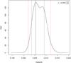 |
Fig. 8 Probability density distributions of gravitational redshift by MCMC fitting with the model of a neutron star with a condensed surface and a partially ionized hydrogen layer above it. The most probable parameter value is indicated by the vertical solid line. Vertical dashed lines indicate the highest probability interval (68% and 95%, for details see text). |
Simultaneous fitting results of combined, spin-phase resolved X-ray spectra of RX J0720.4−3125 using a condensed iron surface and hydrogen atmosphere model.
4. Discussion
Our comprehensive X-ray timing analysis of RX J0720.4−3125, based on the XMM-Newton EPIC-pn long-term pointed observations, shows that the most probable and plausible spin frequency of this INS is 0.0596 Hz, instead of 0.119 Hz as reported in the literature. The phase-folded light curves of this period show a markedly double-peaked shape, which can be formally parameterized with a mixed von Mises distribution that contains significantly different components, such as concentration and mixing proportion parameters (see Appendix A).
We had seen a similar picture with RBS 1223, another INS. The pulsation discovery paper reports on a spin-period 5.16 s (Hambaryan et al. 2002); however, a more detailed study shows that true period is 10.31 s (Haberl et al. 2003; Haberl 2004; Schwope et al. 2005, 2007). Namely, this period with its double-peaked profile is suggested by the presence of a second peak with lower significance in the power spectrum (Haberl 2004). Further analysis of light curves in different energy bands and phase-resolved spectroscopic study (Schwope et al. 2007; Hambaryan et al. 2011) provides additional confirmation of the plausibility of the model of RBS 1223 in which emergent emission is dominated by two emitting areas with slightly different parameters. Yet another case, Speagle et al. (2011), notes that without the radio period, they might have actually identified the pulse period of PSR J0726 as half of the true value. Cropper et al. (2001) performed spin pulse profile analysis of RX J0720.4−3125 based on earlier XMM-Newton observations and folded photon-arrival times that are twice the detected period, via Fourier periodogram, that produces a double-humped light curve with different count rates at the different peaks. However, having no indication of subharmonics in the periodogram, they do not really consider twice the period as correct. Another possible indication of the double-peaked light curve shape of RX J0720.4−3125 may be the non-sinusoidal light curve shape and the reported phase lag in different energy bands (Haberl et al. 2006; Hohle et al. 2009). Indeed, slightly different effective temperatures and sizes of two emitting areas at the magnetic poles that are not located exactly in podal and antipodal directions may cause this kind of a lag, if the photon arrival times fold into phases with half of the value of the genuine spin-period (see Fig. A.1).
The combined phase-resolved spectra of RX J0720.4−3125 can also be fit by emergent radiation of a spectral model of an iron condensed surface with a partially ionized hydrogen atmosphere above it. Formally they can also be fit by a blackbody spectrum with a proton-cyclotron absorption Gaussian line and a peaked angular distribution of the emergent radiation that is typical for an electron scattering atmosphere. In both cases, two emitting areas with slightly different characteristics are required (see Table 4). It is worth noting that the resulting fit parameters are very similar for different spectral models, and were also confirmed by an MCMC approach with different input parameters.
However, we believe that the emission properties that are due to the condensed surface model with a partially ionized, optically thin hydrogen layer above it, including vacuum polarization effects, are more physically motivated. Moreover, semi-infinite atmospheres have somewhat fan-beamed emergent radiation (see Suleimanov et al. 2010; Hambaryan et al. 2011, and references therein) and it seems impossible to combine a proton-cyclotron line with a pencil-beamed emergent radiation.
Emission spectra based on realistic temperature and magnetic field distributions with strongly magnetized hydrogen, or other light element, atmospheres are formally still an alternative7, but they are unphysical because the absorption line is added by hand.
A pure proton-cyclotron absorption line scenario can be excluded owing to the width of the observed absorption spectral feature in the X-ray spectrum of RX J0720.4−3125. Magnetized semi-infinite atmospheres predict too low an equivalent width of the proton-cyclotron line in comparison with the observed one. This result of spectral modelling, meaning the fitting with the condensed surface model with a partially ionized, optically thin hydrogen atmosphere above it, including vacuum polarization effects, suggests a true radius of RX J0720.4−3125 of 13.3 ± 0.5 km for a standard neutron star of 1.4 solar mass, and indicates a stiff equation of state of RX J0720.4−3125 (for similar results, see also Ho et al. 2007; Heinke et al. 2006; Suleimanov & Poutanen 2006; Suleimanov et al. 2011).
Our model fits provide the angles between our line of sight and both the rotation axis and the magnetic field axes, for which we obtain 42 ± 3° and 47 ± 6°, respectively. The direction of motion should be similar to the former angle in case of spin-orbit almost (see, e.g., Ng & Romani 2007, θ < 15°) alignment.
In Tetzlaff et al. (2011), the direction of motion was determined to be 62 ± 9°, by tracing back the motion of RX J0720.4−3125 to its possible birth association Trumpler-10. The direction of motion determined kinematically is thus roughly consistent with an almost-alignment of the spin and orbit.
5. Conclusions
We carried out a complete X-ray timing re-analysis of the multi-epoch observational datasets of RX J0720.4−3125 for an identification of the true spin-period. The genuine spin-period of the isolated neutron star RX J0720.4−3125 is twice of the previously reported value in the literature, 16.78 s instead of 8.39 s, with a markedly double-peaked light curve profile that depends on time and energy.
The observed phase-resolved spectra of the INS RX J0720.4−3125 are satisfactorily fit with slightly different physical and geometrical characteristics of two emitting areas, using the model of a condensed iron surface, with a partially ionized, optically thin hydrogen atmosphere above it, including vacuum polarization effects, and an orthogonal rotator. The fit also suggests the absence of a strong toroidal magnetic field component. Moreover, the determined mass-radius ratio, (M/M⊙)/(R/ km) = 0.105 ± 0.002, suggests a very stiff equation of state of RX J0720.4−3125.
It will be certianly worth doing more work to develop a detailed spectral model (also with quadrupole magnetic field configuration) computation in the near future and apply it to the phase-resolved spectra of other INSs and magnetars, in particular high resolution spectra observed by XMM-Newton and Chandra which possibly have other absorption and emission features (Hambaryan et al. 2009; Potekhin 2010; Hambaryan & Neuhäuser 2016).
High signal-to-noise ratio spectra, for which relative errors in each spectral bin are on the order of a few percent, for different rotational phases can be achieved by combining observations performed at different epochs.
A commonly used statistics in X-ray astronomy is: 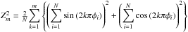 with phases φi at trial frequency. Here,
 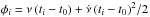 is the phase, ν and
  are the trial frequency and its derivative, ti (i = 1,...,N) are the photon arrival times, and t0 is the epoch of zero phase. We note that
  is a sufficient statistic for detection of sinusoidal signals in comparison to the arrival times, if they are distributed uniformly (obeying constant-rate Poissonian counting statistic, i.e., a periodic component is absent).
The H-test  is a modified
  test that includes higher harmonics and finds an optimal number of them to be included in the search and detection of a periodic signal.
In the GL method, a posterior probability density function is evaluated for any parameter of the model by application of Bayes theorem, e.g., for the trial frequency (ν):
 C and
C and  are the normalization constant and number of ways the binned distribution could have arisen “by chance”. nj(ν,φ) is the number of events falling into the j th of m phase bins given the frequency, ν, and phase, φ. N is the total number of photons (for details, see Gregory & Loredo, 1992, 1993). For its uncertainty, the highest posterior density (HPD) interval is determined as a probabilistic region around a posterior mode or moment, and is similar to a confidence interval in classical statistics.
We have employed the relative strength of modulation
 (1)
instead of the pulsed-fraction PF = (CRmax−CRmin)/(CRmax + CRmin) as an appropriate descriptor of the pulsed emission for complex shape light curves, in which the strengths of variations are independent of the light curve shape, i.e., single or double pulse profile. Here CR is the count-rate. We note that our defined relative strength of the modulation for a single-peaked sinusoidal light curve differs by a factor of 2 /π from the definition of semi-amplitude or pulsed-fraction.
(1)
instead of the pulsed-fraction PF = (CRmax−CRmin)/(CRmax + CRmin) as an appropriate descriptor of the pulsed emission for complex shape light curves, in which the strengths of variations are independent of the light curve shape, i.e., single or double pulse profile. Here CR is the count-rate. We note that our defined relative strength of the modulation for a single-peaked sinusoidal light curve differs by a factor of 2 /π from the definition of semi-amplitude or pulsed-fraction.
We failed in our attempt to fit the combined, phase-averaged spectrum of RX J0720.4−3125 by a partially ionized, strongly magnetized hydrogen or a mid-Z element plasma model (XSPEC nsmax, Mori & Ho 2007; Ho et al. 2008), or two spots or purely condensed iron surface models. It is worth noting that an acceptable fit is obtained by the nsmax model with an additional, multiplicative Gaussian absorption line component (modelgabs).
Acknowledgments
V.H., V.S., and R.N. acknowledge support by the German National Science Foundation (Deutsche Forschungsgemeinschaft, DFG) through project C7 of SFB/TR 7 “Gravitationswellenastronomie”.
References
- Borghese, A., Rea, N., Coti Zelati, F., Tiengo, A., & Turolla, R. 2015, ApJ, 807, L20 [NASA ADS] [CrossRef] [Google Scholar]
- Buccheri, R., Bennett, K., Bignami, G. F., et al. 1983, A&A, 128, 245 [NASA ADS] [Google Scholar]
- Connors, A. 1997, in Data Analysis in Astronomy, eds. V. Di Gesu, M. J. B. Duff, A. Heck, M. C. Maccarone, L. Scarsi, & H. U. Zimmerman, 251 [Google Scholar]
- Cropper, M., Zane, S., Ramsay, G., Haberl, F., & Motch, C. 2001, A&A, 365, L302 [NASA ADS] [CrossRef] [EDP Sciences] [Google Scholar]
- Cropper, M., Haberl, F., Zane, S., & Zavlin, V. E. 2004, MNRAS, 351, 1099 [NASA ADS] [CrossRef] [Google Scholar]
- de Jager, O. C., & Büsching, I. 2010, A&A, 517, L9 [NASA ADS] [CrossRef] [EDP Sciences] [Google Scholar]
- de Jager, O. C., Raubenheimer, B. C., & Swanepoel, J. W. H. 1989, A&A, 221, 180 [NASA ADS] [Google Scholar]
- de Vries, C. P., Vink, J., Méndez, M., & Verbunt, F. 2004, A&A, 415, L31 [NASA ADS] [CrossRef] [EDP Sciences] [Google Scholar]
- Gregory, P. C., & Loredo, T. J. 1992, ApJ, 398, 146 [NASA ADS] [CrossRef] [Google Scholar]
- Haberl, F. 2004, Adv. Space Res., 33, 638 [NASA ADS] [CrossRef] [Google Scholar]
- Haberl, F. 2007, Ap&SS, 308, 181 [NASA ADS] [CrossRef] [Google Scholar]
- Haberl, F., Schwope, A. D., Hambaryan, V., Hasinger, G., & Motch, C. 2003, A&A, 403, L19 [NASA ADS] [CrossRef] [EDP Sciences] [Google Scholar]
- Haberl, F., Zavlin, V. E., Trümper, J., & Burwitz, V. 2004, A&A, 419, 1077 [NASA ADS] [CrossRef] [EDP Sciences] [Google Scholar]
- Haberl, F., Turolla, R., de Vries, C. P., et al. 2006, A&A, 451, L17 [NASA ADS] [CrossRef] [EDP Sciences] [Google Scholar]
- Hambaryan, V., & Neuhäuser, R. 2016, in Non-Stable Universe: Energetic Resources, Activity Phenomena and Evolutionary Processes: Byurakan 2016 in press [Google Scholar]
- Hambaryan, V., Hasinger, G., Schwope, A. D., & Schulz, N. S. 2002, A&A, 381, 98 [NASA ADS] [CrossRef] [EDP Sciences] [Google Scholar]
- Hambaryan, V., Neuhäuser, R., Haberl, F., Hohle, M. M., & Schwope, A. D. 2009, A&A, 497, L9 [NASA ADS] [CrossRef] [EDP Sciences] [Google Scholar]
- Hambaryan, V., Suleimanov, V., Schwope, A. D., et al. 2011, A&A, 534, A74 [NASA ADS] [CrossRef] [EDP Sciences] [Google Scholar]
- Hambaryan, V., Neuhäuser, R., Suleimanov, V., & Werner, K. 2014, J. Phys. Conf. Ser., 496, 012015 [Google Scholar]
- Hambaryan, V., Wagner, D., Schmidt, J. G., Hohle, M. M., & Neuhäuser, R. 2015, Astron. Nachr., 336, 545 [NASA ADS] [CrossRef] [Google Scholar]
- Heinke, C. O., Rybicki, G. B., Narayan, R., & Grindlay, J. E. 2006, ApJ, 644, 1090 [NASA ADS] [CrossRef] [Google Scholar]
- Ho, W. C. G., Kaplan, D. L., Chang, P., van Adelsberg, M., & Potekhin, A. Y. 2007, MNRAS, 375, 821 [NASA ADS] [CrossRef] [Google Scholar]
- Ho, W. C. G., Potekhin, A. Y., & Chabrier, G. 2008, ApJS, 178, 102 [NASA ADS] [CrossRef] [Google Scholar]
- Hohle, M. M., Haberl, F., Vink, J., et al. 2009, A&A, 498, 811 [NASA ADS] [CrossRef] [EDP Sciences] [Google Scholar]
- Hohle, M. M., Haberl, F., Vink, J., de Vries, C. P., & Neuhäuser, R. 2012a, MNRAS, 419, 1525 [NASA ADS] [CrossRef] [Google Scholar]
- Hohle, M. M., Haberl, F., Vink, J., et al. 2012b, MNRAS, 423, 1194 [NASA ADS] [CrossRef] [Google Scholar]
- Mardia, K., & Jupp, P. 2009, Directional Statistics, Wiley Series in Probability and Statistics (Wiley) [Google Scholar]
- Mardia, K. V., Taylor, C. C., & Subramaniam, G. K. 2007, Biometrics, 63, 505 [CrossRef] [Google Scholar]
- Mardia, K. V., Hughes, G., Taylor, C. C., & Singh, H. 2008, Can. J. Stat., 36, 99 [CrossRef] [Google Scholar]
- Mendez, M., de Vries, C. P., Vink, J., & Verbunt, F. 2004, in 35th COSPAR Scientific Assembly, ed. J.-P. Paillé, COSPAR Meeting, 35, 2075 [Google Scholar]
- Mereghetti, S. 2008, A&ARv, 15, 225 [NASA ADS] [CrossRef] [Google Scholar]
- Mori, K., & Ho, W. C. G. 2007, MNRAS, 377, 905 [NASA ADS] [CrossRef] [Google Scholar]
- Motch, C., Zavlin, V. E., & Haberl, F. 2003, A&A, 408, 323 [NASA ADS] [CrossRef] [EDP Sciences] [Google Scholar]
- Ng, C.-Y., & Romani, R. W. 2007, ApJ, 660, 1357 [NASA ADS] [CrossRef] [Google Scholar]
- Ögelman, H., & van den Heuvel, E. P. J. 1989, Timing Neutron Stars, NATO Advanced Science Institutes (ASI) Series C (Dordrecht: Kluwer), Vol. 262, [Google Scholar]
- Pérez-Azorín, J. F., Pons, J. A., Miralles, J. A., & Miniutti, G. 2006, A&A, 459, 175 [NASA ADS] [CrossRef] [EDP Sciences] [Google Scholar]
- Potekhin, A. Y. 2010, A&A, 518, A24 [NASA ADS] [CrossRef] [EDP Sciences] [Google Scholar]
- Poutanen, J., & Beloborodov, A. M. 2006, MNRAS, 373, 836 [NASA ADS] [CrossRef] [Google Scholar]
- Schwope, A. D., Hambaryan, V., Haberl, F., & Motch, C. 2005, A&A, 441, 597 [NASA ADS] [CrossRef] [EDP Sciences] [Google Scholar]
- Schwope, A. D., Hambaryan, V., Haberl, F., & Motch, C. 2007, Ap&SS, 308, 619 [NASA ADS] [CrossRef] [Google Scholar]
- Speagle, J. S., Kaplan, D. L., & van Kerkwijk, M. H. 2011, ApJ, 743, 183 [NASA ADS] [CrossRef] [Google Scholar]
- Strüder, L., Briel, U., Dennerl, K., et al. 2001, A&A, 365, L18 [NASA ADS] [CrossRef] [EDP Sciences] [Google Scholar]
- Suleimanov, V., & Poutanen, J. 2006, MNRAS, 369, 2036 [NASA ADS] [CrossRef] [Google Scholar]
- Suleimanov, V., Hambaryan, V., Potekhin, A. Y., et al. 2010, A&A, 522, A111 [NASA ADS] [CrossRef] [EDP Sciences] [Google Scholar]
- Suleimanov, V., Poutanen, J., Revnivtsev, M., & Werner, K. 2011, ApJ, 742, 122 [NASA ADS] [CrossRef] [Google Scholar]
- Tetzlaff, N., Eisenbeiss, T., Neuhäuser, R., & Hohle, M. M. 2011, MNRAS, 417, 617 [NASA ADS] [CrossRef] [Google Scholar]
- Turolla, R. 2009, in Neutron Stars and Pulsars, ed. W. Becker, Astrophys. Space Sci. Libr., 357, 141 [Google Scholar]
- van Kerkwijk, M. H., Kaplan, D. L., Pavlov, G. G., & Mori, K. 2007, ApJ, 659, L149 [NASA ADS] [CrossRef] [Google Scholar]
- Viganò, D., Perna, R., Rea, N., & Pons, J. A. 2014, MNRAS, 443, 31 [NASA ADS] [CrossRef] [Google Scholar]
- Zane, S., & Turolla, R. 2006, MNRAS, 366, 727 [NASA ADS] [CrossRef] [Google Scholar]
- Zavlin, V. E., Pavlov, G. G., Shibanov, Y. A., & Ventura, J. 1995, A&A, 297, 441 [NASA ADS] [Google Scholar]
Appendix A: True spin-period of RX J0720.4−3125
Results of the fitting of spin-phases with a two-component mixed von Mises distribution.
Most of the methods for the search and detection of a periodicity in X-ray astronomy are based on the analysis of the distribution of the phases ( ), which are the result of folding photon arrival times (ti (i = 1,...,N) with a trial frequency (ν) and its derivative () for the epoch of zero phase (t0, e.g., , H-test, the GL method, etc.). This procedure transforms the time variable to phases distributed on a circle.
To disentangle between a single- or multiple-peaked profile of a light curve shape the phases have to be analyzed statistically. For this purpose, commonly-used circular distributions are the von Mises distribution, the wrapped normal distribution, and the wrapped Cauchy distribution, etc. The von Mises distribution ( ) has two parameters: the mean direction and concentration of the data distributed on a circle (I0(κ) is the modified Bessel function of order 0).
For demonstration purposes, in Fig. A.1 we show a sample of the light curve shape that is modeled by an exponentiated Fourier series or generalized von Mises distribution (Connors 1997) for two components (![Mathematical equation: \hbox{$r(t_{i})\propto {\rm e}^{\sum_{j=1}^{2}{[-\kappa_j\cos(\frac{2\pi t_{i}}{P}+\varphi_j)]}}$}](/articles/aa/full_html/2017/05/aa30368-16/aa30368-16-eq150.png) , with the phases ϕ1,2 of photon arrival times (ti,i = 1,N) of a periodic signal with the period of P). The distribution of phases, indicated using a rose diagram that is a circular histogram plot of a mixed two von Mises distribution (Mardia & Jupp 2009; Connors 1997), mean that
, with the phases ϕ1,2 of photon arrival times (ti,i = 1,N) of a periodic signal with the period of P). The distribution of phases, indicated using a rose diagram that is a circular histogram plot of a mixed two von Mises distribution (Mardia & Jupp 2009; Connors 1997), mean that  ,where μ1,μ2 are the mean directions of the phases, κ1,κ2 are concentrations, and p is a mixing proportion. These parameters determine the locations, peakedness, and relative contribution of each component of a double-profile light curve, meaning that they are expressing the effective temperatures and sizes of the dominating areas from which the emergent radiation arises.
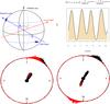 |
Fig. A.1 Upper panel: example of a simulated double-peaked light curve |
![Mathematical equation: \hbox{$r(t)\propto {\rm e}^{\sum_{j=1}^{2}[f_j\cos(\frac{2\pi t}{P}+\varphi_j)]} $}](/articles/aa/full_html/2017/05/aa30368-16/aa30368-16-eq157.png)
To fit the double-peaked light curve profile we coded an expectation-maximization algorithm, an iterative approach to find the maximum of the likelihood applied to a mixture models (see, e.g., Mardia et al. 2007, 2008), that is used to model the rotational phases of all registered photons (column N in Table A.1) as a mixture of a two component von Mises distribution. The results of the fit are presented in Table A.1, where for the estimation of uncertainties, an additional, bootstrap algorithm was implemented and applied. We generate a bootstrap sample of thirty datasets for each data group by randomly sampling from original spin-phases without replacement. Each of these bootstrap datasets were fit with a mixture of a two component von Mises distribution. The standard deviations of the derived parameters are accepted as an uncertainty measure.
An application of the so-called one sample t-test to the difference of the locations of the peaks (column μ1/μ2, Table A.1, or two-sample paired t-test to the μ1 and μ2) of the phase-folded light curve for the double-peaked profile is consistently approximately π, regardless of the energy band. Hence, the null hypothesis on the equality of the ratio of the mean directions of 0.5 (i.e., podal and antipodal directions) is accepted. In contrary, for the parameters of concentration and proportion, κ1/κ2 and p, the null hypothesis is rejected, κ1 and κ2 are nonidentical populations and thep mean value is not equal to 0.5 (see, Table A.1). We arrive to similar conclusions by an application of a non-parametric Wilcoxon test.
Appendix B: Phase-folded light curves
Here (Fig. B.1), we present rotational phase-folded light curves for all pointed observations of RX J0720.4−3125 performed by XMM-Newton EPIC-pn in different energy bands, 0.16−0.38 keV, 0.38−1.6 keV, and 0.16−1.6 keV, with spin frequencies (Table 2), zero-phases derived by an application of the GL method, and using twenty phase bins. All double-peaked profile light curves are normalized to the mean count rate of the pointed observations in the corresponding energy band.
 |
Fig. B.1 Phase-folded light curves in different energy bands, 0.16−0.38 keV, 0.38−1.6 keV, and 0.16−1.6 keV left, middle, and right panels, accordingly, of RX J0720.4−3125 for pointed XMM-Newton EPIC-pn observations 0124100101, 0156960201, 0156960401, and 0164560501. |
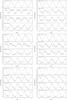 |
Fig. B.5 Combined phase-folded light curves of different data groups GR I, II, III (left panel, from top to bottom), IV, V and all datasets (right panel) in different energy bands, 0.16−0.50 keV, 0.50−0.60 keV, 0.60−0.70 keV, and 0.70−2.0 keV. |
Appendix C: Phase-resolved spectra with MCMC
As already mentioned, to assess the degree of uniqueness and to estimate the confidence intervals of the determined parameters for the model of an emitting condensed iron surface with a partially ionized hydrogen model atmosphere, (see, Sect. 3.2), we additionally performed a Markov chain Monte Carlo (MCMC) fitting using the Goodman-Weare chain-generating algorithm, which is the default in XSPEC. The results for the basic parameters of the fitted model for two data groups I and II are presented as a matrix plot (see, Fig. C.1).
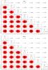 |
Fig. C.1 Fit spectral model parameters, kept free for all data groups, and MCMC verification results for data groups before the variation (GR I, upper panel), and at the brightest stage (GR II, lower panel) of RX J0720.4−3125. Derived probability density functions of the basic parameters of the fit model are presented in the diagonal. The lower triangular part depicts samplings from the posteriors of two parameters, whereas the upper one depicts their mutual correlations. |
All Tables
Results of the application of the GL method in the frequency range of 0.05−0.07 Hz for the broad energy band of 0.16−1.60 keV.
Simultaneous fitting results of combined, spin-phase averaged X-ray spectra of RX J0720.4−3125 with a spectral model of an absorbed blackbody with and without a Gaussian absorption line (in XSPEC tbabs*bbodyrad*gabs).
Simultaneous fitting results of combined, spin-phase resolved X-ray spectra of RX J0720.4−3125 using a condensed iron surface and hydrogen atmosphere model.
Results of the fitting of spin-phases with a two-component mixed von Mises distribution.
All Figures
|
Fig. 1 Observed count rates of RX J0720.4−3125 in the energy ranges 0.16−1.6 keV, 0.16−0.38 keV, and 0.38−1.6 keV in different XMM-Newton EPIC-pn full frame mode observations. |
| In the text | |
|
Fig. 2
|
| In the text | |
|
Fig. 3 Estimated most probable spin frequencies of RX J0720.4−3125 (for details, see text and Table 2) obtained by application of the GL method for periodicity searching in the broad energy band for ObsIds 0124100101 and 0164560501 (XMM-Newton EPIC-pn Full Frame mode). The highest posterior density (HPD) intervals, 68% and 95%, are determined as a probabilistic region around a posterior mode and depicted as vertical dashed lines in black and red, respectively. |
| In the text | |
|
Fig. 4 Spin frequency history of RX J0720.4−3125 (for details, see text and Table 2) obtained by application of the GL method for periodicity searching in the broad energy band for different XMM-Newton EPIC-pn full frame mode observations. |
| In the text | |
|
Fig. 5 Combined phase-folded light curves for RBS 1223 (left panel Hambaryan et al. 2011) and RX J0720.4−3125 (right panel) in different energy bands: 0.16−0.5 keV, 0.5−0.6 keV, 0.6−0.7 keV, and 0.7−2.0 keV. |
| In the text | |
|
Fig. 6 Combined spin-phase averaged spectra and simultaneously-fit spectral model of an absorbed blackbody and a Gaussian absorption line for RX J0720.4−3125. We note that the observed flux is almost the same before and after the variation at E0 ~ 0.38 keV. |
| In the text | |
|
Fig. 7 Box-plots of the MCMC fit parameters kTp1,kTp2 (upper panel) and τ,σ (bottom panel) in the energy band of 0.16−2.0 keV of RX J0720.4−3125 for different groups combined from multi-epoch pointed XMM-Newton EPIC-pn observations with spectral model of a condensed iron surface and a partially ionized hydrogen atmosphere (for details see text and Table 4). |
| In the text | |
|
Fig. 8 Probability density distributions of gravitational redshift by MCMC fitting with the model of a neutron star with a condensed surface and a partially ionized hydrogen layer above it. The most probable parameter value is indicated by the vertical solid line. Vertical dashed lines indicate the highest probability interval (68% and 95%, for details see text). |
| In the text | |
|
Fig. A.1 Upper panel: example of a simulated double-peaked light curve |
| In the text | |
|
Fig. B.1 Phase-folded light curves in different energy bands, 0.16−0.38 keV, 0.38−1.6 keV, and 0.16−1.6 keV left, middle, and right panels, accordingly, of RX J0720.4−3125 for pointed XMM-Newton EPIC-pn observations 0124100101, 0156960201, 0156960401, and 0164560501. |
| In the text | |
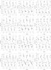 |
Fig. B.2 For ObsIds 0300520201, 0300520301, 0400140301, and 0400140401 (see Fig. B.1). |
| In the text | |
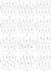 |
Fig. B.3 For ObsIds 0502710201, 0502710201, 0554510101, and 0601170301 (see Fig. B.1). |
| In the text | |
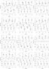 |
Fig. B.4 For ObsIds 0650920101, 0670700201, 0670700301, and 0690070201 (see Fig. B.1). |
| In the text | |
|
Fig. B.5 Combined phase-folded light curves of different data groups GR I, II, III (left panel, from top to bottom), IV, V and all datasets (right panel) in different energy bands, 0.16−0.50 keV, 0.50−0.60 keV, 0.60−0.70 keV, and 0.70−2.0 keV. |
| In the text | |
|
Fig. C.1 Fit spectral model parameters, kept free for all data groups, and MCMC verification results for data groups before the variation (GR I, upper panel), and at the brightest stage (GR II, lower panel) of RX J0720.4−3125. Derived probability density functions of the basic parameters of the fit model are presented in the diagonal. The lower triangular part depicts samplings from the posteriors of two parameters, whereas the upper one depicts their mutual correlations. |
| In the text | |
Current usage metrics show cumulative count of Article Views (full-text article views including HTML views, PDF and ePub downloads, according to the available data) and Abstracts Views on Vision4Press platform.
Data correspond to usage on the plateform after 2015. The current usage metrics is available 48-96 hours after online publication and is updated daily on week days.
Initial download of the metrics may take a while.