| Issue |
A&A
Volume 601, May 2017
|
|
|---|---|---|
| Article Number | A28 | |
| Number of page(s) | 10 | |
| Section | Extragalactic astronomy | |
| DOI | https://doi.org/10.1051/0004-6361/201630227 | |
| Published online | 24 April 2017 | |
The globular cluster system of NGC 1316⋆
IV. Nature of the star cluster complex SH2
1 Departamento de Astronomía, Universidad de Concepción, Concepción, Chile
e-mail: This email address is being protected from spambots. You need JavaScript enabled to view it.
2 European Southern Observatory, Karl-Schwarzschild-Str. 2, 85748 Garching, Germany
3 Instituto de Astrofísica, Pontificia Universidad Católica de Chile, Av. Vicuña Mackenna 4860, 7820436 Macul, Santiago, Chile
4 Institute for Astronomy, University of Hawaii, 2680 Woodlawn Drive, Honolulu, HI 96822, USA
5 Departamento de Ciencias Físicas, Facultad de Ciencias Exactas, Universidad Andres Bello, Fernández Concha 700, 7591538 Las Condes, Chile
6 Max-Planck-Institut für Astronomie, Königstuhl 17, 69117 Heidelberg, Germany
Received: 9 December 2016
Accepted: 14 February 2017
Abstract
Context. The light of the merger remnant NGC 1316 (Fornax A) is dominated by old and intermediate-age stars. The only sign of current star formation in this big galaxy is the Hii region SH2, an isolated star cluster complex with a ring-like morphology and an estimated age of 0.1 Gyr at a galactocentric distance of about 35 kpc. A nearby intermediate-age globular cluster, surrounded by weak line emission and a few more young star clusters, is kinematically associated. The origin of this complex is enigmatic.
Aims. We want to investigate the nature of this star cluster complex. The nebular emission lines permit a metallicity determination which can discriminate between a dwarf galaxy or other possible precursors.
Methods. We used the Integral Field Unit (IFU) of the VIMOS instrument at the Very Large Telescope of the European Southern Observatory in high dispersion mode to study the morphology, kinematics, and metallicity employing line maps, velocity maps, and line diagnostics of a few characteristic spectra.
Results. The line ratios of different spectra vary, indicating highly structured Hii regions, but define a locus of uniform metallicity. The strong-line diagnostic diagrams and empirical calibrations point to a nearly solar or even super-solar oxygen abundance. The velocity dispersion of the gas is highest in the region offset from the bright clusters. Star formation may be active on a low level. There is evidence for a large-scale disk-like structure in the region of SH2, which would make the similar radial velocity of the nearby globular cluster easier to understand.
Conclusions. The high metallicity does not fit to a dwarf galaxy as progenitor. We favour the scenario of a free-floating gaseous complex having its origin in the merger 2 Gyr ago. Over a long period the densities increased secularly until finally the threshold for star formation was reached. SH2 illustrates how massive star clusters can form outside starbursts and without a considerable field population.
Key words: galaxies: individual: NGC 1316 / galaxies: kinematics and dynamics / galaxies: star clusters: general
Based on observations taken at the European Southern Observatory, Cerro Paranal, Chile, under the programme 082.B-0680, 076.B-0154, 065.N-0166, 065.N-0459.
© ESO, 2017
1. Introduction
NGC 1316 (Fornax A) in the outskirts of the Fornax galaxy cluster is prominent for its abundant signatures of previous galaxy interactions. Starting with the classical work of Schweizer (1980), it has been intensively studied at various wavelengths from X-rays to the radio regime (D’Onofrio et al. 1995; Shaya et al. 1996; Mackie & Fabbiano 1998; Arnaboldi et al. 1998; Longhetti et al. 1998; Kuntschner 2000; Horellou et al. 2001; Goudfrooij et al. 2001b,a; Gómez et al. 2001; Kim & Fabbiano 2003; Bedregal et al. 2006; Nowak et al. 2008; Lanz et al. 2010; Goudfrooij 2012.
Its globular cluster system has been investigated by Richtler et al. (2012a, 2014) and the planetary nebulae population by McNeil-Moylan et al. (2012). More photometric work on the cluster system has been presented by Sesto et al. (2016). Although most of the bright globular clusters show a narrow colour range, compatible with an age of about 2 Gyr, clusters as young as 0.5 Gyr have been found in NGC 1316 (Richtler et al. 2014). However, a corresponding field stellar population of this age has not been identified until now. Even younger clusters are seen at only one place, the Hii region SH2, detected by Schweizer (1980) in the southern outskirts of NGC 1316. Richtler et al. (2012b) presented the first detailed description based on HST/WFPC2 imaging in the F555W and F814W filters and VLT/FORS2 spectroscopy at 5 Å resolution.
This object is a star cluster complex containing about 100 young star clusters within a volume of radius 0.35 kpc. A peculiar feature is another nearby ensemble of blue star clusters with some line emission, grouped around an intermediate-age massive globular cluster of NGC 1316. A tentative interpretation of the nature of SH2 is that of an infalling gas-rich dwarf galaxy, as there are so many traces of previous infall processes through the rich shell system of the galaxy. We are not aware of an obvious comparable object in any other galaxy (but see the remarks on the Ruby Ring in Sect. 7.1), which does not mean that SH2 is too special to provide general insight into the process of star cluster formation. The purpose of the present contribution is to investigate in more detail the line emission, in particular the metallicity of the Hii-gas, which is a key parameter for understanding the formation history of SH2 and which is expected to be low in the case of a dwarf galaxy (e.g. Smith Castelli et al. 2012).
We adopt the supernova type-Ia distance of 17.8 Mpc quoted by Stritzinger et al. (2010), corresponding to a distance modulus of (m−M)0 = 31.25 mag, but see also Cantiello et al. (2013) who quote a larger distance of 20.8 Mpc. One arcsecond corresponds to 86.3 pc at a distance of 17.8 Mpc.
2. Observations and data reduction
We observed the Hii region SH2 roughly centred at RA(J2000): 03h22m38s and Dec(J2000): −37°18′47′′ on October 2012 in service mode with the Integral-Field Unit (IFU) of the VIsible MultiObject Spectrograph (VIMOS, Le Fèvre et al. 2003) mounted on UT3 (Melipal) of the ESO Very Large Telescope in Chile. The high-resolution red (HRR) and blue (HRB) modes were used to cover the wavelength ranges 3900–5335 Å at R ≃ 1700 and 6315–8600 Å at R ≃ 3100, respectively. The field of view was chosen to be 27″ × 27″ with a sampling of 0.67′′ per pixel for both channels. Three individual exposures of 756 s were taken for each channel and accompanied by three flat-field exposures and one arc-lamp exposure. A standard star for flux calibration was also observed for each channel as part of the standard instrument calibration. The seeing during the observations was about 0.8′′.
We performed all data reduction tasks with the independent Py3D data reduction package for fibre-fed IFU spectrographs developed for the data reduction of the Calar Alto Large Integral Field Area (CALIFA) survey data (Husemann et al. 2013). It has been successfully applied to reduce VIMOS IFU data as well (e.g. Husemann et al. 2014) showing superior quality to the standard ESO pipeline. With Py3D we first process the individual exposures performing bias subtraction, cosmic ray detection with PyCosmic (Husemann et al. 2012), fibre tracing and extraction, wavelength calibration, fibre-to-fibre transmission correction, and flux calibration. We also homogenise the highly varying spectral resolution across the VIMOS field to be 2.5 Å in both the HRB and HRR channel. Sky subtraction is done on each exposure by creating a high S/N mean sky spectrum from 200 fibres containing no significant object signal, which is subsequently subtracted from all fibres. Afterwards we combine the individually calibrated exposures to one datacube taking into account differential atmospheric refraction and bad pixels, such as cosmic ray hits or dead CCD pixels.
The world-coordinate system of the data is set by assigning the HST coordinates of the bright star cluster 431-1 of SH2 (Richtler et al. 2014) to the corresponding light weighted centre in the VIMOS data. For convenience we give all coordinates on the IFU in pixels, in the form X:Y for the centres of our spectral extractions (see Sect. 5.2 and Fig. 3), which can be transformed as follows into right ascension (RA) and declination (Dec), both in degrees: 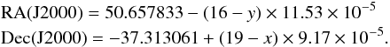
3. Morphology and line maps
3.1. Appearance of the stellar cluster complex
Richtler et al. (2012a) described the appearance of SH2 on the basis of ground-based and HST imaging. The brightest cluster (431-1) has an age of about 0.1 Gyr, based on its colour, and an estimated mass of 1.9 × 10⁵M⊙, if we adopt solar metallicity. The colours indicate a mix of populations with many clusters being even younger, but the extreme crowding prohibits precise measurements. A ring-like structure of the brightest clusters is discernible. At a distance of 12′′ towards the south-west a second assembly of clusters of about the same age exists, but this time the dominant and apparently central object is an intermediate-age globular cluster of NGC 1316. Richtler et al. (2012a) estimated an age of ~2 Gyr and a mass of about 106M⊙. It cannot be excluded that this is a chance projection.
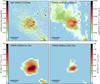 |
Fig. 1 HST image and line maps of SH2. All panels have a size of 27″ × 27″ corresponding to 2.33 × 2.33 kpc2. The 5′′ scale bar corresponds to 432 pc. Upper left panel: F555W HST-WPC2 image, matching the line and continuum maps. Upper right panel: continuum map from the HRB grism spectra, using median values. Lower left panel: Hα flux map from the HRR instrument set-up. Lower right panel: map of the [Oiii]-line at 5007 Å using the HRB set-up. In all frames north is towards the top and east is left. |
3.2. Line maps
A census of line emission regarding extent and intensity in the field of SH2 is provided by Fig. 1. The upper left panel shows an HST-image, where the structure of SH2 is clearly visible (PI: A. Sandage, GO-7504). The upper right panel shows a continuum map, using the median value of the data cube of a given pixel in the HRB mode. Unfortunately, the exposure times are not sufficient to spectroscopically explore the stellar continua. Some of the very faint structure in the upper left quadrant may be flat-field residuals, but the ring of star clusters of SH2 is clearly visible. A faint population between SH2 and the globular cluster 429 is also visible towards the south-west. The colour map of Richtler et al. (2012b) indicates a somewhat redder colour than that of SH2, which is expected if a faint blue population is superimposed on a bright red galaxy background/foreground. At the same time, it is a strong argument that the cluster assembly around 429 still belongs to the SH2 complex.
The lower left panel is an Hα map from the HRR set-up. The dynamical settings of the display make even the faintest structures visible. In particular, it shows that there is no Hα line detected above an S/N > 3 between SH2 and the 429 region. The point of maximum Hα-intensity is a rather well-defined peak and coincides more or less with the most southern point of the “ring”.
In the region of 429, there is a double structure: one peak coincides with the location of 429 itself, the other peak is shifted by about 3′′ to the north-east. A 2 Gyr old star cluster as a source of ionising radiation might appear surprising (see further details in Sect. 7.3).
The lower right panel shows the morphology of the [Oiii]-5007 Å emission with the same absolute flux scaling and also clipping at a threshold of S/N> 3. Its morphology closely resembles that of the Hα emission. The main part of the [Oiii] emission traces the southern part of the ring, peaking roughly at the same location as Hα. The presently ionising (invisible) young stars still seem to follow the overall distribution of the 0.1 Gyr clusters.
4. Velocities and velocity maps
The knowledge of radial velocities in this region so far stems from a few sources: Schweizer (1980) quoted Δvrad ≃ −101 km s-1 as the offset to the systemic velocity of NGC 1316, which is in excellent agreement with the Hi-velocity of SH2 from Horellou et al. (2001) of 1690 km s-1. Richtler et al. (2014) measured radial velocities from medium dispersion VLT/FORS2 spectra for the objects 431 and 429 from the stellar continuum and emission lines. The results are for 429: 1709 ± 12 km s-1 for the emission lines and 1685 ± 20 km s-1 for the stellar continuum, where the quoted uncertainties are internal errors of the used code. The velocity from emission lines for 431 is 1670 ± 20 km s-1.
In Fig. 2 we show the complete kinematics maps, produced by the software PyParadise (Husemann et al. 2016, and in prep.), which is an improved version of Paradise (Walcher et al. 2015). The left panel of Fig. 2 displays the maps of radial velocities, the right panel displays the velocity dispersion. The pixels are not independent because of the seeing, which is slightly larger than the pixel size, but a velocity gradient or rotation is not visible. In the colour scaling of the radial velocity map, the green zone resembles approximately the interior of the ring-like arrangement of star clusters. The intermediate-age globular cluster 429 is offset by about −30 km s-1 with respect to the main body. While the velocity for 431 is in good agreement with that from the FORS spectra, the agreement in the case of 429 is not as good. It is, however, remarkable that 429, as a cluster from the NGC 1316 system with a large velocity dispersion, does not show a larger velocity difference. This could be understood if the entire region were disk-like with only a small extension along the line of sight.
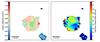 |
Fig. 2 Left panel: radial velocity map of the SH2 region. Neither rotation nor velocity gradients are visible. The globular cluster 429 is offset by about −30 km s-1 from the main body of SH2. The object in the north-western region (also visible in Fig. 1) is a background galaxy without emission lines. The velocity is therefore not valid and the redshift is unknown. Right panel: velocity dispersion map of SH2. Except for the south-western region that is also the zone of the brightest Hα-emission, the dispersion is higher than expected from simple stellar-dynamical considerations. An interesting feature is that the spot with the highest dispersion coincides with the highest [Oiii]-flux intensity (see lower right panel of Fig. 1). |
The velocity dispersion map shows an interesting pattern. It is low in the region of the bright clusters and distinctly higher in the northern part. This spot is also roughly coincident with the secondary maximum of the [Oiii]-emission (see bottom right panel in Fig. 1). Moreover, the line ratios of this region differ from those of the cluster region. We expect a stellar projected velocity dispersion of the order of  , where ℳ is the mass, R a characteristic radius, and G the gravitational constant. The factor β depends on the density slope of the tracer population, the orbit anisotropy, and the mass profile. Under isotropy,
  is a good guess. The dominant mass component is the Hi-mass with about 107M⊙ (Horellou et al. 2001), while the stellar mass has been estimated to be about 106M⊙ (Richtler et al. 2012b). The concentration of the total mass is unknown and not resolved by VLA observations. Setting R = 50 pc and ℳ = 107M⊙, we expect a dispersion of about 17 km s-1, which fits the southern part of the velocity map but not the high values that characterise the [Oiii]-emission. Because stellar dynamics cannot produce a dispersion as high as 40 km s-1, gas dynamics might be a better explanation. Shocks from supernovae and stellar winds might have left their imprints on the interstellar gas. Our data are not appropriate to investigate these possibilities in more detail. Only data with higher S/N to investigate the stellar population itself in combination with higher spectral resolution would give more insight.
5. Spectra and line fluxes
5.1. Fluxes and uncertainties
We measure the line fluxes using the IRAF command splot, in particular the option of fitting and subtracting the underlying stellar spectrum. The treatment of the stellar contribution (lines and continuum) is rather uncritical for the grism HRR because the blue stellar population contributes only very little flux. For example, the Hα flux is not notably affected, while the Hβ-fluxes measured in HRB are higher by about 2% if the stellar spectrum is not subtracted. Because the fainter lines are more strongly affected (by about 5%; this systematic difference disappears largely when line ratios are considered), we measured all fluxes after subtraction of the continua which have been modelled by third-degree polynomials. The fluxes and their uncertainties are given in Tables 1 and 2. The quoted uncertainties are estimated through repeated measurements and do not reflect uncertainties in the flux calibration. For [O iii] and [N ii], only the brighter line of the respective doublet is given. The lines [O iii] 4958 Å and [N ii] 6548 Å are always fainter by a factor of 0.34.
Line fluxes in several selected spectra obtained with HRB.
Line fluxes in several selected spectra obtained with HRR.
5.2. Extraction of some characteristic spectra
Although the substructure within SH2 is not very much larger than the seeing, there are clearly differences in the line strength ratios. To have a sample of characteristic spectra which represents the morphology and the existing line strength ratios, we chose the following (locations are given as x-y-coordinates):
-
1.
global: extraction around 21:21 with a radius of8 pixels. This sums over197 spaxels;
-
2.
spot of brightest Hα-emission: extraction around 17:17 with a radius of 2 pixels. Average over 13 spaxels;
-
3.
globular cluster 429: extraction around 4:5 with a radius of 2 pixels. Average over 13 spaxels;
-
4.
spot of the highest [Oiii]/Hβ ratio: extraction around 25:17 with a radius of 1 pixel. Average over 5 spaxels. This position corresponds to the planetary nebula No. 397 in the catalogue of McNeil-Moylan et al. (2012);
-
5.
spot of the lowest [Oiii]/Hβ ratio: extraction around 22:15 with a radius of 1 pixel. Average over 5 spaxels;
-
6.
star cluster 431: extraction around 20:15 with a radius of 1 pixel. Average over 5 spaxels;
-
7.
north-eastern region of low Hα-emission: extraction around 21:20 with a radius of 2 pixels. Average over 13 spaxels.
Figure 3 shows the locations of the spectra and the approximate sizes of the extraction radii. Figure A.1 displays the total spectrum. We do not show the others because of their similar appearance.
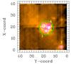 |
Fig. 3 Approximate locations and approximate sizes of the extraction radii of our characteristic spectra. The image is the median of the HRblue data cube. The unusual X-Y-configuration reflects the axes on the original data cube. |
5.3. Hα-flux and star formation rate
We measure the Hα-flux in spectrum 1 that averages over a radius of 8 pixels (see Sect. 5.2). The flux is 60.2 × 10⁻¹⁶ erg/s/cm2 and the luminosity 2.16 × 1038 erg/s. Adopting for the star formation rate the conversion of Panuzzo et al. (2003), SFR/Hα-luminosity = 2.2 × 10-49M⊙/erg, the SFR is 1.5 × 10⁻³M⊙/yr or 2.0 × 10⁻³M⊙/yr/kpc2, much lower than a starburst, and still lower than “normal” star formation rates in normal galaxies (Wuyts et al. 2011). Clearly, there must have been a starburst 0.1 Gyr ago with a much higher Hα-flux of which we now only see the aftermath.
6. Diagnostic graphs
6.1. Models from Dopita et al. (2013)
The precise determination of element abundances in Hii regions normally relies on the determination of electron temperatures, where [Oiii]-4636 Å is the most important line. However, this line is not visible in any of our spectra, which indicates a low temperature and therefore a high metallicity with enhanced cooling capability. This also fits the fact that neutral He-lines are visible. Consequently, we use strong-line diagnostic diagrams to estimate the oxygen abundance of SH2. There is a huge amount of literature on Hii regions and how to use strong-line diagnostic diagrams. We refer to Dopita et al. (2013) and Nicholls et al. (2014) as the primary links with the history of Hii region diagnostics. These authors revisit the physics of Hii regions, using the most recent atomic line parameters, with the motivation that the energy distribution of electrons might be a κ-distribution rather than Boltzmann-Maxwellian (κ = ∞). These works present many diagnostic diagrams using strong lines, of which only a few are useful for us due to the restricted wavelength range. Furthermore, reliable line-ratios are preferably constructed from lines from either HRB or HRR. This leaves us with the diagnostic line ratios [Oiii]/Hβ, [Nii]/Hα, [Sii]/Hα, and [Nii/Sii], which correspond to the diagrams Figs. 9, 10, and 22 of Dopita et al. (2013; in the case of [Nii], we refer to the 6548 Å line, in the case of [Sii] to the sum of the 6715 Å and 6731 Å lines). The [Ariii]-line at 7135 Å is too weak to permit sensible measurements. The line ratios and the locations of our selected spectra in these diagnostic diagrams are shown in Table 3 and in Fig. 4. Their uncertainties are calculated by error propagations of the uncertainties shown in Tables 1 and 2.
Diagnostic line ratios (Cols. 3–7) and results from empirical calibrations (Cols. 8–10).
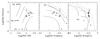 |
Fig. 4 Diagnostic graphs for six selected emission line spectra in SH2 (see Table 3 and Sect. 5.2 for explanation). These spectra are compared to Hii region models from Dopita et al. (2013) with the ionisation parameter log q and four oxygen abundances (0.5 × solar, solar, 2 × solar, and 3 × solar) as parameters. The solid lines are lines of constant oxygen abundance and varying log q. In the left panel, the range of log q values is indicated, and is the same for all panels. The models refer to κ = ∞ (corresponding to a Boltzmann electron distribution). The dotted lines in the middle and right panels separate Hii regions from AGN- and LINER-spectra according to Kewley et al. (2001). All spectra except 25:17 are consistent with a uniform abundance value, although [Oiii]/Hβ varies significantly. The middle and the right graph show the degeneracy for high metallicities that is not present in the left graph. A super-solar oxygen abundance is supported by all three diagnostic graphs. |
The models are taken from Dopita et al. (2013) and use the ionisation parameter log q and the oxygen abundance as parameters. The abundances in solar units are indicated in all panels by the numbers 0.5, 1, 2, 3. The interval of log q values, which is the same for all models, is indicated as well. According to the definition of Dopita et al. (2013), q is the number of ionising photons passing through a unit area divided by the number density of neutral atoms and ions. High q-values are therefore realised when the ionising sources are nearby (planetary nebulae) and/or when the spectrum of ionising photons is harder than that produced by an OB stellar population. Another effect is that for high metallicities, some indices are folded back onto the regime of lower metallicities because the enhanced cooling diminishes the fraction of ionised species with respect to hydrogen. Therefore, there is a limit that line ratios of Hii regions normally do not cross and which can be used to distinguish the line ratios of Hii regions from those of AGNs and LINERs. These limits (which in reality are not very strict) are taken from Kewley et al. (2001), and are indicated for the middle and the right panel by the dotted lines. The log q and abundances are best separated in the left panel, where the lines of constant log q are almost vertical. It is satisfactory that although log q varies, the loci of the spectrum follow a constant abundance line with the exception of 25-17. This is also the case in the middle panel, although there is the above-mentioned degeneracy, in the sense that metal-rich loci cross with the metal-poor ones. The right panel indicates a somewhat lower abundance.
For the interpolation in the tables of Dopita et al. (2013), we use linear expressions in the intervals of interest, which are log q > 7.0 and 1 < z ≤ 3. For the left panel, we obtain (valid only for this selection) ![Mathematical equation: \begin{eqnarray} \begin{split} z &= 1.8 (\pm0.06) +1.8(\pm0.1) \times \log {\rm [NII/SII]} \\ &\quad-1.1(\pm0.03) \times \log {\rm [OIII]}. \end{split} \end{eqnarray}](/articles/aa/full_html/2017/05/aa30227-16/aa30227-16-eq100.png) (1)For the middle panel, we obtain
(1)For the middle panel, we obtain ![Mathematical equation: \begin{eqnarray} \begin{split} z &= 1.44(\pm0.06) -1.42(\pm0.1) \times \log {\rm [SII/H\alpha]} \\ &\quad-1.4(\pm0.08) \times \log {\rm [OIII]}. \end{split} \end{eqnarray}](/articles/aa/full_html/2017/05/aa30227-16/aa30227-16-eq101.png) (2)For the right panel, we adopt the value z = 2.0 with the exception of spectrum 4.
(2)For the right panel, we adopt the value z = 2.0 with the exception of spectrum 4.
Neglecting spectrum 4, the resulting oxygen abundances (in solar units) are 2.44 ± 0.15 for the left panel and 2.31 ± 0.2 for the middle panel. With the solar abundance 12 + log(O/H) = 8.69 (Grevesse et al. 2010), these values transform to 12 + log(O/H) = 9.08 and 9.05, respectively. The right panel gives 12 + log(O/H) = 8.99.
A comparison with the parameters of the Hii regions of van Zee et al. (1998), provided by Dopita et al. in their graphs, shows that SH2 belongs to the Hii regions with the highest abundance and highest ionisation parameters known. Spectrum 4, the spectrum with the highest ionisation parameter, deviates in that the abundance is not consistent with the other spectra. As mentioned before, the position is consistent with PN 397 in the catalogue of McNeil-Moylan et al. (2012). The velocity from this catalogue is 1731 ± 30 km s-1, also consistent with an affiliation to SH2. However, there are more PNe in this region with similar velocities that certainly do not belong to SH2. Moreover, the [Oiii]/Hβ ratio is quite small compared with other planetary nebulae. We cannot decide whether this is a true planetary nebula or a particularly high ionisation flux in the HII region, and we leave it as an interesting case.
6.2. Empirical calibrations of oxygen abundance
To date there is no commonly accepted metallicity scale for Hii regions. Abundances that have been obtained via determinations of electron temperatures are often lower by 0.3–0.5 dex than those that have been obtained via photoionisation models (e.g. Bresolin et al. 2009; see also the discussion section in Pilyugin & Grebel 2016). The reasons are still under debate. Indeed, we also see this discrepancy in our data when we apply empirical calibrations.
6.2.1. Calibration by Marino et al. (2013)
Marino et al. (2013) use the CALIFA data set and temperature-based abundances in the literature, to update the calibrations for the indicators N2 and O3N2, being ![Mathematical equation: \begin{eqnarray*} {\rm N2} &=& \log({\rm [N{\sc II}]6584/H}\alpha) \,\,\, {\rm and} \\ {\rm O3N2}&=& \log\left\{({\rm [O{III}]5007/H}\beta)/([{\rm N{II}]6584/H}_\alpha)\right\}\!. \end{eqnarray*}](/articles/aa/full_html/2017/05/aa30227-16/aa30227-16-eq106.png) In these calibrations, Hii regions appear with the abundance as the only parameter, which in the case of high metallicity is degenerated. The proposed calibrations are
In these calibrations, Hii regions appear with the abundance as the only parameter, which in the case of high metallicity is degenerated. The proposed calibrations are  (3)and
  (4)The values of these parameters for our spectra are listed in Cols. 6–9 in Table 3. The calibrations result in mean oxygen abundances of 12 + log [O/H] = 8.53 ± 0.009 for N2 and 12 + log [O/H] = 8.48 ± 0.05 for O3N2, where the uncertainties have been calculated by error propagation using the uncertainties in the calibrating relations. As expected, these values are systematically lower, by approximately 0.5 dex, than those obtained in Sect. 6.1 from photoionisation models. For the following discussion, however, it is worth pointing out that even the empirical calibrations indicate an oxygen abundance corresponding to about 60% solar.
6.2.2. Calibration of Pilyugin & Grebel (2016)
An empirical calibration with a small scatter of 0.1 dex has been presented by Pilyugin & Grebel (2016), who use temperature-based abundances of Hii regions to construct relations between three strong-line indices and abundances. They calibrate the following indices in terms of oxygen abundance: N2 = (6548 + 6583) /Hβ, S2 = (6715 + 6731) /Hβ, R3 = (4958 + 5007) /Hβ, where the wavelengths stand for the fluxes of the respective lines (they calibrate additional indices involving [Oii] 3727 Å that are not relevant for us). Only for R3 can we measure all fluxes using the same spectrum, and so we adopt Hα = 2.89 ×Hβ for N2 and S2. We use Eq. (6) of Pilyugin & Grebel (2016) to derive for our spectra a mean oxygen abundance of 12 + log [O/H] = 8.55 ± 0.05, where the uncertainty is the standard deviation.
The abundances from the calibrations using Te-based methods are thus in very good mutual agreement, but distinctly lower than the values from the diagnostic graphs. However, irrespective of the absolute value, an abundance of 12 + log [O/H] = 8.55 still belongs to the most metal-rich HII regions in the calibrating sample of Pilyugin & Grebel (2016) where the extreme value is 8.7.
7. Discussion
7.1. Possible formation and evolution of SH2
The high oxygen abundance of SH2 which is indicated by both the line diagnostics and empirical calibrations, excludes the nature of SH2 as a dwarf galaxy. According to the mass-metallicity relation for dwarf galaxies, an oxygen abundance of 12 + log (O/H) = 7.74 (solar abundance 12 + log (O/H) = 8.69) is expected for a stellar mass of 106M⊙, or 12 + log (O/H) = 7.85 if the total Hi mass of 107M⊙ is inserted (e.g. Izotov et al. 2015), aside from the fact that such an extremely gas-rich dwarf galaxy would be quite exotic, in particular in close vicinity to a giant galaxy such as NGC 1316. This high abundance of SH2 rather fits to solar metallicities that have been determined for some bright globular clusters in NGC 1316 (Goudfrooij et al. 2001b). These clusters were probably formed during a period of very high star formation ~2 Gyr ago which generated a major part of the field stellar population (Richtler et al. 2012a). However, globular cluster formation did not cease after the main starburst. We found one globular cluster (there are perhaps more) with an age of about 0.5 Gyr (the object n1316-gc01178 of Richtler et al. 2012a) without an obvious field component of this age (Richtler et al. 2014). The complex SH2, after being dispersed, will provide the globular cluster system of NGC 1316 with more young star clusters without contributing much to the field stellar population.
Since there is no evidence for recent star formation in NGC 1316 and no direct evidence for the existence of larger molecular cloud complexes outside the central regions (Lanz et al. 2010), the parent cloud of SH2 must have been quite isolated, but was not unique in NGC 1316. A few arcminutes to the north, Mackie & Fabbiano (1998) found an “extended emission line region (EELR)”. The ionising photons seemingly do not come from a young stellar population as in the case of SH2. The Hi mass is about 107M⊙, similar to SH2. The colour map shown by Richtler et al. (2012b) reveals a reddish patch, indicative of dust. The basic difference between SH2 and the EELR seems to be the occurrence of star formation. It can be that the EELR is in an earlier evolutionary stage than SH2 and a starburst is still to come.
The question is whether it needs an external trigger like ram pressure or a tidal shock to commence star formation. We find a similar situation in many blue compact dwarfs, which show recent clustered star formation even in very isolated locations after a long period of quiescence (Fuse et al. 2012). We also mention the possibility of “jet-induced star formation” that has been discussed, for example to explain the existence of a young stellar population near Centaurus A at a galactocentric distance of 15 kpc (Mould et al. 2000; Santoro et al. 2016; Salomé et al. 2016). In that case the age of SH2 would indicate the epoch of the last nuclear activity in NGC 1316. The fact that the radio jet in NGC 1316 and the line nucleus-SH2 are strongly misaligned is perhaps no counterargument because of the differential rotation and precession of the jet. However, there is no further evidence for this interesting process.
A possible scenario is that of a slow long-term evolution of molecular material where the critical density for star formation evolves over a time span of several Gyr. That a molecular cloud complex survives without star formation much longer than about 108 yr is not easily understandable, so it is more probable that molecules formed inside the densest parts of an original Hi complex during a long period of 1–2 Gyr. Once a molecular cloud core has formed and is shielded, there is hardly anything that can prevent star formation from beginning (e.g. Elmegreen 2007) and many bound star clusters can form in high-density peaks (see e.g. Kruijssen 2012).
To understand the nature of SH2, it would be helpful to compare it with other objects. But regarding the combination of the principal characteristics such as extreme clustering, ring-like morphology, and isolation, SH2 seems to be unique in the literature. This would not be surprising, if this kind of star formation were exclusively found in the aftermath of mergers. To our knowledge, even nearby prominent mergers like NGC 474 are not surveyed to this detail. However, considering these properties separately, extreme clustering is also found in the starbursts of dwarf galaxies (Adamo et al. 2011), for example in Haro 11 (Adamo et al. 2010) where even more clusters than in SH2 are crowded together within a similar volume. A ring-like cluster configuration, known as the Ruby Ring, has been identified in NGC 2146 (Adamo et al. 2012). The authors offer an explanation based on the existence of a central massive star cluster where supernovae and stellar winds sweep up the interstellar medium to trigger secondary star formation in a ring. In the case of SH2, an obvious central object is missing, but one may speculate that 108 yr ago, the brightest object 431, now displaced, was the central cluster. In that case, one would expect the “ring population” to be considerably younger, which at least for the ionising population apparently is the case.
7.2. A failed UCD?
Intermediate-age star clusters are found in NGC 1316 with masses as high as about 2 × 10⁷M⊙ (Goudfrooij et al. 2001b; Richtler et al. 2014) that accordingly can be labeled ultracompact dwarfs (UCDs; e.g. Hilker et al. 2007). The global star formation efficiency in SH2 is quite low considering the total gas mass of about 107M⊙. We do not know why a more massive object has not formed, but we can estimate that the present configuration is unlikely to merge and form one object. The ring-like appearance strongly indicates a gas disk at the time of formation. If we assume as an extreme that the total mass is inside the ring, we expect a rotation velocity of about 10 km s-1, probably lower than the velocity dispersion within this zone of NGC 1316. We therefore expect it to be a transient configuration that will disperse.
7.3. Role of the star cluster complex 429
The intermediate-age massive globular cluster 429 is not easily brought into connection with SH2. If the three-dimensional structure in the region, including globular clusters, was more or less isotropic, the agreement of the radial velocities of this object and SH2, including all line emission, would be a very surprising coincidence. If, on the other hand, we consider a large-scale disk, the difficulty of explaining the connection of 429 with SH2 disappears. In this case, 429 would only be a cluster casually orbiting nearby. A hint might be the peak in the distribution of globular cluster velocities at about 1600 km s-1, which is in quite good agreement with the velocity of 429 (Richtler et al. 2012b) and may be interpreted as a disk population. A stronger constraint can come from the kinematics of the galaxy light itself, because a disk should be recognisable by its low velocity dispersion. However, our signal-to-noise ratio is too low for this kind of analysis.
Another interesting feature is that this 2 Gyr old cluster is apparently capable of ionising its environment which may seem surprising at first. However, post-AGB stars of much older populations ionise gas in early-type galaxies (Stasińska et al. 2008; Cid Fernandes et al. 2011; Kehrig et al. 2012; Johansson et al. 2014). According to Fig. 2 of Cid Fernandes et al. (2011), the flux of HI-ionising photons increases by two orders of magnitudes at an age of about 0.1 Gyr and then remains at an almost constant level. We are not aware of any other example in the literature that indicates an ionising photons flux from an intermediate-age globular cluster.
8. Summary and conclusions
We have investigated the emission lines of the isolated Hii region and star cluster complex SH2 in the merger remnant NGC 1316 with data from the VIMOS/IFU at the Very Large Telescope. Our objective was to test the hypothesis of SH2 being an infalling dwarf galaxy. We used strong-line diagnostic diagrams and empirical calibrations to determine the metallicity of the gas and arrive at a nearly solar or even super-solar oxygen abundance. The high metallicity of SH2 disfavours the interpretation of an infalling dwarf galaxy and favours a scenario where a molecular cloud complex, perhaps formed during the merger ~2 Gyr ago, was quiescent for a long time and started to form stars about 0.1 Gyr ago. Its isolated character might come from a dynamically chaotic situation during a merger/infall event when large coherent structures (perhaps molecular in nature) were disrupted and started their own dynamical life. A long-term evolution of the molecular material then resulted finally in a critical density for star formation perhaps without an external triggering event. This also explains the existence of a few massive star clusters in NGC 1316 with ages of about 0.5 Gyr without a significant field component.
The association with the intermediate-age cluster 429 remains unclear. The concordant radial velocities might reflect a disk-like kinematic seen face-on. The dense clustering is also found in star-forming dwarf galaxies, and even the ring-like morphology finds its analogue in NGC 2146. SH2 is an illustrative example of massive star cluster formation outside of starburst periods.
Acknowledgments
We thank the referee, Søren S. Larsen, for a constructive report and helpful suggestions that improved the paper. T.R. acknowledges support from the BASAL Centro de Astrofísica y Tecnologias Afines (CATA) PFB-06/2007. T.R. thanks ESO/Garching for a science visitorship that was essential for the present work. T.H.P. acknowledges support by a FONDECYT Regular Project Grant (No. 1161817) and the BASAL Center for Astrophysics and Associated Technologies (PFB-06).
References
- Adamo, A., Östlin, G., Zackrisson, E., et al. 2010, MNRAS, 407, 870 [NASA ADS] [CrossRef] [Google Scholar]
- Adamo, A., Östlin, G., & Zackrisson, E. 2011, MNRAS, 417, 1904 [NASA ADS] [CrossRef] [Google Scholar]
- Adamo, A., Smith, L. J., Gallagher, J. S., et al. 2012, MNRAS, 426, 1185 [NASA ADS] [CrossRef] [Google Scholar]
- Arnaboldi, M., Freeman, K. C., Gerhard, O., et al. 1998, ApJ, 507, 759 [NASA ADS] [CrossRef] [Google Scholar]
- Bedregal, A. G., Aragón-Salamanca, A., Merrifield, M. R., & Milvang-Jensen, B. 2006, MNRAS, 371, 1912 [NASA ADS] [CrossRef] [Google Scholar]
- Bresolin, F., Gieren, W., Kudritzki, R.-P., et al. 2009, ApJ, 700, 309 [NASA ADS] [CrossRef] [Google Scholar]
- Cantiello, M., Grado, A., Blakeslee, J. P., et al. 2013, A&A, 552, A106 [NASA ADS] [CrossRef] [EDP Sciences] [Google Scholar]
- Cid Fernandes, R., Stasińska, G., Mateus, A., & Vale Asari, N. 2011, MNRAS, 413, 1687 [NASA ADS] [CrossRef] [Google Scholar]
- D’Onofrio, M., Zaggia, S. R., Longo, G., Caon, N., & Capaccioli, M. 1995, A&A, 296, 319 [NASA ADS] [Google Scholar]
- Dopita, M. A., Sutherland, R. S., Nicholls, D. C., Kewley, L. J., & Vogt, F. P. A. 2013, ApJS, 208, 10 [NASA ADS] [CrossRef] [Google Scholar]
- Elmegreen, B. G. 2007, ApJ, 668, 1064 [NASA ADS] [CrossRef] [Google Scholar]
- Fuse, C., Marcum, P., & Fanelli, M. 2012, AJ, 144, 57 [NASA ADS] [CrossRef] [Google Scholar]
- Gómez, M., Richtler, T., Infante, L., & Drenkhahn, G. 2001, A&A, 371, 875 [NASA ADS] [CrossRef] [EDP Sciences] [Google Scholar]
- Goudfrooij, P. 2012, ApJ, 750, 140 [NASA ADS] [CrossRef] [Google Scholar]
- Goudfrooij, P., Alonso, M. V., Maraston, C., & Minniti, D. 2001a, MNRAS, 328, 237 [NASA ADS] [CrossRef] [Google Scholar]
- Goudfrooij, P., Mack, J., Kissler-Patig, M., Meylan, G., & Minniti, D. 2001b, MNRAS, 322, 643 [NASA ADS] [CrossRef] [Google Scholar]
- Grevesse, N., Asplund, M., Sauval, A. J., & Scott, P. 2010, Ap&SS, 328, 179 [NASA ADS] [CrossRef] [Google Scholar]
- Hilker, M., Baumgardt, H., Infante, L., et al. 2007, A&A, 463, 119 [NASA ADS] [CrossRef] [EDP Sciences] [MathSciNet] [Google Scholar]
- Horellou, C., Black, J. H., van Gorkom, J. H., et al. 2001, A&A, 376, 837 [NASA ADS] [CrossRef] [EDP Sciences] [Google Scholar]
- Husemann, B., Kamann, S., Sandin, C., et al. 2012, A&A, 545, A137 [NASA ADS] [CrossRef] [EDP Sciences] [Google Scholar]
- Husemann, B., Jahnke, K., Sánchez, S. F., et al. 2013, A&A, 549, A87 [NASA ADS] [CrossRef] [EDP Sciences] [Google Scholar]
- Husemann, B., Jahnke, K., Sánchez, S. F., et al. 2014, MNRAS, 443, 755 [NASA ADS] [CrossRef] [Google Scholar]
- Husemann, B., Bennert, V. N., Scharwächter, J., Woo, J.-H., & Choudhury, O. S. 2016, MNRAS, 455, 1905 [NASA ADS] [CrossRef] [Google Scholar]
- Izotov, Y. I., Guseva, N. G., Fricke, K. J., & Henkel, C. 2015, MNRAS, 451, 2251 [NASA ADS] [CrossRef] [Google Scholar]
- Johansson, J., Woods, T. E., Gilfanov, M., et al. 2014, MNRAS, 442, 1079 [NASA ADS] [CrossRef] [Google Scholar]
- Kehrig, C., Monreal-Ibero, A., Papaderos, P., et al. 2012, A&A, 540, A11 [NASA ADS] [CrossRef] [EDP Sciences] [Google Scholar]
- Kewley, L. J., Dopita, M. A., Sutherland, R. S., Heisler, C. A., & Trevena, J. 2001, ApJ, 556, 121 [Google Scholar]
- Kim, D.-W., & Fabbiano, G. 2003, ApJ, 586, 826 [NASA ADS] [CrossRef] [Google Scholar]
- Kruijssen, J. M. D. 2012, MNRAS, 426, 3008 [NASA ADS] [CrossRef] [Google Scholar]
- Kuntschner, H. 2000, MNRAS, 315, 184 [NASA ADS] [CrossRef] [Google Scholar]
- Lanz, L., Jones, C., Forman, W. R., et al. 2010, ApJ, 721, 1702 [NASA ADS] [CrossRef] [Google Scholar]
- Le Fèvre, O., Saisse, M., Mancini, D., et al. 2003, in Instrument Design and Performance for Optical/Infrared Ground-based Telescopes, eds. M. Iye, & A. F. M. Moorwood, Proc. SPIE, 4841, 1670 [Google Scholar]
- Longhetti, M., Rampazzo, R., Bressan, A., & Chiosi, C. 1998, A&AS, 130, 267 [NASA ADS] [CrossRef] [EDP Sciences] [Google Scholar]
- Mackie, G., & Fabbiano, G. 1998, AJ, 115, 514 [NASA ADS] [CrossRef] [Google Scholar]
- Marino, R. A., Rosales-Ortega, F. F., Sánchez, S. F., et al. 2013, A&A, 559, A114 [NASA ADS] [CrossRef] [EDP Sciences] [Google Scholar]
- McNeil-Moylan, E. K., Freeman, K. C., Arnaboldi, M., & Gerhard, O. E. 2012, A&A, 539, A11 [NASA ADS] [CrossRef] [EDP Sciences] [Google Scholar]
- Mould, J. R., Ridgewell, A., Gallagher, III, J. S., et al. 2000, ApJ, 536, 266 [NASA ADS] [CrossRef] [Google Scholar]
- Nicholls, D. C., Dopita, M. A., Sutherland, R. S., et al. 2014, ApJ, 786, 155 [NASA ADS] [CrossRef] [Google Scholar]
- Nowak, N., Saglia, R. P., Thomas, J., et al. 2008, MNRAS, 391, 1629 [NASA ADS] [CrossRef] [Google Scholar]
- Panuzzo, P., Bressan, A., Granato, G. L., Silva, L., & Danese, L. 2003, A&A, 409, 99 [NASA ADS] [CrossRef] [EDP Sciences] [Google Scholar]
- Pilyugin, L. S., & Grebel, E. K. 2016, MNRAS, 457, 3678 [NASA ADS] [CrossRef] [Google Scholar]
- Richtler, T., Bassino, L. P., Dirsch, B., & Kumar, B. 2012a, A&A, 543, A131 (Paper I) [NASA ADS] [CrossRef] [EDP Sciences] [Google Scholar]
- Richtler, T., Kumar, B., Bassino, L. P., Dirsch, B., & Romanowsky, A. J. 2012b, A&A, 543, L7 (Paper II) [NASA ADS] [CrossRef] [EDP Sciences] [Google Scholar]
- Richtler, T., Hilker, M., Kumar, B., et al. 2014, A&A, 569, A41 (Paper III) [NASA ADS] [CrossRef] [EDP Sciences] [Google Scholar]
- Salomé, Q., Salomé, P., Combes, F., Hamer, S., & Heywood, I. 2016, A&A, 586, A45 [NASA ADS] [CrossRef] [EDP Sciences] [Google Scholar]
- Santoro, F., Oonk, J. B. R., Morganti, R., Oosterloo, T. A., & Tadhunter, C. 2016, A&A, 590, A37 [NASA ADS] [CrossRef] [EDP Sciences] [Google Scholar]
- Schweizer, F. 1980, ApJ, 237, 303 [NASA ADS] [CrossRef] [Google Scholar]
- Sesto, L. A., Faifer, F. R., & Forte, J. C. 2016, MNRAS, 461, 4260 [NASA ADS] [CrossRef] [Google Scholar]
- Shaya, E. J., Dowling, D. M., Currie, D. G., et al. 1996, AJ, 111, 2212 [NASA ADS] [CrossRef] [Google Scholar]
- SmithCastelli, A. V., Cellone, S. A., Faifer, F. R., et al. 2012, MNRAS, 419, 2472 [NASA ADS] [CrossRef] [Google Scholar]
- Stasińska, G., Vale Asari, N., Cid Fernandes, R., et al. 2008, MNRAS, 391, L29 [NASA ADS] [Google Scholar]
- Stritzinger, M., Burns, C. R., Phillips, M. M., et al. 2010, AJ, 140, 2036 [NASA ADS] [CrossRef] [Google Scholar]
- van Zee, L., Salzer, J. J., Haynes, M. P., O’Donoghue, A. A., & Balonek, T. J. 1998, AJ, 116, 2805 [NASA ADS] [CrossRef] [Google Scholar]
- Walcher, C. J., Coelho, P. R. T., Gallazzi, A., et al. 2015, A&A, 582, A46 [NASA ADS] [CrossRef] [EDP Sciences] [Google Scholar]
- Wuyts, S., Förster Schreiber, N. M., van der Wel, A., et al. 2011, ApJ, 742, 96 [NASA ADS] [CrossRef] [Google Scholar]
Appendix A: Spectrum
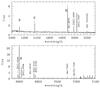 |
Fig. A.1 Total spectrum. The flux is the sum of an extraction centred on 21:21 and summed up within a radius of eight pixels. The upper panel shows the spectrum from the grism HRB, the lower from the grism HRR. The visibility of Hei lines and the absence of the Oii-4636 line already indicate a low temperature and accordingly a high metallicity, which is confirmed by a more detailed line diagnostics. |
All Tables
Diagnostic line ratios (Cols. 3–7) and results from empirical calibrations (Cols. 8–10).
All Figures
|
Fig. 1 HST image and line maps of SH2. All panels have a size of 27″ × 27″ corresponding to 2.33 × 2.33 kpc2. The 5′′ scale bar corresponds to 432 pc. Upper left panel: F555W HST-WPC2 image, matching the line and continuum maps. Upper right panel: continuum map from the HRB grism spectra, using median values. Lower left panel: Hα flux map from the HRR instrument set-up. Lower right panel: map of the [Oiii]-line at 5007 Å using the HRB set-up. In all frames north is towards the top and east is left. |
| In the text | |
|
Fig. 2 Left panel: radial velocity map of the SH2 region. Neither rotation nor velocity gradients are visible. The globular cluster 429 is offset by about −30 km s-1 from the main body of SH2. The object in the north-western region (also visible in Fig. 1) is a background galaxy without emission lines. The velocity is therefore not valid and the redshift is unknown. Right panel: velocity dispersion map of SH2. Except for the south-western region that is also the zone of the brightest Hα-emission, the dispersion is higher than expected from simple stellar-dynamical considerations. An interesting feature is that the spot with the highest dispersion coincides with the highest [Oiii]-flux intensity (see lower right panel of Fig. 1). |
| In the text | |
|
Fig. 3 Approximate locations and approximate sizes of the extraction radii of our characteristic spectra. The image is the median of the HRblue data cube. The unusual X-Y-configuration reflects the axes on the original data cube. |
| In the text | |
|
Fig. 4 Diagnostic graphs for six selected emission line spectra in SH2 (see Table 3 and Sect. 5.2 for explanation). These spectra are compared to Hii region models from Dopita et al. (2013) with the ionisation parameter log q and four oxygen abundances (0.5 × solar, solar, 2 × solar, and 3 × solar) as parameters. The solid lines are lines of constant oxygen abundance and varying log q. In the left panel, the range of log q values is indicated, and is the same for all panels. The models refer to κ = ∞ (corresponding to a Boltzmann electron distribution). The dotted lines in the middle and right panels separate Hii regions from AGN- and LINER-spectra according to Kewley et al. (2001). All spectra except 25:17 are consistent with a uniform abundance value, although [Oiii]/Hβ varies significantly. The middle and the right graph show the degeneracy for high metallicities that is not present in the left graph. A super-solar oxygen abundance is supported by all three diagnostic graphs. |
| In the text | |
|
Fig. A.1 Total spectrum. The flux is the sum of an extraction centred on 21:21 and summed up within a radius of eight pixels. The upper panel shows the spectrum from the grism HRB, the lower from the grism HRR. The visibility of Hei lines and the absence of the Oii-4636 line already indicate a low temperature and accordingly a high metallicity, which is confirmed by a more detailed line diagnostics. |
| In the text | |
Current usage metrics show cumulative count of Article Views (full-text article views including HTML views, PDF and ePub downloads, according to the available data) and Abstracts Views on Vision4Press platform.
Data correspond to usage on the plateform after 2015. The current usage metrics is available 48-96 hours after online publication and is updated daily on week days.
Initial download of the metrics may take a while.