| Issue |
A&A
Volume 601, May 2017
|
|
|---|---|---|
| Article Number | A15 | |
| Number of page(s) | 10 | |
| Section | Planets and planetary systems | |
| DOI | https://doi.org/10.1051/0004-6361/201630017 | |
| Published online | 21 April 2017 | |
Dynamical rearrangement of super-Earths during disk dispersal
I. Outline of the magnetospheric rebound model
1 Anton Pannekoek Institute (API), University of Amsterdam, Science Park 904, 1090 GE Amsterdam, The Netherlands
e-mail: This email address is being protected from spambots. You need JavaScript enabled to view it.
; This email address is being protected from spambots. You need JavaScript enabled to view it.
2 Department of Astronomy and Astrophysics, University of California, Santa Cruz, CA 95064, USA
e-mail: This email address is being protected from spambots. You need JavaScript enabled to view it.
3 Institute for Advanced Studies, Tsinghua University, 100086 Beijing, PR China
4 Kavli Institute for Astronomy & Astrophysics, Peking University, 100871 Beijing, PR China
5 National Astronomical Observatory of China, 100012 Beijing, PR China
Received: 6 November 2016
Accepted: 3 February 2017
Abstract
Context. The Kepler mission has discovered that close-in super-Earth planets are common around solar-type stars. They are often seen together in multiplanetary systems, but their period ratios do not show strong pile-ups near mean motion resonances (MMRs). One scenario is that super-Earths form early, in the presence of a gas-rich disk. These planets interact gravitationally with the disk gas, inducing their orbital migration. However, for this scenario disk migration theory predicts that planets will end up at resonant orbits due to their differential migration speed.
Aims. Motivated by the discrepancy between observation and theory, we seek a mechanism that moves planets out of resonances. We examine the orbital evolution of planet pairs near the magnetospheric cavity during the gas disk dispersal phase. Our study determines the conditions under which planets can escape resonances.
Methods. We extend Type I migration theory by calculating the torque a planet experiences at the interface of the empty magnetospheric cavity and the disk, namely the one-sided torque. We perform two-planet N-body simulations with the new Type I expressions, varying the planet masses, stellar magnetic field strengths, disk accretion rates, and gas disk depletion timescales.
Results. As planets migrate outwards with the expanding magnetospheric cavity, their dynamical configurations can be rearranged. Migration of planets is substantial (minor) in a massive (light) disk. When the outer planet is more massive than the inner planet, the period ratio of two planets increases through outward migration. On the other hand, when the inner planet is more massive, the final period ratio tends to remain similar to the initial one. Larger stellar magnetic field strengths result in planets stopping their migration at longer periods. We apply this model to two systems, Kepler-170 and Kepler-180. By fitting their present dynamical architectures, the disk and stellar B-field parameters at the time of disk dispersal can be retrieved.
Conclusions. We highlight “magnetospheric” rebound as an important ingredient able to reconcile disk migration theory with observations. Even when planets are trapped into MMRs during the early gas-rich stage, subsequent cavity expansion induces substantial changes to their orbits that move them out of resonance.
Key words: methods: numerical / planet-disk interactions / stars: magnetic field / planets and satellites: formation
© ESO, 2017
1. Introduction
The Kepler and K2 transit missions have together discovered over 3300 exoplanets and 500 multi-planet systems. These data constitute a large sample to statistically analyze the properties of exoplanets. The majority of planets discovered by Kepler are close-in super-Earths, namely planets with radii Rp< 4 R⊕ or mass Mp ≲ 10 M⊕, and periods P< 100 days. Super-Earths are very common: nearly half of solar-type stars harbour one or more super-Earth (Petigura et al. 2013). This occurrence rate appears to be independent (or at most weakly dependent) on stellar type and metallicity (Howard et al. 2012; Fressin et al. 2013; Mayor et al. 2011; Bonfils et al. 2013; Mulders et al. 2015). The mass of several tens of super-Earths are known from follow-up radial-velocity or transit-timing variation (Lithwick et al. 2012; Marcy et al. 2014), and combined with the radii, allow us to obtain the bulk densities. For many of them, bulk densities are too low to be consistent with a pure rocky composition: a hydrogen-helium atmosphere is required. In order to acquire such a substantial gaseous atmosphere, super-Earths are inferred to have formed in early the gas-rich disk phase, before the depletion of the disk gas (Lopez & Fortney 2014; Rogers 2015).
Super-Earths are frequently found in multiple, compact systems with relatively low eccentricities and inclinations (Fang & Margot 2012; Fabrycky et al. 2014; Shabram et al. 2016; Xie et al. 2016). Their orbits neither exhibit strong pile-ups at mean motion resonances (MMRs) nor are their period ratios uniformly distributed (Fig. 6 of Winn & Fabrycky 2015). In particular, the period-ratio distribution shows an asymmetry around major resonances with a deficit abundance just interior to, and an excess slightly exterior to, the 2:1 and 3:2 MMRs. Also, a significant fraction of planets are found with period ratios much larger than 2.
Planets embedded in disks gravitationally interact with, and transfer angular momentum to the disk gas, resulting in their orbital migration. For low-mass planets, this mechanism is known as Type I migration (Lin & Papaloizou 1979; Goldreich & Tremaine 1979; Kley & Nelson 2012; Baruteau et al. 2014). Theoretically, resonance capture is a natural outcome of planet migration (Lee & Peale 2002; Papaloizou & Szuszkiewicz 2005; Pierens & Nelson 2008). The existence of some resonant systems, such as Kepler-223 (Mills et al. 2016), proves the fidelity of disk migration theory. However, as mentioned above, statistically, the majority of super-Earths are not in MMRs. This discrepancy is a key mismatch between observation and theory.
Different scenarios have been proposed to explain the observed deviation from exact resonance. These include tidal damping of planets (Lithwick & Wu 2012; Delisle et al. 2012; Batygin & Morbidelli 2013; Lee et al. 2013; Xie 2014; Delisle et al. 2014), planet mass growth (Petrovich et al. 2013), interaction with planetesimals (Chatterjee & Ford 2015), stochastic torques in turbulent disks (Rein 2012; Batygin & Adams 2017), planet-wake interaction (Baruteau & Papaloizou 2013), and resonant overstability (Goldreich & Schlichting 2014; Delisle et al. 2015). But these models are mostly limited to small departures – at a few percent level – from resonance. Other scenarios (Ogihara & Ida 2009; Cossou et al. 2014; Ogihara et al. 2015) propose that giant impacts scatter planets away from original resonances after the dispersal of the disk gas. However, these models may not be able to explain the above asymmetry around major resonances. The onset of this orbital instability also requires a sufficient amount of embryos (typically N ≫ 2) in a compact configuration at early stage. Nevertheless, neither of above scenarios have considered the influence of the stellar magnetic field.
T Tauri stars are magnetically active with observed field strengths of kilogauss-level at their surfaces (Johns-Krull 2007). For comparison, the current B-field of the Sun is only 0.3 G. The stellar magnetic field truncates the disk at the magnetospheric cavity radius (Koenigl 1991). This radius is determined by equating the stellar magnetic torque with the viscous torque of the disk. Adopting parameters for a typical T Tauri star, the magnetospheric cavity radius is around 0.1 AU. The size of this cavity increases with time as the viscous torque diminishes during the disk dispersal. In this paper we explore how the expanding cavity affects the dynamical evolution of super-Earth planets.
We propose a new model, magnetospheric rebound, which considers the migration of planets near the magnetospheric cavity. Generally, during the disk dispersal, planets that are trapped in MMRs can migrate outwards together with the expanding magnetospheric cavity. However, when the cavity expansion rate is high or when the disk is no longer massive, the planet will be left behind. Therefore, each planet subsequently drops into the cavity at the time determined by their mass, the disk mass and the gas depletion timescale. As a consequence, planets can substantially alter their dynamical configuration with the cavity expansion during gas disk dispersal, in some cases resulting in the break-up of the MMR.
In this paper, we will test this magnetospheric rebound model by using N-body simulations. The key parameters, apart from the planet masses, are the initial disk accretion rate, the gas disk depletion timescale, and the stellar magnetic field strength. In Sect. 2, we start by presenting the disk model and review the Type I migration torque formulas. In Sect. 3, we carry out numerical simulations and demonstrate the illustrated runs. Two observed Kepler systems are modelled in our parameter study in Sect. 4. Finally, we discuss the results and draw conclusions in Sect. 5.
2. Method
In this section, we give a description about the adopted disk model (Sect. 2.1), which includes the magnetospheric cavity that truncates the disk at a radius rc (Sect. 2.2), and we provide expressions for the Type I torques that act on the planets (Sect. 2.3). Section 2.4 outlines under which conditions the model is applicable.
2.1. Disk model
We considered a disk model with a constant aspect ratio  (1)where H is the disk scale height and r is the disk radius. The corresponding gas disk temperature was:
  (2)where G is gravitational constant, Rg is gas constant, M⋆ is the stellar mass, and μ is the molecular weight in the protoplanetary disk.
The gas surface density (Σ) was derived from the gas accretion rate Ṁg by the steady-state assumption for viscous disks (Ṁg = 3πΣν). We used the Shakura & Sunyaev (1973)α prescription for viscosity, ν = ανH2Ω, where Ω is the Keplerian angular frequency. We focused on the migration of close-in super-Earths for which the disk region is primarily Magnetorotational instability (MRI) turbulent and therefore αν = 10-2 was adopted in this paper. The gas surface density was then given by  (3)Our study concerns the late phase of disk evolution when the gas disk dispersal takes place. We assumed the disk gas accretion rate follows:
 ![Mathematical equation: \begin{equation} {\dot M}_{\rm g} = {\dot M}_{\rm g0} \exp\left[- t/\taud\right], \label{eq:taudep} \end{equation}](/articles/aa/full_html/2017/05/aa30017-16/aa30017-16-eq31.png) (4)where τd is the characteristic disk depletion timescale in late stage. We note that τd is shorter than the typical lifetime of the disk (~ 2–3 Myr, Mamajek 2009) by at least one order of magnitude (Williams & Cieza 2011).
(4)where τd is the characteristic disk depletion timescale in late stage. We note that τd is shorter than the typical lifetime of the disk (~ 2–3 Myr, Mamajek 2009) by at least one order of magnitude (Williams & Cieza 2011).
2.2. Inner magnetospheric cavity
Young T Tauri stars are observed with strong magnetic fields of ~0.2 to 6 kG (Johns-Krull 2007; Yang & Johns-Krull 2011; Johns-Krull et al. 2013). The stellar magnetic field lines are strongly coupled to the disk gas close to the central star. The Lorentz torque is generated by the stellar-disk magnetic interaction whereas the viscous torque is induced by the disk gas. The inner disk is truncated at the radius where the Lorentz torque is greater than the viscous torque (Ghosh & Lamb 1979; Koenigl 1991; Armitage 2010). The gas flow near the cavity edge is accreted onto the stellar surface along field lines, which is known as magnetospheric accretion. We assumed that the gas inside the cavity (r<rc) is removed very quickly and therefore that the inner edge of the disk is sharply cut off (Fig. 1). The magnetic torque per unit area is B2r/ 2π and the viscous torque is  . Assuming that the central star has a dipole magnetic field (
 ) aligned with the stellar rotation axis, the size of this magnetospheric cavity is (Frank et al. 1992; Armitage 2010):
  (5)where G is the gravitational constant, B⋆ is the magnetic field strength at the stellar surface, R⋆ is the stellar radius and ΩK is the angular velocity at distance r. Adopted from the fiducial value of T Tauri stars, namely M⋆ = 1 M⊙, R⋆ = 2 R⊙, Eq. (5) evaluates as
  (6)From Eq. (6), it is clear that the cavity expands with decreasing Ṁg, which is a consequence of the diminishing importance of the viscous torque.
Equation (6) is based on two assumptions. Firstly that the stellar magnetic field is dipole, and secondly that the magnetic axis is aligned with the stellar rotation axis. In reality, the field can contain higher-order contributions, for example quadrupole term  that could dominate at stellar distances r ~ R⋆. However, at the larger distances that are important for this study the dipole contribution takes over. Also, both theoretical analyses (Lipunov & Shakura 1980; Lai et al. 2011) and MHD simulations of magnetospheric accretion (Romanova et al. 2003, 2004) indicate that when the magnetic field axis is misaligned with the rotation axis of the disk, the inner disk is likely to be warped. In that case the gas density distribution is not axisymmetric as in Eq. (3). Nonetheless, many of the features that we use in the axisymmetric case would still be present: there would still be a magnetospheric cavity that expands during the disk dispersal, and there would still be a one-sided planet-disk interaction (as discussed in Sect. 2.3). However, to model this additional complexity is beyond the scope of this paper.
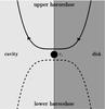 |
Fig. 1 Sketch of the gas’ motion near the cavity edge. The gas only completes the upper horseshoe U-turn before it is accreted to the central star by magneto-stellar forces, which we assume to remove the gas very quickly. There is no gas left to execute the lower horseshoe. |
With decreasing Ṁg, the truncation radius rc becomes larger than the corotation radius rco, which is the radius where the disk’s Keplerian frequency equals the spin frequency of the star. In principle, when rc>rco accretion is quenched and the angular momentum is transferred from the stellar spin to the disk. However, this process also leads to a stellar spin-down and the expansion of the corotation radius. Provided the disk depletion time is sufficiently long or that the spin synchronization proceeds rapidly, rc and the corotation radius expand in tandem and accretion onto the host star is maintained. Observationally, Kepler target stars have modest spin periods up to a few months (McQuillan et al. 2014), generally longer than the orbital periods of the inner-most super-Earths. Therefore, these systems could have experienced an expansion of the corotation radius at the time of disk dispersal. For simplicity, in this work we assume that the disk truncation radius is given by Eq. (6) and that the disk always accretes onto the star.
2.3. Type I torques acting on the planet
Having specified a model for the gas structure, we now discuss the backreaction of the disk on the planet. The key point in our discussion is the distinction between two-sided torques and one-sided torques. A sketch illustrating the difference between one-sided and two-sided torques is shown in Fig. 2. Two-sided torques apply when the planet is far away from the disk cavity (Fig. 2a). In that case it experiences the inner and outer Lindblad torques from both sides. Usually, the net (differential) value is negative, causing inward migration (Ward 1997). The corotation torque is determined by the gradient of disk surface density and temperature across the horseshoe region of the planet. It is described in Sect. 2.3.1. One-sided torques are applicable when the planet is at the cavity edge (Fig. 2b). In that case it experiences a negative, one-sided Lindblad torque and a positive one-sided corotation torque. One-sided torques are generally much larger than two-sided torques, because the near-cancellation effect – a feature of the two-sided torques – is absent. The descriptions of one-sided Lindblad torque and one-sided corotation torque will be given in Sects. 2.3.2 and 2.3.3. In Sect. 2.3.4 a general Type I torque that combines these two regimes is presented.
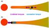 |
Fig. 2 Sketch illustrating the difference between two-sided and one-sided torques. a) When the planet is far away from the disk cavity, it experiences two-sided torques from the disk. b) When the planet is at the cavity edge, only one-sided torques operate. The purple and blue arrows denote the Lindblad and corotation torques, respectively. |
2.3.1. Two-sided torques
When the planet is far from the disk edge and embedded in a continuous disk, the interior disk exerts a positive torque and pushes the planet outwards, whereas the exterior disk pushes it inwards. To first order, these contributions cancel. The “standard” two-side Lindblad torque (ΓL,2s) is therefore a differential torque, the sign of which is determined by the gradient of the disk structure (Goldreich & Tremaine 1980; Tanaka et al. 2002). In addition, the planet interacts with the gas within the co-orbital horseshoe region (the two-sided corotation torque).
Considering these two torque components, we adopted the total two-sided torque from Eq. (49) of (Paardekooper et al. 2010, local isothermal approximation), ![Mathematical equation: \begin{eqnarray} \begin{split} & \frac{\Gamma_\mathrm{2s}} {m_{\rm p} (r_{\rm p} \Omega_{\rm p})^2} = \frac{\Gamma_\mathrm{L,2s} + \Gamma_\mathrm{c,2s} } {m_{\rm p} (r_{\rm p} \Omega_{\rm p})^2}=\\ & \qquad \left[-(2.5 + 0.5\beta +0.1s) + 1.4\beta + 1.1\left(\frac{3}{2} +s\right) \right] q_{\rm d} \frac{q_{\rm p}}{h^2}, \label{eq:2s} \end{split} \end{eqnarray}](/articles/aa/full_html/2017/05/aa30017-16/aa30017-16-eq55.png) (7)where β is the gradient of temperature, s is the gradient of gas surface density,
(7)where β is the gradient of temperature, s is the gradient of gas surface density,  and qp ≡ mp/M⋆ are dimensionless measures of the local disk mass and planet mass, respectively. The notation Xp indicates the quantity X evaluated at the planet location r = rp. The first term on right hand side of Eq. (7) describes the two-sided Lindbald torque (ΓL,2s) and the other two terms represent the two-sided corotation torque (Γc,2s).
2.3.2. One-sided Lindblad torque
However, when a planet approaches the inner edge of the disk the torques from the exterior disk start to dominate over those from the interior disk. In the limit of a vanishing interior disk, the planet only experiences negative Lindblad torques from the exterior disk. No longer is the torque a result from a near-cancellation of two large contributions. Instead, the torque has become a first-order effect. We denoted this torque as ΓL,1s.
The one-sided Lindblad torque can be calculated from the impulse approximation (Lin & Papaloizou 1979, 1993):  (8)where b = r−rp is the separation between each annular gas parcel and the planet, and bmin = 2H/ 3 is a cutoff boundary adopted for the torque density (Ward 1997; Artymowicz 1993). We then obtained for the one-sided Lindblad torque:
  (9)where the prefactor CL = −0.65.
2.3.3. One-sided corotation torque
We next calculated the corotation torque for when the planet is at the cavity edge. In the context of a one-sided co-rotation torque, only the upper horseshoe is present (where material is transported from orbits exterior to the planet to orbits interior to the planet, Fig. 1). The lower horseshoe motion is absent by virtue of the assumption that any gas interior to the planet is quickly removed along magnetic field lines and accreted to the central star. Therefore, the planet exchanges angular momentum only through the upper horseshoe, which provides a strong positive corotation torque. We denoted this torque the one-sided corotation torque Γc,1s. It can be calculated from angular momentum conservation principles, meaning that the angular momentum lost due to material being pushed to a lower Keplerian orbit is gained by the planet. Following Paardekooper & Papaloizou (2009):  (10)where j = ΩK(r)r2 is the specific angular momentum corresponding to r. We adopted xhs = 1.7(qp/h)0.5rp (Paardekooper & Papaloizou 2009; Ormel 2013) for the half-width of the horseshoe region and obtained
  (11)where Chs = 2.46.
Based on the assumption that gas is removed quickly at the edge of the disk, the surface density has a infinitely sharp transition at rc. Under this assumption, the planet obtains its maximum positive one-sided corotation torque and it maximizes the rebound (outward migration). For simplicity, we only consider this situation. Instead, if gas removal is not an efficient process, there could be a more gradual transition in which Σ is (locally) a power-law. In that case, the Lindblad and corotation torques at rc are determined by the two-sided torques expression and the rebound is reduced but does not diminished. Nevertheless, three-dimensional MHD simulations of magnetospheric accretion (Romanova et al. 2002) reveal a strong cut-off of the gas density near the disk edge that supports our approximation.
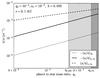 |
Fig. 3 Planet migration rate (ȧ/a) for different torques as a function of dimensionless planet mass qp = Mp/M⋆ ar r = 0.1 AU. The dotted, solid, and dashed lines correspond to the migration rate estimated from Eq. (12) when Γ = Γ2s (two-sided torque), ΓL,1s (one-sided Lindblad torque) and Γc,1s (one-sided corotation torque), respectively. The dark grey zone refers to the non-linear regime, and the light grey zone indicates the gap-opening regime. qp,gap and qp,lin are the critical masses for these two regimes (Sect. 2.4). The adopted disk parameters are qd = 10-4, αν = 10-2 and h = 0.025. |
The migration rate corresponding to a torque (Γ) is  (12)In Fig. 3, the migration rate (ȧ/a) is plotted for the two-sided torque Γ2s, the one-sided corotation torque Γc,1s, and the one-sided Lindblad torque ΓL,1s as a function of qp at r = 0.1 AU. The dark grey zone indicates the non-linear regime and the light grey zone indicates the gap-opening regime (see the discussion in Sect. 2.4). Two-sided torques are second-order torques, the sign of which depend on the gradient of the disk profile in the vicinity of the planet (Eq. (7)). However, one-sided torques are independent of s and β (Eq. (11) and Eq. (9)). Indeed, one-sided torques are larger than two-sided torques (approximately by a factor h-1). Between the one-sided torques, the positive corotation torque is larger than the negative Lindblad torque when qp is small. As previously mentioned, the one-sided torques operate for the disk region near the cavity whereas the two-sided torques operate for the disk region away from the cavity. Therefore, small planets are able to migrate outwards from the disk edge until the point where the two-sided torques dominate. This also means that small planets can migrate outwards when the cavity gradually expands.
However, when the planet is large enough to enter the gap-opening regime, the corotation torque diminishes due to the depletion of gas in the horseshoe region. Then, the (negative) one-sided Lindblad torque would be in magnitude larger than the (positive) one-sided corotation torque. In that case, the planet directly migrates into the cavity and is left behind as the disk cavity (rc) expands.
Since the eccentricities of planets could be excited by planet-planet interaction, we also considered the saturation of the corotation torque (both one-sided and two-sided, Bitsch & Kley 2010): ![Mathematical equation: \begin{equation} \Gamma_{\rm c}(e) = \Gamma_{\rm c} (0) \exp\left[-e/e_{\rm f}\right], \label{eq:sat} \end{equation}](/articles/aa/full_html/2017/05/aa30017-16/aa30017-16-eq93.png) (13)where e is the eccentricity of the planet, Γc(0) is the corotation torque for zero eccentricity, and ef = h/ 2 + 0.01 (Fendyke & Nelson 2014).
(13)where e is the eccentricity of the planet, Γc(0) is the corotation torque for zero eccentricity, and ef = h/ 2 + 0.01 (Fendyke & Nelson 2014).
2.3.4. Combined Type I torque
A more general case applies when a planet approaches the disk edge that falls in between the one-sided and embedded (two-sided) regimes discussed above. In that case, the torque expression is approximated by interpolating the one-sided and two-sided torques:  (14)where the coefficient f = exp[−(r−rc) /xhs] is a measure of the proximity of a planet to the disk edge, in which f = 1 at the edge and f = 0 far away from the edge. The form of the expression ensures that the total torque is dominated by the one-sided torque when the planet is located within a half-horseshoe width from the disk edge (rp ≤ rc + xhs).
2.4. Model applicability
Our expressions for the Type-I torques are valid in the linear regime where the planet’s perturbation is small. This requires the planet’s Hill radius to be smaller than the disk scale height (RH ≡ (mp/ 3M⋆)1/3<H, Lin & Papaloizou 1993). This condition can be expressed as:  (15)The non-gap-opening criterion also requires that the planet torque (Γp) is smaller than the viscous torque (Γν = 3πΣνr2Ω). Otherwise the disk does not supply enough material (angular momentum) to fuel the planet. This condition is especially relevant to planets at the disk edge rc where the planet torque is dominated by the one-sided corotation torque, Γp = Γc,1s (Eq. (11)). The no-gap opening condition reads
  (16)or
  (17)For typical super-Earth planets (Mp ≲ 10 M⊕) around solar type stars, the above two conditions require h ≳ 0.025 near the edge of the disk. In addition, the no-gap opening condition requires a large αν parameter. This explains our default values for h and αν. The Γc,1s is the torque that provides planet outward migration near the cavity edge. For very low h and αν disks, gaps can be opened by super-Earth planets and Γc is reduced because the gas is severely depleted in their horseshoe regions. As a consequence, we do not expect the magnetospheric rebound mechanism to operate in systems with low h and αν.
But how realistic are our adopted values of h and αν? Typically, MHD simulations modelling the MRI (Balbus & Hawley 1998) indicate α ≃ 10-2 (Davis et al. 2010; Suzuki et al. 2010), provided that the disk is sufficiently ionized. Generally, this holds true for the very inner disk (≳103 K) where thermal ionization of alkali elements produces the required amount of electrons (Armitage 2011). However, as the cavity radius (rc) expands, the temperature drops and ionization becomes dependent on non-thermal processes (e.g., stellar X-ray irradiation). Although initially the high densities should prevent X-rays from penetrating the disk midplane, the expansion of the cavity radius also quickly decreases Σ since  (Eqs. (3) and (5)). In addition, we note that because we study the inner disk (a ≲ 0.3 AU) at late times, small dust grains have coagulated into large bodies. In such a dust-free medium, the liberated electrons always end up in the gas, increasing the electron fraction and promoting the MRI.
The disk’s aspect ratio is determined by a thermal balance: an increased midplane temperature increases h (Eq. (2)). A high midplane temperature can result from viscous dissipation (a high Ṁ) in combination with a large vertical optical depth. But as the disk evolves at late stage, a higher T can also arise when the (visible) optical depth is low and stellar photons penetrate the disk deeper. For example, in the optically-thin limit, the equilibrium temperature at 0.1 AU for a solar-mass star would be 1200 K, corresponding to a scale height of 0.022. In addition, magnetic accretion generates additional heat near the cavity edge (Hartmann et al. 1998), further increasing the aspect ratio h.
Based on these considerations, we believe that the adopted values of h = 0.025 and α = 10-2 are reasonable. It should be noted that we assumed a constant aspect ratio in this paper, which is independent of r. We also investigated another aspect ratio profile, h = 0.05r1/5, and found that the results presented in the following sections are only weakly affected. Overall, our results should be applicable to super-Earth planets as long as the inner disk is hot enough.
In addition, the magnetospheric accretion process requires efficient coupling between the field lines and the disk gas. This condition implies that the magnetic diffusivity η is sufficiently small, η ≲ Hcs (Wardle 2007). The criterion for the onset of MRI is that the magnetic Reynolds number is larger than one, Re (Armitage 2010), where cs and vA are the sound speed and Alfvén speed. This suggests
  . Therefore, the disk always satisfies the coupling condition once the MRI is operational. The model is applicable because we study super-Earth systems with typical orbital periods of a few weeks around their host stars.
Adopted parameters.
Ogihara et al. (2010) also calculate a torque near the disk edge, which they term the “edge torque”. This torque operates for eccentric planets at the disk edge, which experience asymmetric eccentricity damping from the disk gas. The magnitude of the edge torque increases with the eccentricity of the planet. However, when calculating the total torque in their Eq. (17), Ogihara et al. (2010) still use the two-sided Type I torque expression. As we demonstrate in this paper, when the planet is near the disk edge, one-sided torques will dominate over two-sided torques. Also, we find that the eccentricities of the planets are modest, a few times 10-2, in our simulations. For these low eccentricities, the one-sided torque (Eq. (11)) is much larger than the edge torque (Eq. (15) of Ogihara et al. 2010). We therefore neglect the edge torque in this paper.
3. Results
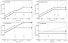 |
Fig. 4 Migration of a planet pair in the gaseous disk. Black lines trace the time evolution of the semi-major axes of the planets and the blue dashed line represents the inner magnetospheric radius rc. The four panels show simulations with a) default parameters; b) massive inner planet; c) strong stellar magnetic field and d) a light disk. Parameters are listed in Table 1. Vertical lines represent the time when the inner (t1) and the outer planet (t2) enter the cavity. We would like to note that the scale of the x-axis of panel d) is different from the others. |
We carried out numerical experiments using Hermite N-body code (Aarseth 2003). In this code, the planet-planet interaction is calculated with the Hermite scheme, and the planet-disk interaction is included by adding additional torque recipes (details are available in Liu et al. 2015). However, Liu et al. (2015) only consider the two-sided torques (Paardekooper et al. 2011). In this work, we add the new torque formulas demonstrated in the previous section that are a combination of both one-sided and two-sided torques. Another difference is that this work considers the locally isothermal limit, which is applicable to the late disk dispersal phase when the disk opacity is substantially reduced.
The goal of our simulations is to investigate the evolution of the period ratio of the planet pair during the dispersal of the gas disk. In this paper, only two-planet systems are considered. The simulations were performed until the disk gas was entirely depleted. Because the long-term secular evolution of a two-planet system does not change their orbits once the planets are in the Hill stable regime, we considered the orbits of planets at the end of simulations to be their present-day orbits. A set of simulations (referred to as run 1 to 4) with different planet masses (Min and Mout), disk properties (Ṁ, τd), and stellar magnetic field strengths (B⋆) were performed. We set M⋆ = 1 M⊙ throughout this section. The adopted parameters are given in Table 1 and the results are illustrated in Fig. 4.
3.1. Planet pair with more massive outer planet
The result from the default run is presented in Fig. 4a. The parameters were set as Ṁg0 = 10-8M⊙ yr-1, τd = 105 yr and B⋆ = 1 kG. Initially, the magnetospheric cavity radius (rc) is at 0.052 AU and two embryos are located at 0.052 AU and 0.076 AU. Their orbits are hence initialized between the 3:2 and 2:1 MMRs. The inner and outer planet masses are 3 M⊕ and 6 M⊕.
Because of convergent migration, the planets soon get trapped in the 3:2 MMR and migrate inward to the magnetospheric cavity within a few thousand years. When the inner planet gets close to the cavity edge (rin ≃ rc), one-sided torques become dominant. For this combination of disk and planet parameters, the outward (positive) one-sided horseshoe torque is larger in magnitude than the inward (negative) one-sided Lindblad torque (Γ1s,hs + Γ1s,L > 0). Since the outer planet is far away from the disk edge in terms of horseshoe units, (rout−rc) /xhs ≫ 1, its torque is still in the two-sided regime and negative. However, the sum of the torques on both planets is dominated by the one-sided torque from the inner planet and evaluates to a net positive value.
Whether or not the planet pair migrates outwards is determined by two timescales: the planet migration timescale τm (= (ȧ/a)-1, Eq. (12)) and the cavity expansion timescale τc (that approximately equals 3.5τd, Eq. (6)). If the cavity expands at a speed much larger than the migration of the planet, it overtakes the planet. The planet then falls into the cavity and ceases migrating. Otherwise, when τm < τc, it keeps migrating with the expansion of the cavity. Because τm <τc initially, the total disk torques drive the outward migration of both planets. However, as Ṁg(t) decreases with time, the disk gas mass diminishes, which increases the migration time τm. Therefore, at some point τm(t) becomes longer than τc, indicating that the disk can no longer accommodate the migration of both planets. The inner planet therefore drops into the inner cavity radius rc (blue dashed line in Fig. 4). We find that this occurs at t1 = 3.0 × 10⁵ yr.
After t = t1, the planet pair initially moves inwards, because the net torque is now due to the outer planet and the planets are still in resonance. However, the planet pair decouples from MMR when the expanding cavity approaches the outer planet (rout ≃ rc). After that, only the outer planet is able to migrate outwards with the cavity expansion. This is because divergent migration leads to resonance crossing rather than resonance trapping (Henrard & Lemaitre 1983; Murray & Dermott 1999). Eventually, the outer planet ceases migrating at around 5.6 × 10⁵ yr when its migration timescale becomes longer than the cavity expansion timescale. We denote this time t2. After t = t2 both planets are within the magnetospheric cavity. After the gas is entirely depleted, the planets end up at 0.116 AU and 0.254 AU. Their final outer-to-inner period ratio (Pout/Pin) is 3.24, much larger than the original 3:2 resonance.
3.2. Planet pairs with more massive inner planet
We show the result of run 2 in Fig. 4b. It had identical model parameters as the default run, except that the mass order of the planets was changed: Min = 6 M⊕ and Mout = 3 M⊕.
Similar to run 1, initially both planets migrate to the cavity edge in the 3:2 MMR. Likewise, the migration timescale for the pair (τm) is shorter than τc and therefore both planets migrate outwards with the expansion of the cavity. After a while, the inner planet ceases migrating when the expansion rate of the cavity starts to exceed the migration rate of the two resonant planets. This occurs at t1 = 4.6 × 10⁵ yr. It is later than the time in run 1 (3.0 × 10⁵ yr). When the cavity radius rc approaches the outer planet at t2 = 5.7 × 10⁵ yr, it directly falls in without substantial outward migration as run 1. Consequently, their final period ratio Pout/Pin = 1.57 is still close to the 3:2 MMR.
Why are the final period ratios between run 1 and run 2 so different when only their mass ratio has changed? The small outer-to-inner mass ratio in run 2 has two significant effects. First, the torques’ contribution from the inner massive planet becomes even more dominant. It means that the inner planet falls into the cavity at a later time (t1 in run 2 is larger). Therefore, both planets migrate farther out when the inner planet is more massive. Second, rc only approaches the outer planet at a later time when the disk mass is relatively low. A lower disk mass and a less massive outer planet leads to subsequently slower outward migration. As a consequence, when the cavity approaches the outer planet in run 2, its migration timescale is already longer than the cavity expansion timescale. Hence, the outer planet drops into the cavity and their orbits still remain close to the 3:2 MMR.
3.3. Strong stellar magnetic field
We performed run 3 with the same planet masses and disk parameters as the default run, but with a stronger stellar magnetic field of B⋆ = 5 kG. The result is presented in Fig. 4c. For this strong B-field, rc = 0.13 AU at the beginning. This is because the magnetospheric cavity is determined by the dominant stellar magnetic torque. As shown in Eq. (6), larger B⋆ results in a stronger magnetic torque that truncates the inner disk farther out. The embryos’ migration behaviours are similar to the default run. They enter into the cavity at the same time (t1 and t2) and stop at the same period ratio as run 1. The reason is that the time when the planets enter the cavity depends on the comparison between planet migration timescale and the cavity expansion timescale, both of which are independent of the B⋆. However, the stronger B-field carries the planets farther away and the final orbits of the two planets end up at 0.292 AU and 0.637 AU.
3.4. Light disk
Finally, we performed a run with the same planet masses as run 1 (Min = 3 M⊕,Mout = 6 M⊕) but different disk parameters (Ṁg0 = 5 × 10⁻¹⁰M⊙ yr-1, τd = 104 yr). Here the initial disk accretion rare (Ṁg0) decreases by a factor of 20 and the disk depletion time (τd) reduces by a factor of 10. Low Ṁg0 indicates that the initial disk mass is low and short τd means that the gas is depleted rapidly. The combination of these two parameters implies a light disk (small Σ or qd) during the evolution timespan simulated here. In contrast to the massive disk in the default run, the light disk can not provide sufficient angular momentum exchange to the planets. Therefore, the planet migration timescale τm is always longer than the cavity expansion timescale τc in this case. Both planets result in only minimal change of their orbits. The final period ratio of the planet pair is 1.72, very close to its initial value (Fig. 4d).
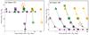 |
Fig. 5 Scatter plot of the inner period of the planet and the period ratio of the outer-to-inner planet. The left and right panel present the results of Kepler 170 and Kepler 180, repsectively. The red star represents the observed data and other symbols give the results of numerical simulations. Symbols correspond to stellar magnetic field strengths B⋆ where B⋆ equals 0.3 kG (triangle), 1 kG (square) and 3 kG (circle). Colour corresponds to the disk dispersal timescale (τd) where purple, green, and orange mean 103, 104 and 105 yr, respectively. The sizes of the symbols represent the disk accretion rate at the onset of disk dispersal (Ṁg0), ranging from 10-9 (small), 3 × 10⁻⁹, 10-8, 3 × 10⁻⁸ to 10-7M⊙ yr-1 (large). |
4. Modelling Kepler systems
The goal of this section is to compare the observed super-Earth systems with our proposed magnetospheric rebound model. To investigate under which conditions these systems preferentially form, we conducted a parameter study, varying Ṁg, τd and B⋆.
4.1. Set-up for the parameters survey
For our pilot study, we considered two super-Earths systems, Kepler 170 and Kepler 180. Kepler 170 contains two super-Earth planets near the 2:1 MMR, whereas the period ratio of the planets in Kepler 180 is 3.03. Theoretically, planet migration theory dictates that planets formed in gas-rich disks are likely to end up in MMRs. However, the Kepler mission has shown that many super-Earths are at period ratios near but not exactly at MMRs (e.g., 2.2:1; Steffen & Hwang 2015), or that their period ratios are far from any MMRs. Motivated by the representative period ratios of these two systems, we selected them as typical cases and explored why the planets ended up so different.
The planet masses, their periods, and the stellar masses are listed in Table 2. The observed systems were selected from the NASA Exoplanet Archive1 and their planet masses were obtained from Wolfgang et al. (2016)’s mass-radius relationship (their Eq. (1)):  (18)All planets were initialized in coplanar and circular orbits. The inner planets were located at the edge of the inner cavity, and the outer planets started beyond their 2:1 MMR.
Propertes of observed super-Earth system.
The initial gas accretion (Ṁg) rate was sampled as five values in the range of 10-9 to 10-7M⊙ yr-1. The disk dispersal time (τd) was given by three values, 103, 104, and 105 yr. The magnetic field strength (B⋆) was selected from three values, 0.3, 1, and 3 kG. We ran 45 simulations for each system with each simulation referring to one specific combination of the Ṁg0, τd and B⋆ values. The outcomes (Pout/Pin and Pin) are shown in Fig. 5. The left and right panel show the results of Kepler 170 Kepler 180, respectively. The colour, size and shape of the data points refer to τd, B⋆ and Ṁg0, respectively. The red star marks the location of the observed systems in this Pout/Pin−Pin diagram.
4.2. Kepler 170
Kepler 170 is a 0.97 M⊙ star, containing two super-Earth planets, Kepler 170b and Kepler 170c. Based on the radius from the transit and mass-radius relation from Eq. (18), the masses of the planets are 10.59 M⊕ and 9.42 M⊕, respectively. Their periods are 7.93 and 16.67 days, with a period ratio of 2.10.
For this system, the simulated data results in a large spread in the period of the inner planet (x-axis of Fig. 5a), such that Pin ranges from 1.2 to 68 days. With tuning of the parameters, we can easily obtain a perfect match to the inner planet period. Although the simulated period ratios all lie below the observed value, five of them show only minor deviation (~1.3%). We would like to note that all five yellow triangles with different size are stacked at the same period ratio close to 2.07. One may wonder why the simulations cannot reproduce period ratios larger than the observed period ratio. The reason is the empirical mass-radius relationship used here (Eq. (18)). Because of the uncertainty in M(R), the true mass likely deviates from the estimated value. However, a slightly higher outer-to-inner mass ratio will result in a period ratio that matches the observed value which is still consistent with the observational constraints.
In Fig. 5a, we see that for the same initial disk accretion rate and gas depletion timescale, the inner planet period is longer when the stellar B-field is stronger. This can be understood from our previous discussion related to Figs. 4a and c, namely that larger stellar magnetic field strength results in planets stopping their migration at longer periods because the disk cavity radius rc is farther out.
We also see that for the same gas depletion timescale and stellar B-field but for increasing Ṁg0, the period ratio increases from 2 to approximately 2.07. Because planets get trapped into the 2:1 MMR first, they migrate outwards and leave resonance through the cavity expansion. A high  results in substantial outward migration and hence increases their period ratio. An exception is those runs with the strongest stellar B-field. Their final period ratios decrease from 2 to approximately 1.8 with increasing Ṁg0. The reason is that these planets get trapped in 3:2 instead of 2:1 before the magnetospheric rebound operates. Because resonance trapping is related to the migration rate, only planets with fast migration rates (large local disk mass
  , Eq. (12)) are able to bypass the resonance barrier (Ogihara & Kobayashi 2013; Liu et al. 2015, 2016). Both a higher disk accretion rate (larger Σ0) and a larger stellar B-field (larger rp) contribute towards increasing the local disk mass. Therefore, only systems with Ṁg0 and large B⋆ are able to bypass the 2:1 MMR and get trapped into the 3:2 MMR. Finally, magnetospheric rebound pushes the resonant planets outwards and increases the period ratio from the 3:2 MMR to a value between 1.5 to 2 during the disk dispersal phase.
The interpretation of this particular system is applicable to systems that contain nearly equal-mass super-Earths, have close to ten days inner-planet period, and a period ratio slightly in excess of two. These systems follow a similar formation history, and their B⋆, τd, and Ṁg0 can be modelled with the same approach shown here.
4.3. Kepler 180
Kepler 180 is a 1.05 M⊙ star and harbours two super-Earths, Kepler 180b and Kepler 180c. The masses of the planets are 3.90 M⊕ and 9.27 M⊕, and their periods are 13.82 and 41.89 days, respectively. Their outer-to-inner mass ratio is 2.38 and their period ratio is 3.03. The results related to Kepler 180 are presented in Fig. 5b.
One obvious difference between Figs. 5a and b is that the period ratios of simulated planets in Fig. 5b (≳2) can be much larger than those of Fig. 5a (approximately 1.7 to 2.1). Although the planets get quickly trapped in MMRs, they move away from resonance during the magnetospheric cavity expansion. We can understand this behaviour from the simulations conducted in Figs. 4a and b (run 1 and 2). There, the only difference is the mass order of the planets. When the outer-to-inner planet mass ratio is large, the outer planet can continue to migrate extensively after leaving resonance, resulting in a large period ratio. In Kepler 180 the outer planet is more massive than the inner planet, whereas in Kepler 170 the planets are of nearly equal-mass. Consequently, the period ratios in Fig. 5b are larger than those in Fig. 5a.
From Fig. 5b we see that the observed planet periods and their ratio (red star) lie inside the range spanned up by the simulations. Therefore, this system is well-fitted by the magnetospheric rebound mechanism and we are able to constrain key disk and stellar magnetic parameters. Kepler 180 represents the systems that have a massive outer planet (Mout/Min ≳ 2) and typical period ratio larger than ~2.5. These super-Earths are far from first-order resonance, a feature which cannot be explained by convergent migration alone. However, the magnetospheric rebound mechanism that we propose is able to explain the formation of these type of systems.
5. Discussion and conclusion
In this paper, we develop the magnetospheric rebound mechanism to explain the departure of close-in super-Earths from resonance. Magnetospheric rebound relies on the outward migration of planets that end up near the magnetospheric cavity radius. At this radius (the disk edge) the Type I torque becomes one-sided. We derived the expression for the one-sided corotation torque (Eq. (11)) for the first time. We performed N-body simulations of the dynamical evolution of two-planet systems during the gas disk dispersal phase, varying the planet masses (Mp), the disk accretion rate (Ṁg0), the disk depletion timescale (τd), and the stellar magnetic field strength (B⋆). We find that the final orbits of the planets can be substantially rearranged by the magnetospheric cavity expansion. There are three major features of our study, as described in the following paragraphs.
Firstly, the disk significantly affects the migration behaviour and consequently the final period ratio of the planets. The outward migration of the planet with the expanding cavity is substantial in a massive disk (high  , long τd). On the other hand, light disks cannot transfer sufficient angular momentum to the planets (low , short τd). Planets in light disks therefore tend to remain at the orbits they had before the onset of the disk dispersal.
Secondly, when the outer planet is more massive than the inner planet (Mout > Min), the planets tend to move away from their original resonance state. In contrast, when the inner planet is more massive (Mout <Min), their final period ratio remains similar to the initial period ratio the planets had at the onset of the disk dispersal.
Thirdly, the strength of the stellar magnetic field (B⋆) determines the size of the cavity and consequently affects the planets’ final locations. The planets end up at a longer period when the stellar B-field strength is stronger.
As described in Sect. 2.4, our model is limited to the linear approximation of super-Earths (Eq. (15)) and the non-gap-opening criterion (Eq. (16)). These conditions restrict our model to low-mass planets (Mp ≲ 10M⊕ for solar-type stars) with hot and turbulent inner disks (h ≳ 0.025 and αν ≳ 10-2). Therefore, magnetospheric rebound is inapplicable to massive giant planets around solar-type stars, and super-Earths around very low mass stars.
Although only two-planet systems are considered in this paper, it is straightforward to extend our model to systems with more than two planets. The timescales analysis (migration timescale of planets vs. cavity expansion timescale) given in Sect. 3 is still applicable to systems with more than two planets. However, for more than two planets dynamical instability may be triggered after the disk is dispersed. Therefore, the long-term (~Gyr) secular evolution must be considered for systems with more than two planets. In this paper we consider only two-planet systems and thus the problem of post-disk dynamical instability does not arise because our two-planet systems are Hill stable. Specifically, Hill stability is assured when the planets’ mutual separation is larger than  (Pout/Pin ≳ 1.06 for typical super-Earth; Gladman 1993). This condition is always satisfied for the planets at the end of our simulations.
Overall, our model provides a new direction for studying the dynamics of the super-Earths. For the first time, we include the effects of the stellar magnetic field, the dispersal of the gas disk and planet migration into one unified model. Even when planets trap in MMRs due to disk migration in the early gas-rich phase, subsequent disk dispersal induces diversity in their orbital configurations. Therefore, this model allows super-Earths to form early and yet escape resonance, which is a scenario consistent with both migration theory as well as the Kepler census.
Applying the magnetospheric rebound model to Kepler 170 and Kepler 180, we are able to constrain the formation conditions (e.g., Ṁg0, τd and B⋆) that result in an architecture consistent with the observations (Sect. 4). In addition, our results hint that a two-planet system will end up with a period ratio that depends on the mass order of the planets (Sect. 3). However, to ultimately verify the magnetospheric rebound model, a statistical analysis is needed. Specifically, the Kepler mission has vastly increased the number of multi-planetary systems and therefore a large sample is available to statistically analyze the orbital properties of the super-Earth population. In a follow-up paper, we will conduct a full exploration of this mass ratio to period ratio correlation in the light of two formation scenarios of super-Earths (Morbidelli & Raymond 2016), in situ growth (Hansen & Murray 2012; Chiang & Laughlin 2013) and migration (Terquem & Papaloizou 2007; McNeil & Nelson 2010). Comparison between the predictions of the magnetospheric rebound model and the Kepler observations will enable us to distinguish between these formation scenarios, and to gain a better understanding of the origin of super-Earths.
Acknowledgments
We thank Shigeru Ida, Carsten Dominik, Gijs Mulders, Bin Dai and Zhuoxiao Wang for useful discussions. We also thank the anonymous referee for their helpful suggestions and comments. B.L. and C.W.O are supported by the Netherlands Organization for Scientific Research (NWO; VIDI project 639.042.422).
References
- Aarseth, S. J. 2003, Gravitational N-Body Simulations, 430 [Google Scholar]
- Armitage, P. J. 2010, Astrophysics of Planet Formation, 294 [Google Scholar]
- Armitage, P. J. 2011, ARA&A, 49, 195 [NASA ADS] [CrossRef] [EDP Sciences] [Google Scholar]
- Artymowicz, P. 1993, ApJ, 419, 155 [NASA ADS] [CrossRef] [Google Scholar]
- Balbus, S. A., & Hawley, J. F. 1998, Rev. Mod. Phys., 70, 1 [Google Scholar]
- Baruteau, C., & Papaloizou, J. C. B. 2013, ApJ, 778, 7 [NASA ADS] [CrossRef] [Google Scholar]
- Baruteau, C., Crida, A., Paardekooper, S.-J., et al. 2014, Protostars and Planets VI, 667 [Google Scholar]
- Batygin, K., & Adams, F. C. 2017, ApJ, 153, 120 [Google Scholar]
- Batygin, K., & Morbidelli, A. 2013, AJ, 145, 1 [NASA ADS] [CrossRef] [Google Scholar]
- Bitsch, B., & Kley, W. 2010, A&A, 523, A30 [NASA ADS] [CrossRef] [EDP Sciences] [Google Scholar]
- Bonfils, X., Delfosse, X., Udry, S., et al. 2013, A&A, 549, A109 [NASA ADS] [CrossRef] [EDP Sciences] [Google Scholar]
- Chatterjee, S., & Ford, E. B. 2015, ApJ, 803, 33 [NASA ADS] [CrossRef] [Google Scholar]
- Chiang, E., & Laughlin, G. 2013, MNRAS, 431, 3444 [Google Scholar]
- Cossou, C., Raymond, S. N., Hersant, F., & Pierens, A. 2014, A&A, 569, A56 [NASA ADS] [CrossRef] [EDP Sciences] [Google Scholar]
- Davis, S. W., Stone, J. M., & Pessah, M. E. 2010, ApJ, 713, 52 [NASA ADS] [CrossRef] [Google Scholar]
- Delisle, J.-B., Laskar, J., Correia, A. C. M., & Boué, G. 2012, A&A, 546, A71 [NASA ADS] [CrossRef] [EDP Sciences] [Google Scholar]
- Delisle, J.-B., Laskar, J., & Correia, A. C. M. 2014, A&A, 566, A137 [NASA ADS] [CrossRef] [EDP Sciences] [Google Scholar]
- Delisle, J.-B., Correia, A. C. M., & Laskar, J. 2015, A&A, 579, A128 [NASA ADS] [CrossRef] [EDP Sciences] [Google Scholar]
- Fabrycky, D. C., Lissauer, J. J., Ragozzine, D., et al. 2014, ApJ, 790, 146 [NASA ADS] [CrossRef] [Google Scholar]
- Fang, J., & Margot, J.-L. 2012, ApJ, 761, 92 [NASA ADS] [CrossRef] [Google Scholar]
- Fendyke, S. M., & Nelson, R. P. 2014, MNRAS, 437, 96 [NASA ADS] [CrossRef] [Google Scholar]
- Frank, J., King, A., & Raine, D. 1992, Accretion power in astrophysics, 21 [Google Scholar]
- Fressin, F., Torres, G., Charbonneau, D., et al. 2013, ApJ, 766, 81 [NASA ADS] [CrossRef] [Google Scholar]
- Ghosh, P., & Lamb, F. K. 1979, ApJ, 232, 259 [NASA ADS] [CrossRef] [Google Scholar]
- Gladman, B. 1993, Icarus, 106, 247 [NASA ADS] [CrossRef] [Google Scholar]
- Goldreich, P., & Schlichting, H. E. 2014, AJ, 147, 32 [NASA ADS] [CrossRef] [Google Scholar]
- Goldreich, P., & Tremaine, S. 1979, ApJ, 233, 857 [NASA ADS] [CrossRef] [MathSciNet] [Google Scholar]
- Goldreich, P., & Tremaine, S. 1980, ApJ, 241, 425 [NASA ADS] [CrossRef] [MathSciNet] [Google Scholar]
- Hansen, B. M. S., & Murray, N. 2012, ApJ, 751, 158 [Google Scholar]
- Hartmann, L., Calvet, N., Gullbring, E., & D’Alessio, P. 1998, ApJ, 495, 385 [NASA ADS] [CrossRef] [Google Scholar]
- Henrard, J., & Lemaitre, A. 1983, Icarus, 55, 482 [NASA ADS] [CrossRef] [Google Scholar]
- Howard, A. W., Marcy, G. W., Bryson, S. T., et al. 2012, ApJS, 201, 15 [NASA ADS] [CrossRef] [Google Scholar]
- Johns-Krull, C. M. 2007, ApJ, 664, 975 [NASA ADS] [CrossRef] [Google Scholar]
- Johns-Krull, C. M., Chen, W., Valenti, J. A., et al. 2013, ApJ, 765, 11 [NASA ADS] [CrossRef] [Google Scholar]
- Kley, W., & Nelson, R. P. 2012, ARA&A, 50, 211 [NASA ADS] [CrossRef] [Google Scholar]
- Koenigl, A. 1991, ApJ, 370, L39 [NASA ADS] [CrossRef] [Google Scholar]
- Lai, D., Foucart, F., & Lin, D. N. C. 2011, MNRAS, 412, 2790 [NASA ADS] [CrossRef] [Google Scholar]
- Lee, M. H., & Peale, S. J. 2002, ApJ, 567, 596 [NASA ADS] [CrossRef] [Google Scholar]
- Lee, M. H., Fabrycky, D., & Lin, D. N. C. 2013, ApJ, 774, 52 [NASA ADS] [CrossRef] [Google Scholar]
- Lin, D. N. C., & Papaloizou, J. 1979, MNRAS, 186, 799 [NASA ADS] [CrossRef] [Google Scholar]
- Lin, D. N. C., & Papaloizou, J. C. B. 1993, in Protostars and Planets III, eds. E. H. Levy, & J. I. Lunine, 749 [Google Scholar]
- Lipunov, V. M., & Shakura, N. I. 1980, Sov. Astron. Lett., 6, 28 [Google Scholar]
- Lithwick, Y., & Wu, Y. 2012, ApJ, 756, L11 [NASA ADS] [CrossRef] [Google Scholar]
- Lithwick, Y., Xie, J., & Wu, Y. 2012, ApJ, 761, 122 [NASA ADS] [CrossRef] [Google Scholar]
- Liu, B., Zhang, X., Lin, D. N. C., & Aarseth, S. J. 2015, ApJ, 798, 62 [NASA ADS] [CrossRef] [Google Scholar]
- Liu, B., Zhang, X., & Lin, D. N. C. 2016, ApJ, 823, 162 [NASA ADS] [CrossRef] [Google Scholar]
- Lopez, E. D., & Fortney, J. J. 2014, ApJ, 792, 1 [NASA ADS] [CrossRef] [Google Scholar]
- Mamajek, E. E. 2009, in AIP Conf. Ser. 118, eds. T. Usuda, M. Tamura, & M. Ishii, 3 [Google Scholar]
- Marcy, G. W., Isaacson, H., Howard, A. W., et al. 2014, ApJS, 210, 20 [NASA ADS] [CrossRef] [Google Scholar]
- Mayor, M., Marmier, M., Lovis, C., et al. 2011, A&A, submitted [arXiv:1109.2497] [Google Scholar]
- McNeil, D. S., & Nelson, R. P. 2010, MNRAS, 401, 1691 [NASA ADS] [CrossRef] [Google Scholar]
- McQuillan, A., Mazeh, T., & Aigrain, S. 2014, ApJS, 211, 24 [NASA ADS] [CrossRef] [MathSciNet] [Google Scholar]
- Mills, S. M., Fabrycky, D. C., Migaszewski, C., et al. 2016, Nature, 533, 509 [NASA ADS] [CrossRef] [Google Scholar]
- Morbidelli, A., & Raymond, S. N. 2016, J. Geophys. Res. Planet., 121, 1962 [NASA ADS] [CrossRef] [Google Scholar]
- Mulders, G. D., Pascucci, I., & Apai, D. 2015, ApJ, 798, 112 [Google Scholar]
- Murray, C. D., & Dermott, S. F. 1999, Solar system dynamics (Cambridge, UK: Cambridge University Press) [Google Scholar]
- Ogihara, M., & Ida, S. 2009, ApJ, 699, 824 [NASA ADS] [CrossRef] [Google Scholar]
- Ogihara, M., & Kobayashi, H. 2013, ApJ, 775, 34 [NASA ADS] [CrossRef] [Google Scholar]
- Ogihara, M., Duncan, M. J., & Ida, S. 2010, ApJ, 721, 1184 [NASA ADS] [CrossRef] [Google Scholar]
- Ogihara, M., Morbidelli, A., & Guillot, T. 2015, A&A, 578, A36 [NASA ADS] [CrossRef] [EDP Sciences] [Google Scholar]
- Ormel, C. W. 2013, MNRAS, 428, 3526 [NASA ADS] [CrossRef] [Google Scholar]
- Paardekooper, S.-J., & Papaloizou, J. C. B. 2009, MNRAS, 394, 2297 [NASA ADS] [CrossRef] [Google Scholar]
- Paardekooper, S.-J., Baruteau, C., Crida, A., & Kley, W. 2010, MNRAS, 401, 1950 [NASA ADS] [CrossRef] [Google Scholar]
- Paardekooper, S.-J., Baruteau, C., & Kley, W. 2011, MNRAS, 410, 293 [NASA ADS] [CrossRef] [Google Scholar]
- Papaloizou, J. C. B., & Szuszkiewicz, E. 2005, MNRAS, 363, 153 [NASA ADS] [CrossRef] [MathSciNet] [Google Scholar]
- Petigura, E. A., Howard, A. W., & Marcy, G. W. 2013, Proc. National Academy of Science, 110, 19273 [Google Scholar]
- Petrovich, C., Malhotra, R., & Tremaine, S. 2013, ApJ, 770, 24 [NASA ADS] [CrossRef] [Google Scholar]
- Pierens, A., & Nelson, R. P. 2008, A&A, 482, 333 [NASA ADS] [CrossRef] [EDP Sciences] [Google Scholar]
- Rein, H. 2012, MNRAS, 427, L21 [NASA ADS] [Google Scholar]
- Rogers, L. A. 2015, ApJ, 801, 41 [NASA ADS] [CrossRef] [Google Scholar]
- Romanova, M. M., Ustyugova, G. V., Koldoba, A. V., & Lovelace, R. V. E. 2002, ApJ, 578, 420 [NASA ADS] [CrossRef] [Google Scholar]
- Romanova, M. M., Ustyugova, G. V., Koldoba, A. V., Wick, J. V., & Lovelace, R. V. E. 2003, ApJ, 595, 1009 [NASA ADS] [CrossRef] [Google Scholar]
- Romanova, M. M., Ustyugova, G. V., Koldoba, A. V., & Lovelace, R. V. E. 2004, ApJ, 610, 920 [NASA ADS] [CrossRef] [Google Scholar]
- Shabram, M., Demory, B.-O., Cisewski, J., Ford, E. B., & Rogers, L. 2016, ApJ, 820, 93 [NASA ADS] [CrossRef] [Google Scholar]
- Shakura, N. I., & Sunyaev, R. A. 1973, A&A, 24, 337 [NASA ADS] [Google Scholar]
- Steffen, J. H., & Hwang, J. A. 2015, MNRAS, 448, 1956 [NASA ADS] [CrossRef] [Google Scholar]
- Suzuki, T. K., Muto, T., & Inutsuka, S.-I. 2010, ApJ, 718, 1289 [NASA ADS] [CrossRef] [Google Scholar]
- Tanaka, H., Takeuchi, T., & Ward, W. R. 2002, ApJ, 565, 1257 [NASA ADS] [CrossRef] [Google Scholar]
- Terquem, C., & Papaloizou, J. C. B. 2007, ApJ, 654, 1110 [NASA ADS] [CrossRef] [Google Scholar]
- Ward, W. R. 1997, Icarus, 126, 261 [NASA ADS] [CrossRef] [Google Scholar]
- Wardle, M. 2007, Ap&SS, 311, 35 [NASA ADS] [CrossRef] [Google Scholar]
- Williams, J. P., & Cieza, L. A. 2011, ARA&A, 49, 67 [NASA ADS] [CrossRef] [Google Scholar]
- Winn, J. N., & Fabrycky, D. C. 2015, ARA&A, 53, 409 [NASA ADS] [CrossRef] [Google Scholar]
- Wolfgang, A., Rogers, L. A., & Ford, E. B. 2016, ApJ, 825, 19 [NASA ADS] [CrossRef] [Google Scholar]
- Xie, J.-W. 2014, ApJ, 786, 153 [NASA ADS] [CrossRef] [Google Scholar]
- Xie, J.-W., Dong, S., Zhu, Z., et al. 2016, Proc. National Academy of Science, 113, 41 [Google Scholar]
- Yang, H., & Johns-Krull, C. M. 2011, ApJ, 729, 83 [NASA ADS] [CrossRef] [Google Scholar]
All Tables
All Figures
|
Fig. 1 Sketch of the gas’ motion near the cavity edge. The gas only completes the upper horseshoe U-turn before it is accreted to the central star by magneto-stellar forces, which we assume to remove the gas very quickly. There is no gas left to execute the lower horseshoe. |
| In the text | |
|
Fig. 2 Sketch illustrating the difference between two-sided and one-sided torques. a) When the planet is far away from the disk cavity, it experiences two-sided torques from the disk. b) When the planet is at the cavity edge, only one-sided torques operate. The purple and blue arrows denote the Lindblad and corotation torques, respectively. |
| In the text | |
|
Fig. 3 Planet migration rate (ȧ/a) for different torques as a function of dimensionless planet mass qp = Mp/M⋆ ar r = 0.1 AU. The dotted, solid, and dashed lines correspond to the migration rate estimated from Eq. (12) when Γ = Γ2s (two-sided torque), ΓL,1s (one-sided Lindblad torque) and Γc,1s (one-sided corotation torque), respectively. The dark grey zone refers to the non-linear regime, and the light grey zone indicates the gap-opening regime. qp,gap and qp,lin are the critical masses for these two regimes (Sect. 2.4). The adopted disk parameters are qd = 10-4, αν = 10-2 and h = 0.025. |
| In the text | |
|
Fig. 4 Migration of a planet pair in the gaseous disk. Black lines trace the time evolution of the semi-major axes of the planets and the blue dashed line represents the inner magnetospheric radius rc. The four panels show simulations with a) default parameters; b) massive inner planet; c) strong stellar magnetic field and d) a light disk. Parameters are listed in Table 1. Vertical lines represent the time when the inner (t1) and the outer planet (t2) enter the cavity. We would like to note that the scale of the x-axis of panel d) is different from the others. |
| In the text | |
|
Fig. 5 Scatter plot of the inner period of the planet and the period ratio of the outer-to-inner planet. The left and right panel present the results of Kepler 170 and Kepler 180, repsectively. The red star represents the observed data and other symbols give the results of numerical simulations. Symbols correspond to stellar magnetic field strengths B⋆ where B⋆ equals 0.3 kG (triangle), 1 kG (square) and 3 kG (circle). Colour corresponds to the disk dispersal timescale (τd) where purple, green, and orange mean 103, 104 and 105 yr, respectively. The sizes of the symbols represent the disk accretion rate at the onset of disk dispersal (Ṁg0), ranging from 10-9 (small), 3 × 10⁻⁹, 10-8, 3 × 10⁻⁸ to 10-7M⊙ yr-1 (large). |
| In the text | |
Current usage metrics show cumulative count of Article Views (full-text article views including HTML views, PDF and ePub downloads, according to the available data) and Abstracts Views on Vision4Press platform.
Data correspond to usage on the plateform after 2015. The current usage metrics is available 48-96 hours after online publication and is updated daily on week days.
Initial download of the metrics may take a while.