| Issue |
A&A
Volume 601, May 2017
|
|
|---|---|---|
| Article Number | A80 | |
| Number of page(s) | 13 | |
| Section | Astrophysical processes | |
| DOI | https://doi.org/10.1051/0004-6361/201628530 | |
| Published online | 08 May 2017 | |
Submillimeter and radio variability of Sagittarius A*
A statistical analysis⋆
1 I. Physikalisches Institut der Universität zu Köln (PH1), Zülpicher Straße 77, 50937, Köln, Germany
e-mail: This email address is being protected from spambots. You need JavaScript enabled to view it.
2 Space Telescope Science Institute, 3700 San Martin Drive, Baltimore, MD 21218, USA
3 Max-Planck-Institut für Radioastronomie (MPIfR), Auf dem Hügel 69, 53121 Bonn, Germany
4 Dep. of Physics and Astronomy, University of California Los Angeles (UCLA), 465 Portola Plaza, Los Angeles, CA 90095, USA
Received: 16 March 2016
Accepted: 25 January 2017
Abstract
We report on a statistical analysis of the 345 GHz submillimeter (submm) and 100 GHz radio flux density distribution of Sagittarius A* (Sgr A*). The submm data set consists of 345 GHz data obtained from different Large Apex Bolometer Camera (LABOCA) campaigns between 2008 and 2014, and additional literature data from 2004 to 2009 at comparable wavelengths. The radio observations were carried out with the Australia Telescope Compact Array (ATCA) between 2010 and 2014. We used a combined maximum likelihood estimator (MLE) and Kolmogorov-Smirnov (KS) statistics method to test for a possible power-law distribution in the high flux density excursions (flares) at both wavebands. We find that both flux density distributions can be described by a shifted power-law of the form p(x) ∝ (x − s)− α with α ~ 4 (submm: α = 4.0 ± 1.7; radio: α = 4.7 ± 0.8). The same power-law index was previously found for the near-infrared (NIR) flux density distribution. These results may strengthen our preferred flare emission model: a combined synchrotron self-Compton (SSC) and adiabatically expanding self-absorbed synchrotron blob model where the flaring activity across all wavebands stem from the same source components and the variable emission can be described by a single state red noise process. Within the framework of the expanding blob model the similarity of the radio and the submm flux density distribution may also narrow down possible initial synchrotron turnover frequencies ν0 to be mainly around 350 GHz and possible expansion velocities vexp to be predominantly around 0.01 c.
Key words: black hole physics / galaxies: statistics / Galaxy: nucleus / radio continuum: general / submillimeter: general / Galaxy: center
Tables of the photometry are only available at the CDS via anonymous ftp to cdsarc.u-strasbg.fr (130.79.128.5) or via http://cdsarc.u-strasbg.fr/viz-bin/qcat?J/A+A/601/A80
© ESO, 2017
1. Introduction
Observations of stellar motions in the nuclear star cluster (S-cluster) and the fitting of individual S-cluster star orbits have brought compelling observational evidence for a supermassive black hole (SMBH) at the very center of the Milky Way (Eckart & Genzel 1996; Genzel 2000; Schödel et al. 2002). The position of this compact and massive object coincides with an uncertainty of less than a few milliarcseconds with the position of the emission source Sagittarius A* (Sgr A*) (Trippe et al. 2006). Therefore the gravitational center of the Galactic center (GC) and the radio emission source are associated with the same object.
Sgr A* is, in terms of the Eddington luminosity LEdd, a faint galactic nucleus with a total bolometric luminosity of only 10-8 × LEdd. First detected in the radio regime by Balick & Brown (1974), over the past decades Sgr A* has been monitored across various wavebands. Though optical and ultraviolet emission of the source is not detectable due to the absorption of the Galactic plane’s dust band, the radio, submillimeter (submm), infrared (IR) and X-ray spectrum is relatively well known. Most of the energy is emitted in the submm regime, therefore this area in the spectral energy distribution (SED) is also referred to as the “submm bump”. The steady quiescent flux density emitted in the submm regime has been found to be about 3 Jy (García-Marín et al. 2011; Dexter et al. 2014). This corresponds to a luminosity Lsubmm ~ 1035 erg s-1. Sgr A* is also always bright at radio bands (1–300 GHz). The rise of the spectrum from radio frequencies to the submm-bump can roughly be described as a power-law with an exponent of one third (Falcke et al. 1998). The existence of a quiescent IR emission is still debated, only strong upper limits for a possible steady emission could be constrained so far (Hornstein et al. 2002; Genzel et al. 2003; Sabha et al. 2010). The SED of Sgr A* shows a rapid drop from the submm bump to the IR regime. Faint quiescent X-ray emission has been observed to be about L2 − 10 keV ~ 1033 erg s-1 (Baganoff et al. 2003; Quataert 2002).
Sgr A* also shows flaring activity across all observed wavelengths. Typically, these emission outbursts occur on timescales of approximately one hour (Ghez et al. 2004; Herrnstein et al. 2004). Light-travel arguments imply that the flaring mechanism originates from compact regions on scales of a few Schwarzschild radii (Genzel et al. 2003). Very long baseline interferometry (VLBI) observations have also revealed, that these regions are located in the innermost accretion region in the direct vicinity of the SBMH (Doeleman et al. 2009). Therefore the investigation of the flaring activity of Sgr A* provides important information about emission processes next to the SMBH.
The highest variabilities can be found in the X-ray regime, where flaring events with flux densities reaching to two orders of magnitude above the quiescent state can be observed approximately once a day (Porquet et al. 2003; Neilsen et al. 2014). Concurrent multi-waveband observations have also revealed that these X-ray flares are always accompanied by IR flares, but not vice versa (Eckart et al. 2008a; Dodds-Eden et al. 2009; Yusef-Zadeh et al. 2009). Flaring events with maximum flux densities of about one order of magnitude above the quiescent state are detected in the near-infrared (NIR) regime approximately four times a day. The simultaneity of IR and X-ray flares indicates that both emission types stem from the same source components. This can conveniently be explained by a synchrotron self-Compton (SSC) process (Marscher 1983; Eckart et al. 2012): the same population of electrons that emits optically thin NIR synchrotron radiation interacts with the produced synchrotron photons again and scatters them in an inverse Compton process to X-ray energies. High flux density excursions in the submm regime of a factor of up to two above the quiescent emission have been detected (Yusef-Zadeh et al. 2006a; Trap et al. 2011). Toward radio frequencies the amount of variability continuously decreases. Herrnstein et al. (2004) report on rms variations at 43 GHz and 14 GHz of 21% and 15%, respectively, and according to Falcke (1999) the variation at 8.3 GHz and 2.3 GHz decreases to 6% and 2.5%, respectively.
Simultaneous multi-wavelength campaigns have revealed that the radio, submm, NIR and X-ray emission are correlated. Submm flares seem to follow concurrent NIR and X-ray outbursts with time delays ~1 h (Marrone et al. 2008; Trap et al. 2011; Eckart et al. 2012). Delayed flares can also be observed at lower frequencies. Yusef-Zadeh et al. (2008) report on time delays of about 0.75 h between submm and 40 GHz flares. Additionally, time delays of about 0.5 h between 40 GHz and 20 GHz have been reported by the same authors (Yusef-Zadeh et al. 2006b). These delayed low frequency flares can be described with a model of adiabatically expanding electron clouds that emit through the synchrotron self-absorbed mechanism (later also referred to as blobs or synchrotron clouds, Eckart et al. 2012, 2009; Marrone et al. 2008; van der Laan 1966). Hence, a combined SSC/expanding blob model is well suited to interpret the flaring activity of Sgr A* across all observed wavebands: synchrotron clouds with initial turnover frequencies ν0 in the submm or above1 emit optically thin (ν>ν0) IR emission and optically thick (ν<ν0) radio to submm emission. An SSC process simultaneously gives rise to the X-ray flares. These synchrotron blobs expand adiabatically which leads to a decrease of the turnover frequency and therefore to delayed flares throughout the radio frequencies.
Albeit, at the moment there is no consensus about the physical origin of flares. Possible other explanations are, without any claim to completeness, orbiting hotspots (Broderick & Loeb 2006), mildly relativistic jet outflows (Falcke et al. 2009), accretion instabilities (Tagger & Melia 2006), shock heating (Dexter & Fragile 2013), tidal disruption of asteroids (Zubovas et al. 2012), self-organized criticality (Li et al. 2015) or general relativistic magnetohydrodynamic (GRMHD) models (Chan et al. 2015).
Over the past decades sufficient data sets have been compiled that it is also possible to analyze the flaring emission of Sgr A* with statistical methods (e.g., Yusef-Zadeh et al. 2011; Dexter et al. 2014; Neilsen et al. 2014). These statistical investigations can put additional constraints on emission models of the SMBH. Witzel et al. (2012) presented a comprehensive analysis of the KS-band (2.2 μm) NIR emission. They found that the high-flux part of the KS-band emission is well described by a single state power-law distribution of the form p(x) ~ x− α with an index α ~ 4. Shahzamanian et al. (2015) have also successfully described the distribution of the polarized KS-band flux density with a power-law distribution of the same index. In the framework of a combined SSC/expanding blob model the NIR flux density distribution ought to be tightly linked to the flux density distributions at other wavebands.
In this paper we present a statistical analysis of the 345 GHz (submm) and 100 GHz (radio) emission under the hypothesis of a power-law distribution. In Sect. 2.1 we present the submm data and in Sect. 2.2 the radio data. The statistical analysis of the submm and radio data is shown in Sects. 3 and 4, respectively. Sect. 3.4 might be of general interest, as we review a power-law fitting technique introduced by Rácz et al. (2009), hereinafter RKE09, which is perfectly suited for situations, where a power-law distribution is superimposed by a strong steady contribution. This may be the case for the submm dataset. The fitting algorithm is able to estimate and separate the quiescent contribution from the power-law distributed variable emission. In Sect. 5 we discuss the results in the context of the adiabatic expanding blob model. Finally we summarize our findings in Sect. 6.
2. Observations and data reduction
2.1. The submm data
Our analysis of the submm flux density distribution of Sgr A* is based on two different data resources. First, we used data coming from the Large Apex Bolometer Camera (LABOCA) mounted at the Atacama Patfinder Experiment (APEX) telescope (Siringo et al. 2009). The light curves were obtained between 2008 and 2014. Secondly, to have a more statistically significant sample, we extended our data set with literature data.
2.1.1. LABOCA observations
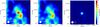 |
Fig. 1 Data reduction process for the LABOCA campaigns. All maps are zoomed to the innermost 3.5′× 3.5′. Left: a single measurement map of the GC from 2009-05-17T04:19:58. Center: model of the extended submm emission from the GC: co-added maps with subtracted point source at the position of Sgr A*. Right: remaining map for the 2009-05-17T04:19:58 map after subtraction of the GC model for the extended emission. The point like source represents the submm emission from Sgr A* itself. |
LABOCA is a multi-channel bolometer array, consisting of 295 channels, installed at the APEX telescope. APEX is a 12 m radio telescope located at the Llano de Chajnantor Observatory 50 km east of San Pedro de Atacama in northern Chile. It is situated at an altitude of 5014 m. LABOCA operates in the 345 GHz (870 μm) atmospheric window and has a bandwidth of 60 GHz. The beam shape can be described as a circular Gaussian with a full width half maximum (FWHM) ~ 19′′. For a detailed description of the observational process and data reduction we refer the reader to Eckart et al. (2008a,b). Here we only give a short overview:
The GC observations were performed using the On-the-fly (OTF) mapping technique with about 280 s integration time, map sizes of about 0.7°× 0.4°, with a fully sampled map2 of 0.5°× 0.17°. For different observations the position angle of the scan with respect to the Galactic plane was changed to average out artificial scanning effects. During observations in 2008 and 2009 we switched the angle between 10°, 0°and −10°; all other observing campaigns used a random angle between −47° and −17°. Furthermore, measurements of secondary calibrators (G10.62, IRAS 16293-2422) and skydips were carried out for different observations. Skydips allow to determine the opacity of the atmosphere as a function of elevation and secondary calibrators are close to the GC and therefore allow calibration with a minimum amount of telescope driving time.
Data reduction was done with the Bolometer Array Analysis Software (BoA, Schuller 2012). This involves the following steps: atmospheric correction, flat-fielding, de-spiking, (spatially correlated) sky noise removal, correlated instrumental noise removal and a correction for pointing offset. In the left panel of Fig. 1 we show a resulting GC map after having applied these corrections.
We present data obtained in a time span of seven years, with variable observing conditions. In this context one of the parameters that changes the most is the atmospheric opacity. With the LABOCA data there are three different options to estimate it: skydips3, radiometer values4, or a combination of both. It has been studied that opacities estimated with skydips tend to underestimate the flux density5, whereas those derived with the radiometer tend to overestimated it6. A weighted average of both radiometer and skydips gives an intermediate result that occasionally7 is better adjusted (A. Weiss, priv. comm.). We performed all three estimations for every observing night, and chose the technique that optimized the agreement between the secondary calibrator values as well as the individual maps and the co-added reference map (see below). The variations in respect with the corresponding reference values result in an estimate of the relative uncertainty in the light curve measurements of the order of 4% (1σ). After this initial step all good quality images of one campaign were co-added, in other words aligned, added and normalized to the total number of added images. A Gaussian point source was fit at the position of Sgr A*. This point source was subtracted from the co-added GC map leaving a model of the extended submm emission of the GC (Fig. 1, middle). Afterwards this model was subtracted from each individual map (Fig. 1, right). On the remaining flux density map again a Gaussian point source was fit at the position of Sgr A*. The peak of the Gaussian is supposed to yield the flux density of Sgr A* at the observation time. From all 8 LABOCA campaigns between 2008 and 2014 we obtained 24 light curves with a total of 792 data points.
2.1.2. Literature data
We extended the submm data set with archival data at comparable wavelengths (see Table 1). Though there is a small scatter in the observed central frequencies, in a good approximation all measurements can be treated equally. The difference between 850 and 890 μm is negligible (Fig. 1 in Marrone et al. 2006b). The literature datasets contain additional 345 data points in total. Thus the complete submm sample consists of 1137 flux density values. Figure 2 gives an overview of all used observations in the decade between 2004 and 2014.
Literature data used to extend the submm sample.
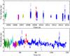 |
Fig. 2 Top: all available submm light curves between 2004 and 2014. The plot contains both the LABOCA data (blue circles) and the literature data (green down-pointing triangles: Eckart et al. 2009; cyan left-pointing triangles: Yusef-Zadeh et al. 2006a; magenta right-pointing triangles: Yusef-Zadeh et al. 2008; yellow squares: Yusef-Zadeh et al. 2009; red up-pointing triangles: Trap et al. 2011). Bottom: a concatenated light curve of the submm data. Time gaps greater than 10 min were replaced by gaps of 300 s. |
2.2. The radio data
To investigate the flux density distribution of Sagittarius A* in the radio regime we used data from the Australia Telescope Compact Array (ATCA) at a frequency of 100 GHz which are already published in Borkar et al. (2016). For more details about the observation campaigns and data reduction we refer the reader to their paper. Here we only give a brief overview.
ATCA is an array of six 22-m antennas of which five are available for 100 GHz observations. It is located at the Paul Wild Observatory, about 25 kilometers west of Narrabi in Australia and at an altitude of 234 m. Differential flux density light curves were collected for a total of 16 observation days during 2010 and 2014. Four observation days were excluded from our data set due to bad weather conditions.
As the antenna gain of ATCA is highly dependent on the elevation angle, calibrators within 10° from the GC were used (mainly PKS 1741-312 as a flux density and visibility calibrator). After each observation a flux density calibration was carried out using Uranus. Only observational data from elevations above 40° were processed. At smaller elevations gravitational deformation of the dishes, atmospheric effects and shadowing may lead to unreliable measurements. The observations were predominantly carried out in the H214 configuration with a maximum available baseline of 214 m. At a frequency of 100 GHz this corresponds to a synthesized beam of 2′′. For the GC observations this means, that the correlated flux densities on different baselines are dominated by the extended emission8 from the surroundings of Sgr A* on size scales of 20 to 30 arcesconds with peak flux density contributions at 100 GHz of the order of 0.1–0.2 Jy per beam; hence, the integrated values per baseline and hour angle are larger. To obtain the intrinsic variability of Sgr A* a method introduced by Kunneriath et al. (2010) was used (see also Borkar et al. 2016). Though the authors provide a formula for the time depend uncertainty of the differential flux density, δS(t), we took the median of these values,  Jy, as an estimate of the overall uncertainty.
The used Compact Array Broadband Backend (CABB) has an average time resolution of 10 s. As we do not expect intrinsic flux density variations at timescales below minutes (in Borkar et al. 2016 it is shown that the structure functions of the daily differential light curves are flat up to time lags of approximately 10 min), and to make the time resolution comparable to the LABOCA data, we averaged the differential flux density values over 300 s. Rough calculations have shown that the estimated distribution parameters (see Sect. 4) do not change significantly by averaging over timescales of up to several minutes9. The differential light curves contain both negative and positive values. To obtain the physically relevant value, namely the positive deviation from the quiescent state, we subtracted the lowest 10th percentile of the complete data set from the binned light curves. Finally we omitted all remaining negative flux density values. The original data sample contains 24 877 data points, after averaging and background subtraction we end up with 613 and 552 flux density values, respectively. A concatenated light curve of these values is shown in Fig. 3.
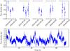 |
Fig. 3 Top: all ATCA 100 GHz light curves obtained between 2010 and 2014. The flux density values are averaged over a window of 300 s. Bottom: concatenated light curve of the averaged radio data after background reduction and removal of negative values. Time gaps greater than 10 min were replaced by gaps of 300 s. |
3. Statistical analysis of the submm flux density distribution
For the distribution analysis of the submm (and later also the radio) light curves we assume that all single flux density measurements can be treated as interchangeable random values. While this is not strictly true for short time scales (flux density values within distinct flaring events follow a temporal sequence typically of the order of one hour), these correlations disappear on larger time scales of the order of days or even years (Yusef-Zadeh et al. 2011; Dexter et al. 2014; Bower et al. 2015). Thus, for a long-term analysis all flux density values can be handled in a good approximation as uncorrelated stochastic variables.
To get a first impression of the underlying distribution several methods of visualizing the data can be considered. A common way is to create a histogram of the flux density values. Histograms though face the problem of properly binning the data, which is connected to additional analytic challenges (e.g., Knuth 2006 or Shimazaki & Shinomoto 2007). If the number of bins is chosen too large, a histogram will overemphasize statistical fluctuations, while a too small number of bins may cause a loss of information of the underlying data structure. Without going into detail we used the algorithm introduced in Knuth (2006) to determine the optimal number of bins for the data sets, yielding 17 bins for the submm data (Fig. 4) and later seven bins for the radio data (Sect. 4). For the logarithms of the submm and radio data used in log-log histograms the optimal number of bins computes to 16 and ten, respectively.
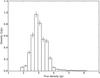 |
Fig. 4 Histogram of the submm flux density values. The steady quiescent emission leads to the average of ~3 Jy, the high-flux tail up to ~6 Jy is supposedly power-law distributed. |
3.1. Modeling a power-law distribution
We begin the flux density distribution analysis by introducing some basic definitions and considerations about power-law distributions. The probability density function (PDF) of a power-law distributed variable can be written as 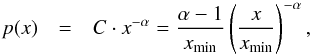 (1)where xmin is the domain’s lower bound, α the power-law index and
  the normalization constant. The cumulative distribution function (CDF) is then given by
 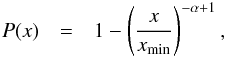 (2)with the survival function or complementary cumulative distribution function (CCDF)
 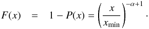 (3)A commonly used indicator for an underlying power-law is a linear behavior of the empirical PDF or CCDF tail in a log-log plot with log p(x) ∝ − αlog x. The slope of this graph then indicates the power-law index α.
If we now consider a power-law with a constant shift s, for instance a red noise emission process superimposed with a steady quiescent contribution, the form of the power-law changes to what we call a shifted power-law: 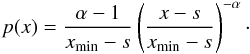 (4)In a log-log view, a shifted power-law does not show the linear behavior unless for large values of x, as
  (5)The second term at the right-hand side of Eq. (5)leads to a curvature in a log-log plot as shown in Fig. 5. This term is determined by the ratio between quiescent and flaring emission and therefore is crucial particularly for the analysis of the submm flux density distribution. Only for x ≫ s ⇒ s/x → 0 the slope converges to α. If we consider a steady quiescent submm emission of about 3 Jy and flaring peaks of up to 6 Jy (Fig. 4), we expect s/x-ratios of about 0.5 or higher. That implies, that even if the variable radiation is generated by a power-law distributed process, the steady quiescent emission causes a curvature in a logarithmic probability plot. This might lead to a premature rejection of a power-law hypothesis or a broken power-law conjecture. Figure 6 shows a log-log histogram of the submm data. A negative curvature in the histogram’s high-flux tail ≳3.5 Jy is visible. Therefore, the challenge for the submm analysis is to separate the quiescent from the variable flaring emission. In the following sections we present two methods of doing so:
-
A heuristic method, which is based on physical and observationalconsiderations (Sect. 3.2). After havingsubtracted a heuristic model for the quiescent emission from thelight curve, the remaining flux density sample can be tested for anunshifted power-law distribution (Sect. 3.3) as inEq. (1).
-
A numerical method (Sect. 3.4) which is based on Eq. (4)(a shifted power-law) and contains a mathematical estimator for the quiescent emission, s.
The analysis of the radio data (Sect. 4) copes without the additional estimator s as the method of taking differential light curves already inherently includes the subtraction of a quiescent contribution.
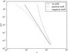 |
Fig. 5 PDFs for shifted power-laws (α = 12, xmin = 3.5) with different shifts, solid line without shift, dashed line with positive, dash-dot line with negative shift. The slope only becomes constant for large x. |
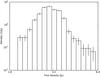 |
Fig. 6 log-log histogram of the submm data. The curvature of the high-flux tail ≳ 3.5 Jy indicates a shifted power-law of the form p(x) ~ (x − s)α. |
3.2. Heuristic estimation of the quiescent submm emission
Possible estimators for the quiescent radiation can be found by simple heuristic considerations. For instance, our submm sample spans a flux density range from about 2 Jy to 6 Jy. Thus, as a lowest bound for an estimator we may just take the lowest 1st percentile of the sample (~2 Jy). This can be seen as the lowest possible quiescent baseline. An upper limit for a constant estimator is the 50th percentile (median, ~3 Jy). This value is based on the idea, that if all radiation stems from one quiescent process, meaning that the variable emission is negligible, the median flux density value is a good estimator for the most probable flux density value. If we now consider two combined emission processes, one quiescent process and a flaring activity, the median surely is the upper limit for the quiescent emission estimator. However, this constant estimator s may take all values between the 1st and the 50th percentile.
Another consideration can be given to the temporal development of the quiescent emission: though long term observations of Sgr A* have shown, that on time scales above days no periodicities can be found (Dexter et al. 2014), the possibility of long term variations can not completely be ruled out (Pierce-Price et al. 2003). Therefore we have to consider a possible change in the quiescent emission over longer timescales. As no further information about a putative temporal development of the quiescent flux density distribution is available, we used three simplistic models for the long term variability: a linear trend, a constant quiescent level per each observing campaign and a third polynomial order trend modeled by a cubic spline. In summary, we define 4 models, which may possibly represent the steady quiescent emission:
-
A
Constant quiescent flux density contribution(Fig. 7): we assumed a constant low-fluxcontribution yielding a global estimator s for the quiescent emission. As possible values for s we took the range of the [ 1,5,10,30,50 ]th percentile of the flux density values.
-
B
Quiescent flux density contribution with linear trend (Fig. 8): we calculated the mean flux density value for each observing campaign. A trend line was fit to these values, the difference between the trend line and the global mean was subtracted from the light curves. After having detrended the data a global value for the quiescent emission was assumed (according to the model described in A).
-
C
Non-parametric variable quiescent flux density contribution (Fig. 9): we supposed a long term variability in the quiescent emission without assuming a parametric equation. Instead, for each observing campaign we took the lowest nth ([ 1,5,10,30,50 ]th) percentile. To not overestimate outliers we introduced a threshold of 30 data points per campaign. If an campaign contains less data we calculated the quiescent emission’s value by a linear interpolation of the two neighboring campaigns.
-
D
Variable quiescent flux density contribution modeled by a cubic spline (Fig. 10): we modeled the variability in the quiescent emission with a third order polynomial. The nth percentile of each campaign was calculated and a cubic spline fit was performed on these values.
The resulting models were then subtracted from the observed light curves to obtain the variable emission.
3.3. Fitting the variable submm emission
We used a distribution fitting formalism which has been introduced by Clauset et al. (2007), hereinafter CSN07. This formalism is briefly summarized in Appendix A. We point out, that the CSN07 algorithm is only applicable to unshifted power-laws, meaning that it only yields estimators for xmin and α, not for a possible shift s. Thus we had to subtract the quiescent emission using the heuristic methology described in Sect. 3.2 and fit the remaining dataset with a power-law model. The results of this procedure are summarized in Table 2.
If we choose a significance level of 0.05, some power-law fits have to be rejected due to their low p-value (see Appendix A). The corresponding data set is unlikely power-law distributed. Although we note that higher p-values can not be used for model verification, we can nevertheless formulate the results as follows: we found some heuristic models for the quiescent emission which yield, after subtraction, high flux density samples that can be described by power-law distributions. The power-law distribution fits yield a range of best estimators for α and xmin: ![Mathematical equation: \begin{eqnarray} &&\alpha \in [(3.3\pm0.3),(6.9\pm0.7)]\,\mathrm{and}\\ &&x_{\mathrm{min}} \in [(0.46\pm0.07),(1.50\pm0.08)]\mathrm{Jy}. \end{eqnarray}](/articles/aa/full_html/2017/05/aa28530-16/aa28530-16-eq48.png) The mean of the obtained parameters from all non rejected fits is
The mean of the obtained parameters from all non rejected fits is (8)The statistical meaning of Eq. (8)might be weak, as the different fits were performed on different data sets. Though it gives an impression of the numerical size of α and xmin.
In Table 2 we also include a column with a new parameter x∗min. Before we applied a power-law fitting routine we subtracted different models for the unknown quiescent emission from the original sample. Thus, the resulting xmin is the flux density value where the power-law begins for the data where the quiescent emission has been subtracted. Instead x∗min indicates where the power-law tail starts in the original sample. Hence, from an observer’s perspective, x∗min is the more interesting parameter. To obtain this value, the estimator for xmin needs to be re-shifted again, such that x∗min = xmin + s. For models C and D we added a single value s although we had subtracted a function for the quiescent radiation (i.e., a per campaign value and a cubic spline). As the different values for x∗min mostly serve for consistency comparison, a decent approximation for this re-shifting is to take the nth percentile from the original data (depending on the percentile parameter we used in the corresponding model) and add this value to the calculated xmin. For model B we added the nth percentile of the detrended data. This method yields only rough estimates for x∗min, and thus we omit uncertainty considerations.
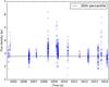 |
Fig. 7 Quiescent emission model A: subtraction of a constant contribution from the data. In this example the steady contribution is the lowest 30th percentile of all data points. |
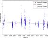 |
Fig. 8 Quiescent emission model B: linear detrending, followed by the subtraction of a global constant for the quiescent emission (not depicted in this plot). |
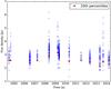 |
Fig. 9 Quiescent emission model C: subtraction of a variable quiescent emission. In this example for each campaign the 10th percentiles of the campaign’s data is subtracted. |
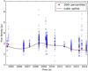 |
Fig. 10 Quiescent emission model D: the variable quiescent emission is modeled by a cubic spline. Here the spline fit is applied to the 20th percentile values of each campaign. |
3.4. Numerical estimation of the quiescent and variable submm emission
In the previous section we analyzed the submm flux density distribution by introducing several heuristic models for the non-flaring, quiescent emission of Sgr A*. We subtracted these models from the measured data sets and performed a power-law hypothesis test according to CSN07 on the remaining data. Under the assumption of a constant quiescent contribution it is also possible to numerically obtain an estimator s for the quiescent emission out of the given data set. This method was proposed by RKE09. We briefly describe the fitting procedure in the following:
As we have already discussed in Sect. 3.1, a quiescent contribution to a power-law process leads to a curvature in a log-log representation of the flux density distribution (Fig. 5 and Eq. (4)). RKE09 inverse the argument, such as the curvature of such a plot is vice versa a direct mathematical indicator for the unknown power-law shift s. That is, in this context, the steady quiescent emission. The estimator for s can be found by straightening out the log-log plot through adding an appropriate constant to the flux density distribution. The constant, that minimizes the deviation from a best linear fit is an estimator s for the steady shift of the power-law. Once we obtained s, it is possible to test the sample for a shifted power-law hypothesis. The resulting fitting procedure for a shifted power-law according to RKE09 can briefly be described as follows:
-
Sort the elements of the data set: { X1,...,XN } →
 with x1 ≤ ... ≤ xN.
 -
For each value xi in
 assume it to be xmin (i.e., xi = xmin,i) and create a new ordered data set
  .
. -
For each possible value sj in a given shift range { smin,...,smax } shift
 with sj:
  . For the possible shift range we assume the range between −5 and 5 Jy with iteration steps of 0.1 Jy.
 -
For each
 calculate the empirical survival function
  (see Eq. (A.4)) and do a linear fit in a log-log representation.
 -
The value sj that minimizes the R2-value of the linear fit, is the shift estimator si for a given xmin,i.
-
Shift the data set with the shift estimator si:
 and calculate the Hill estimator for αi (see Eq. (A.3)) with
  .
. -
For each xmin,i calculate the KS-distance D between the empirical survival function
 (see Eq. (A.4)) and the theoretical survival function
  with αi, si and xmin,i:
  (9)For a shifted power-law, F(x) is given by
  (10)
(10) -
As best fit accept the estimators xmin,i, si and αi which minimize the parameter D.
-
Error estimations and a goodness of fit value are obtained by the bootstrapping techniques described in Appendix A.
Applying this method to the submm sample yields the shifted power-law parameters: (11)with a p-value of 0.53.
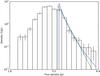 |
Fig. 11 log-log histogram of the submm flux density with shifted power-law fit (blue line) from the RKE09 algorithm and a pure power-law fit (green line) according to CSN07. The obtained power-law indices for the RKE09 and CSN07 method are α~4 and ~ 12, respectively. |
Figure 11 demonstrates the difference between both power-law fitting methods we presented: the CSN07 algorithm fits an unshifted power-laws without the additional parameter s, so the fit in the log-log plot will always be linear. The shown fit corresponds to the first row in Table 2. The RKE09 fitting procedure can reproduce the internal shift by a quiescent contribution which is manifested as the curvature of the probability density distribution. Although both fits look similar, the resulting power-law indices are very different.
In Table 3 we compare the mean results (Eq. (8)) from Sect. 3.3 (I) with the results from the RKE09 method (II) from this section. Within uncertainties, both results appear to be in agreement and suggest, that the power-law index α is consistent with a value of four. Moreover we compare the RKE09 results to a specific model from Sect. 3.3: model A (a constant quiescent emission) with a percentile parameter of 30% (III). This percentile parameter corresponds to a value of 2.79 Jy. The motivation for comparing the RKE09 with this specific model is the following: although we have considered different models for a varying quiescent emission (models B–D), the simplest model (a constant quiescent emission) should always be preferred until observational evidence demands for more complexity (e.g., a significant detection of long-term periodicities in the quiescent emission). The fact that applying a CSN07 fit to this specific model is in good agreement with the RKE09 results primarily only shows, that both fitting approaches yield unbiased estimators and work accordingly. Moreover, we are able to suggest a statistical model of the submm emission which is both heuristically and analytically consistent: a power-law with an intrinsic lower bound ~0.6 Jy10 and an index α~ 4 which is superimposed by a constant quiescent emission with an average flux density of about 2.8 Jy. Though, if more complexity is demanded in the modeling of the quiescent emission, we have also shown that the results for the submm emission model do not change significantly. In the later discussion we refer to the parameters found with the RKE09 method as we deem this the superior approach.
Comparison of the results for the submm data from parameter estimation approaches.
4. Statistical analysis of the radio flux density distribution
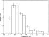 |
Fig. 12 Histogram of the 100 GHz flux density values. |
The results from the previous section show, that the variable submm emission can be described by a power-law with an index of about four. A power-law analysis of the 100 GHz ATCA data (shown in a histogram in Fig. 12) can be done accordingly. With the introduced methods (CSN07 and RKE09) power-law distributions in differential light curves (the ATCA radio data) and in light curves with absolute flux density values (the submm data) can directly be compared. In differential light curves the quiescent emission is already pre-subtracted; hence a pure power-law (CSN07) can be assumed. Absolute light curves may additionally contain the quiescent emission, so that a shift estimator has to be included (RKE09). Thereby, the RKE09 estimator for the power-law index α is shift invariant. Thus, the fitting algorithm of CSN07 for pure power-laws can be applied to the ATCA data and the submm and radio power-law indices can directly be compared. For the 100 GHz data we find as best fit parameters10 (12)with a p-value of 0.08. To check for consistency we also perform a fit based on the RKE09 method. Table 4 shows, that the results from both fitting techniques are in good agreement. Figure 13 depicts a log-log histogram with both the best unshifted (CSN07) and shifted (RKE09) power-law fit. Within uncertainties, the power-law index is consistent with the one found in the NIR and submm distributions, namely approximately four.
Comparison of the results (for the radio data) from the CSN07 fitting method (I) to the results from the RKE09 algorithm (II).
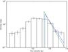 |
Fig. 13 log-log histogram of the radio flux density with power-law fits. Both the CSN07 (green line) and the RKE09 (blue line) method yield similar fits, the power-law slopes are within uncertainties consistent with α ~ 4. |
5. Consequences for the model of adiabatically expanding blobs
The fact that at 100 GHz and 350 GHz we find power-law flux density distributions with exponents α ~ 4.0 suggests that the (sub)mm- and NIR-flares are linked to each other and have the same origin. Witzel et al. (2012) find in the NIR a power-law with α = 4.2 ± 0.1. Under the assumption that the NIR spectra are the optically thin extension of the submm flare component spectra, a different flux density distribution in the submm domain than a power-law would be inconsistent with the NIR measurements. The similar nominal value of the power-law indices at different wavebands (mm, submm and NIR) can also put additional constraints on the model of adiabatically expanding self-absorbed synchrotron blobs:
Previous measurements have already suggested that contributions from flares with initial turnover frequencies below 100 GHz are less likely as the variability drops toward lower frequencies (see Sect. 1 and references therein). A significant population of flares peaking at or below 100 Hz would contradict this trend. A substantial contribution from flares peaking between 100 GHz and 350 GHz has the same problem. Flares with initial turnover frequencies well above 350 GHz are also probably rare as the overall spectrum drops strongly toward the far-infrared in the frequency range of 300–400 GHz (Marrone et al. 2006a,b; Marrone 2006; Eckart et al. 2012). In the following we investigate this formaly.
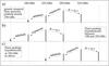 |
Fig. 14 Schematic representation of possible peak contributions to different frequency channels from different temporal spectra of adiabatically expanding flares. |
In Fig. 14 we show a schematic representation of possible peak contributions to different frequency channels from different temporal spectra of adiabatically expanding flares. With respect to the peak frequency, contributions to higher frequencies are due to the optically thin synchrotron part of the contaminating flare component spectrum. In the (sub)mm domain flare components of Sgr A* have not yet been isolated spectrally or spatially. As we are only considering frequently observed strong flares with amplitudes between a few tenths and a few Janskys, we assume that the optically thin synchrotron spectral index is also close to the one measured in the infrared, that is around αsync = − 0.7. Steeper spectral indices in the NIR wavelength domain are most likely due to synchrotron losses and do not reflect the intrinsic optically thin spectral index (see Bremer et al. 2011 and Witzel et al. 2014 for details).
Contributions to lower frequencies are mainly due to the adiabatic expansion process. Low frequency contributions due to the optically thick part of the synchrotron components are not considered as the spectrum there rises with a very steep index of ~+2.5. In Fig. 14a we show a generic temporal spectrum peaking around 350 GHz. In Fig. 14b we show the case of a spectrum peaking between 100 GHz and 350 GHz. The optically thin synchrotron spectrum and the adiabatic expansion process result in contributions at the neighboring frequencies. In Fig. 14c we show the case of a spectrum peaking above 350 GHz. Here, only the adiabatic expansion process results in contributions at the lower frequencies. In case of the presence of contaminating flares like the ones shown in Fig. 14bc their contribution should be added to the generic flare spectrum peaking at 350 GHz as shown in Fig. 14a. In both cases the contaminating flares below and above 350 GHz contribute to the high or low end of the flux density distribution at 100 GHz and 350 GHz.
In the following we use the concept of Fig. 14 to quantify the effect the contaminating flare populations have on the flux density power-law index of the generic flare spectrum shown in Fig. 14a. We use D to denote the dynamic range, defined as the ratio between brightest and faintest (significant) flare fluxes that contribute to the power-law section of the flux density histogram. The flux densities are corrected for the constant s by which the power-law has been shifted and normalized to unity by division by xmin. The frequencies of occurrence are also normalized (so that highest frequency becomes unity). From our (sub)mm-light curves we find D in the range of ~2.5–5. Then the frequencies of flare amplitudes at the low and high end of the power-law part of the distribution are unity and P and the power-law index α is defined as:  (13)Here the frequencies and dynamic range values can now be modified according to the situations at the different observing wavebands resulting in power-law indices for the simple extreme cases. If we assume that the nominal value of the power-law index of our generic (sub)mm-flare spectrum peaking at 350 GHz is the same as the index α = −4.2 found in the NIR, one can show that the corresponding power-law index of the contaminated flare flux density spectrum can be described via
  (14)Here, R is the factor by which the flux density frequency is increased due to the contamination, which means that R = 2 for a 100% additional contribution from contaminating flares. The varying operation signs reflect that the index can be lowered or enlarged depending on whether the faint of bright end of the distribution is enhanced. As a result we find that with the current typical uncertainty in the power-law index in the (sub)mm- regime around Δα = 1, we can only exclude contamination flare flux contributions that increase the flux density frequencies by a factor of about 5. However, if we assume an intrinsic power-law index equals that found in the NIR and the power-law index uncertainty that is not larger than the value Δα = ± 0.1 derived from the NIR, then the contaminating contributions to the uncontaminated flux density frequencies at 100 GHz and 350 GHz of around 15% to 20% can be excluded. This assumption implies that the measured difference between the submm and the radio power-law indices and the NIR power-law index are entirely due to measurement uncertainties and (currently) smaller statistics in the submm and radio domain. This then supports the picture, that most of the flares are indeed borne within the 300–400 GHz domain and are to first order of similar nature consistent with the spectral index and power-law distribution index information found in the NIR and the (sub)mm domain.
Accepting that the bulk of observed flares have the same origin and initially peak at ~350 GHz and above, consequences for the possible expansion velocity of the adiabatic expansion can be inferred: according to van der Laan (1966) the peak frequency, νm, decreases as: 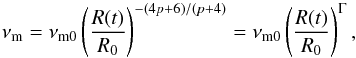 (15)where p is the power-law index of the energy spectrum of the synchrotron emitting electrons with n(E) ∝ E− p, νm0 the initial peak frequency, R0 the initial source size and R(t) the source size after the expansion time t. R(t) can be modeled by linear expansion at constant expansion speed, vexp, as
 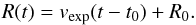 (16)If one again assumes the measured NIR spectral information, namely p = 2αsync + 1 ≈ 2.4 with the synchrotron spectral index αsync, as also being valid for the (sub)mm flares, the exponent Γ of the right-hand side of Eq. (15)becomes ≈− 2.44. Therefore
 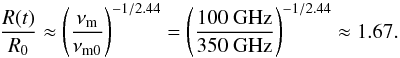 (17)We note that Eq. (17)is only mildly sensitive to p. If one assumes extreme cases, such as p in the range between 1 and 9 (e.g., Yusef-Zadeh et al. 2006a or Hornstein et al. 2007), the normalized expansion radius R(t) /R0 would range from 1.87 to 1.47, and thus the result would deviate only by ~10%.
Using Eqs. (15)and (16)the time delay t4 − t3 between peaks at two arbitrary frequencies ν4 and ν3 can be calculated if the time lag t2 − t1 between peaks at two frequencies ν2 and ν1 is known: 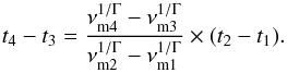 (18)Yusef-Zadeh et al. (2006b, 2008) found time delays between peaks at 44 and 23 GHz to be ~0.5 h, in Brinkerink et al. (2015) the time lag between a peak at 100 and 19 GHz was measured as ~1.1 h. Thus, typical time delays between peaks at 350 GHz and 100 GH are expected to be ~0.5 h. Therefore, using Eqs. (16)and (17), we get
 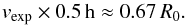 (19)R0 can additionally be constrained to be of a typical size scale of the order of 1 Schwarzschild radius (RS) (Doeleman et al. 2009; Fish et al. 2011; García-Marín et al. 2011; Eckart et al. 2012). Hence,
 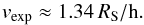 (20)For Sgr A* an expansion velocity of 1 c corresponds to about 100 RS per hour. If one introduces the terms fast, intermediate and slow expanding synchrotron blobs for expansion velocities of 0.1, 0.01 and 0.001 c, respectively, it can be seen that under the aforementioned assumptions the bulk of observed flares expand at intermediate velocities, meaning that vexp ~ 0.01 c. Fast and slow expansion velocities would require initial blob sizes R0 of the order of 10 and 0.1 RS, respectively.
6. Conclusions
We compiled both submm light curves obtained mainly from LABOCA observation campaigns extended with literature data and 100 GHz radio data from observations carried out with ATCA. Having investigated these data sets we found that the variable flux density distribution for both wavelength regimes are well described by a single state power-law distributed emission process with a power-law index α~ 4. This finding may put general constraints on any emission model for the observed flares of Sgr A*. The fact, that the NIR flaring emission follows the same distribution can be seen as an additional indicator that the radio, submm and NIR variability stem from the same source components. This has already been predicted by the model of adiabatically expanding synchrotron blobs, which is capable to fit simultaneous multi-wavelength light curves. Our statistical findings may strengthen this model. A situation, where the radio, submm and NIR emissions stem from different source components or even different mechanisms and are describable by the same flux density distribution is possible though, but unlikely.
Inside the framework of a model of adiabatically expanding synchrotron blobs we may also conclude, that the initial turnover frequencies ν0 of the synchrotron sources are predominantly around 350 GHz. Otherwise the radio flux density distribution would either yield a significantly different power-law index than approximately four or be a completely different distribution. Moreover, the conclusion that the bulk of observed flares are of similar nature may also infer an average expansion velocity of the synchrotron blobs of the order of ~0.01 c.
This can be derived from polarization measurements of flare emission (Eckart et al. 2007; Marrone et al. 2008).
No measurement gap larger than half of the beamwidth.
By measuring the emission of the atmosphere as a function of elevation, proportional to (1 − e− τ), the atmospheric opacity τ can be determined.
Measuring a water line intensity with a water vapor radiometer the precipitable water vapor column density along the line of sight (and therefore the atmospheric opacity τ) can be determined.
Skydips are usually taken under good weather conditions whereas the conditions for the measurements may be less preferential.
Positive biases toward the detection of precipitable water overestimates the opacity.
For instance if the weather conditions differ in both directions from average conditions under which the calibration was done; using a weighted average is less susceptible to excursions in the weather conditions.
For a detailed discussion of the extended mm emission from the inner few parsecs of the GC we refer to Kunneriath et al. (2012) and Moser et al. (2017).
For example we performed a power-law fit with the later introduced CSN07 method to differently averaged data sets. The obtained estimator α = 4.7 for the power-law index is stable up to an averaging over 7 min and only slightly diverges to higher values, for instance 5.0 for an average over 10 min.
As explained in Appendix B the real value for xmin might indeed be smaller if one considers the possible influence of uncertainties (uncertainties in the light curves, variability in the quiescent emission, etc.). The value for α, which is the parameter from which we later draw conclusions, is not effected by these uncertainties though.
Acknowledgments
We received funding from the European Union Seventh Framework Program (FP7/2007–2013) under grant agreement No. 312789 – Strong gravity: Probing Strong Gravity by Black Holes Across the Range of Masses. This work was supported in part by the Deutsche Forschungsgemeinschaft (DFG) via the Cologne Bonn Graduate School (BCGS), the Max Planck Society through the International Max Planck Research School (IMPRS) for Astronomy and Astrophysics, as well as special funds through the University of Cologne and SFB 956 – Conditions and Impact of Star Formation. Part of this work was supported by fruitful discussions with members of the European Union funded COST Action MP0905: Black Holes in a Violent Universe and the Czech Science Foundation – DFG collaboration (No. 13-00070J).
References
- Baganoff, F. K., Maeda, Y., Morris, M., et al. 2003, ApJ, 591, 891 [NASA ADS] [CrossRef] [Google Scholar]
- Balick, B., & Brown, R. L. 1974, ApJ, 194, 265 [NASA ADS] [CrossRef] [Google Scholar]
- Borkar, A., Eckart, A., Straubmeier, C., et al. 2016, MNRAS, 458, 2336 [NASA ADS] [CrossRef] [Google Scholar]
- Bower, G. C., Markoff, S., Dexter, J., et al. 2015, ApJ, 802, 69 [NASA ADS] [CrossRef] [Google Scholar]
- Bremer, M., Witzel, G., Eckart, A., et al. 2011, A&A, 532, A26 [NASA ADS] [CrossRef] [EDP Sciences] [Google Scholar]
- Brinkerink, C. D., Falcke, H., Law, C. J., et al. 2015, A&A, 576, A41 [NASA ADS] [CrossRef] [EDP Sciences] [Google Scholar]
- Broderick, A. E., & Loeb, A. 2006, MNRAS, 367, 905 [NASA ADS] [CrossRef] [Google Scholar]
- Chan, C.-k., Psaltis, D., Özel, F., et al. 2015, ApJ, 812, 103 [NASA ADS] [CrossRef] [Google Scholar]
- Clauset, A., Rohilla Shalizi, C., & Newman, M. E. J. 2007, ArXiv e-prints [arXiv:0706.1062] [Google Scholar]
- Dexter, J., & Fragile, P. C. 2013, MNRAS, 432, 2252 [NASA ADS] [CrossRef] [Google Scholar]
- Dexter, J., Kelly, B., Bower, G. C., et al. 2014, MNRAS, 442, 2797 [NASA ADS] [CrossRef] [Google Scholar]
- Dodds-Eden, K., Porquet, D., Trap, G., et al. 2009, ApJ, 698, 676 [NASA ADS] [CrossRef] [Google Scholar]
- Doeleman, S. S., Fish, V. L., Broderick, A. E., Loeb, A., & Rogers, A. E. E. 2009, ApJ, 695, 59 [NASA ADS] [CrossRef] [Google Scholar]
- Eckart, A., & Genzel, R. 1996, in The Galactic Center, ed. R. Gredel, ASP Conf. Ser., 102, 196 [NASA ADS] [Google Scholar]
- Eckart, A., Schödel, R., Meyer, L., et al. 2007, in Black Holes from Stars to Galaxies – Across the Range of Masses, eds. V. Karas, & G. Matt, IAU Symp., 238, 181 [Google Scholar]
- Eckart, A., Baganoff, F. K., Zamaninasab, M., et al. 2008a, A&A, 479, 625 [NASA ADS] [CrossRef] [EDP Sciences] [Google Scholar]
- Eckart, A., Schödel, R., García-Marín, M., et al. 2008b, A&A, 492, 337 [NASA ADS] [CrossRef] [EDP Sciences] [Google Scholar]
- Eckart, A., Baganoff, F. K., Morris, M. R., et al. 2009, A&A, 500, 935 [NASA ADS] [CrossRef] [EDP Sciences] [Google Scholar]
- Eckart, A., García-Marín, M., Vogel, S., et al. 2012, A&A, 537, A52 [NASA ADS] [CrossRef] [EDP Sciences] [Google Scholar]
- Falcke, H. 1999, in The Central Parsecs of the Galaxy, eds. H. Falcke, A. Cotera, W. J. Duschl, F. Melia, & M. J. Rieke, ASP Conf. Ser., 186, 113 [Google Scholar]
- Falcke, H., Goss, W. M., Matsuo, H., et al. 1998, ApJ, 499, 731 [NASA ADS] [CrossRef] [Google Scholar]
- Falcke, H., Markoff, S., & Bower, G. C. 2009, A&A, 496, 77 [NASA ADS] [CrossRef] [EDP Sciences] [Google Scholar]
- Fish, V. L., Doeleman, S. S., Beaudoin, C., et al. 2011, ApJ, 727, L36 [NASA ADS] [CrossRef] [Google Scholar]
- García-Marín, M., Eckart, A., Weiss, A., et al. 2011, ApJ, 738, 158 [NASA ADS] [CrossRef] [Google Scholar]
- Genzel, R. 2000, in Astronomische Gesellschaft Meeting Abstracts, ed. R. E. Schielicke, 16 [Google Scholar]
- Genzel, R., Schödel, R., Ott, T., et al. 2003, Nature, 425, 934 [CrossRef] [PubMed] [Google Scholar]
- Ghez, A. M., Wright, S. A., Matthews, K., et al. 2004, ApJ, 601, L159 [CrossRef] [Google Scholar]
- Herrnstein, R. M., Zhao, J.-H., Bower, G. C., & Goss, W. M. 2004, AJ, 127, 3399 [NASA ADS] [CrossRef] [Google Scholar]
- Hill, B. M., et al. 1975, Ann. Stats., 3, 1163 [CrossRef] [Google Scholar]
- Hornstein, S. D., Ghez, A. M., Tanner, A., et al. 2002, ApJ, 577, L9 [NASA ADS] [CrossRef] [Google Scholar]
- Hornstein, S. D., Matthews, K., Ghez, A. M., et al. 2007, ApJ, 667, 900 [NASA ADS] [CrossRef] [Google Scholar]
- Knuth, K. H. 2006, ArXiv Physics e-prints [arXiv:physics/0605197] [Google Scholar]
- Kunneriath, D., Witzel, G., Eckart, A., et al. 2010, A&A, 517, A46 [NASA ADS] [CrossRef] [EDP Sciences] [Google Scholar]
- Kunneriath, D., Eckart, A., Vogel, S. N., et al. 2012, A&A, 538, A127 [CrossRef] [EDP Sciences] [Google Scholar]
- Li, Y.-P., Yuan, F., Yuan, Q., et al. 2015, ApJ, 810, 19 [NASA ADS] [CrossRef] [Google Scholar]
- Marrone, D. P. 2006, Ph.D. Thesis, Harvard University, USA [Google Scholar]
- Marrone, D. P., Moran, J. M., Zhao, J.-H., & Rao, R. 2006a, ApJ, 640, 308 [NASA ADS] [CrossRef] [Google Scholar]
- Marrone, D. P., Moran, J. M., Zhao, J.-H., & Rao, R. 2006b, J. Phys. Conf. Ser., 54, 354 [Google Scholar]
- Marrone, D. P., Baganoff, F. K., Morris, M. R., et al. 2008, ApJ, 682, 373 [NASA ADS] [CrossRef] [Google Scholar]
- Marscher, A. P. 1983, ApJ, 264, 296 [NASA ADS] [CrossRef] [Google Scholar]
- Moser, L., Sánchez-Monge, Á., Eckart, A., et al. 2017, A&A, in press DOI: 10.1051/0004-6361/201628385 [Google Scholar]
- Neilsen, J., Nowak, M. A., Gammie, C., et al. 2014, in The Galactic Center: Feeding and Feedback in a Normal Galactic Nucleus, eds. L. O. Sjouwerman, C. C. Lang, & J. Ott, IAU Symp., 303, 374 [Google Scholar]
- Pierce-Price, D., Jenness, T., Richer, J., & Greaves, J. 2003, Astron. Nachr. Suppl., 324, 413 [NASA ADS] [CrossRef] [Google Scholar]
- Porquet, D., Predehl, P., Aschenbach, B., et al. 2003, A&A, 407, L17 [NASA ADS] [CrossRef] [EDP Sciences] [Google Scholar]
- Quataert, E. 2002, ApJ, 575, 855 [NASA ADS] [CrossRef] [Google Scholar]
- Rácz, É., Kertész, J., & Eisler, Z. 2009, ArXiv e-prints [arXiv:0905.3096] [Google Scholar]
- Sabha, N., Witzel, G., Eckart, A., et al. 2010, A&A, 512, A2 [NASA ADS] [CrossRef] [EDP Sciences] [Google Scholar]
- Schödel, R., Ott, T., Genzel, R., et al. 2002, Nature, 419, 694 [NASA ADS] [CrossRef] [PubMed] [Google Scholar]
- Schuller, F. 2012, in SPIE Conf. Ser., 8452, 1 [Google Scholar]
- Shahzamanian, B., Eckart, A., Valencia-S., M., et al. 2015, A&A, 576, A20 [NASA ADS] [CrossRef] [EDP Sciences] [Google Scholar]
- Shimazaki, H., & Shinomoto, S. 2007, Neural computation, 19, 1503 [Google Scholar]
- Siringo, G., Kreysa, E., Kovács, A., et al. 2009, A&A, 497, 945 [NASA ADS] [CrossRef] [EDP Sciences] [Google Scholar]
- Tagger, M., & Melia, F. 2006, ApJ, 636, L33 [NASA ADS] [CrossRef] [Google Scholar]
- Trap, G., Goldwurm, A., Dodds-Eden, K., et al. 2011, A&A, 528, A140 [NASA ADS] [CrossRef] [EDP Sciences] [Google Scholar]
- Trippe, S., Gillessen, S., Ott, T., et al. 2006, J. Phys. Conf. Ser., 54, 288 [CrossRef] [Google Scholar]
- van der Laan, H. 1966, Nature, 211, 1131 [NASA ADS] [CrossRef] [Google Scholar]
- Witzel, G., Eckart, A., Bremer, M., et al. 2012, ApJS, 203, 18 [NASA ADS] [CrossRef] [Google Scholar]
- Witzel, G., Morris, M., Ghez, A., et al. 2014, in The Galactic Center: Feeding and Feedback in a Normal Galactic Nucleus, eds. L. O. Sjouwerman, C. C. Lang, & J. Ott, IAU Symp., 303, 274 [Google Scholar]
- Yusef-Zadeh, F., Bushouse, H., Dowell, C. D., et al. 2006a, ApJ, 644, 198 [NASA ADS] [CrossRef] [Google Scholar]
- Yusef-Zadeh, F., Roberts, D., Wardle, M., Heinke, C. O., & Bower, G. C. 2006b, ApJ, 650, 189 [NASA ADS] [CrossRef] [Google Scholar]
- Yusef-Zadeh, F., Wardle, M., Heinke, C., et al. 2008, ApJ, 682, 361 [NASA ADS] [CrossRef] [Google Scholar]
- Yusef-Zadeh, F., Bushouse, H., Wardle, M., et al. 2009, ApJ, 706, 348 [NASA ADS] [CrossRef] [Google Scholar]
- Yusef-Zadeh, F., Miller-Jones, J., Roberts, D., et al. 2011, in The Galactic Center: a Window to the Nuclear Environment of Disk Galaxies, eds. M. R. Morris, Q. D. Wang, & F. Yuan, ASP Conf. Ser., 439, 285 [Google Scholar]
- Zubovas, K., Nayakshin, S., & Markoff, S. 2012, MNRAS, 421, 1315 [NASA ADS] [CrossRef] [Google Scholar]
Appendix A: Power law fitting: the Clauset algorithm (CSN07)
The likelihood function of a power-law is given by 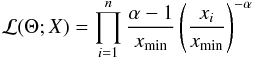 (A.1)with Θ as free parameters, here xmin and α.
The logarithm of the likelihood function is then given by 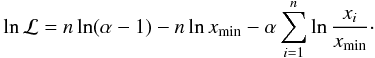 (A.2)Maximum Likelihood Estimations (MLEs) face a special problem when applied to power-laws: the parameter xmin is both a variable of the density function and a lower bound for the function’s domain. As the likelihood function increases monotonically with decreasing domain, the MLE for xmin converges to ∞ or max(xi). For this reason maximization of the likelihood function is only possible for the parameter α with a conditioned xmin. If we set ∂lnℒ /∂α = 0 we obtain an estimator for the scaling parameter α:
  (A.3)Equation (A.3)is known as the Hill estimator (Hill et al. 1975).
Common approaches for getting an estimator for xmin used visual inspection of log-log plots of the distribution function or so called Hill plots (α vs. the conditioned xmin). CSN07 introduced an algorithm where the best estimator for xmin is obtained by applying Kolmogorov-Smirnov (KS) statistics. For every value xi in the order statistics (the set of the ordered values of the sample) one assumes this value is xmin and calculates the corresponding Hill estimator α(xmin). One also calculates the KS-statistics for this value, which is defined as the maximum difference between the empirical survival function  (A.4)(where I is the indicator function, that takes the value 1 if the argument is true and 0 otherwise) and the theoretical survival (see Eq. (3)) function with that xmin and α. As best fit one accepts the estimators xmin and α(xmin) which minimize the KS-statistics.
For the error estimation of the parameters CSN07 suggest the following bootstrapping technique: first, about 1000 samples each of length n are created by bootstrapping with replacement. For each sample, a power-law fit is performed. The errors for xmin and α(xmin) are then given by taking the standard deviation of the 1000 bootstrapped values for xmin and α(xmin).
A goodness of fit parameter is derived by a modified bootstrapping technique. About 2500 surrogate samples of length n are created. Let ntail be the length of the power-law tail with xi ≥ xmin. Then each value of a surrogate sample is generated as follows: with a probability of ntail/n a random variable from the fitted power-law with xmin and α is drawn, with a probability of 1 − ntail/n a value from the original data set with x<xmin. For each of the surrogate samples a power-law fit is performed and the KS value is noted. The goodness of fit (p-value) is defined as fraction of surrogate data sample which have larger KS-values than the original data set. If the p-value is below a chosen significance level (e.g., 0.05), the power-law hypothesis is rejected. In this case there are only 5% of the surrogate samples with KS-statistic larger than the one of the “best” fit, meaning that most of the “fake” data fit better the model. In the opposite case, where the p-values are large, the majority of the fake samples have KS-statistics larger than our best fit, so its KS-statistic can be seen as a statistical fluctuation.
Appendix B: Convolution of a pure power-law with a Gaussian distribution
Here we show the influence of uncertainties and noise in the data acquisition on the obtained power-law parameter xmin. We assume an power-law distributed random variable and an error statistics which can be modeled by a Gaussian distribution. Provided that both probabilities are independent the joint probability density is given by the convolution. A schematic representation of this convolution is depicted in Fig. B.1. It can be seen that the apparent lower bound of the power-law, that is the parameter xmin which is obtained by a power-law fitting routine, takes a higher value due to the uncertainty distribution. Nevertheless the power-law index α does not change significantly. A detailed quantitative discussion about power-laws convolved with a Gaussian can be found in Sect. 3.2 of Witzel et al. (2012).
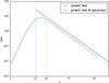 |
Fig. B.1 Schematic example for the convolution of a power-law with a Gaussian distribution and its effect on the apparent xmin. Due to the influence of the Gaussian uncertainty distribution the fitted lower bound x2 takes a higher value than the intrinsic paramter x1. |
All Tables
Comparison of the results for the submm data from parameter estimation approaches.
Comparison of the results (for the radio data) from the CSN07 fitting method (I) to the results from the RKE09 algorithm (II).
All Figures
|
Fig. 1 Data reduction process for the LABOCA campaigns. All maps are zoomed to the innermost 3.5′× 3.5′. Left: a single measurement map of the GC from 2009-05-17T04:19:58. Center: model of the extended submm emission from the GC: co-added maps with subtracted point source at the position of Sgr A*. Right: remaining map for the 2009-05-17T04:19:58 map after subtraction of the GC model for the extended emission. The point like source represents the submm emission from Sgr A* itself. |
| In the text | |
|
Fig. 2 Top: all available submm light curves between 2004 and 2014. The plot contains both the LABOCA data (blue circles) and the literature data (green down-pointing triangles: Eckart et al. 2009; cyan left-pointing triangles: Yusef-Zadeh et al. 2006a; magenta right-pointing triangles: Yusef-Zadeh et al. 2008; yellow squares: Yusef-Zadeh et al. 2009; red up-pointing triangles: Trap et al. 2011). Bottom: a concatenated light curve of the submm data. Time gaps greater than 10 min were replaced by gaps of 300 s. |
| In the text | |
|
Fig. 3 Top: all ATCA 100 GHz light curves obtained between 2010 and 2014. The flux density values are averaged over a window of 300 s. Bottom: concatenated light curve of the averaged radio data after background reduction and removal of negative values. Time gaps greater than 10 min were replaced by gaps of 300 s. |
| In the text | |
|
Fig. 4 Histogram of the submm flux density values. The steady quiescent emission leads to the average of ~3 Jy, the high-flux tail up to ~6 Jy is supposedly power-law distributed. |
| In the text | |
|
Fig. 5 PDFs for shifted power-laws (α = 12, xmin = 3.5) with different shifts, solid line without shift, dashed line with positive, dash-dot line with negative shift. The slope only becomes constant for large x. |
| In the text | |
|
Fig. 6 log-log histogram of the submm data. The curvature of the high-flux tail ≳ 3.5 Jy indicates a shifted power-law of the form p(x) ~ (x − s)α. |
| In the text | |
|
Fig. 7 Quiescent emission model A: subtraction of a constant contribution from the data. In this example the steady contribution is the lowest 30th percentile of all data points. |
| In the text | |
|
Fig. 8 Quiescent emission model B: linear detrending, followed by the subtraction of a global constant for the quiescent emission (not depicted in this plot). |
| In the text | |
|
Fig. 9 Quiescent emission model C: subtraction of a variable quiescent emission. In this example for each campaign the 10th percentiles of the campaign’s data is subtracted. |
| In the text | |
|
Fig. 10 Quiescent emission model D: the variable quiescent emission is modeled by a cubic spline. Here the spline fit is applied to the 20th percentile values of each campaign. |
| In the text | |
|
Fig. 11 log-log histogram of the submm flux density with shifted power-law fit (blue line) from the RKE09 algorithm and a pure power-law fit (green line) according to CSN07. The obtained power-law indices for the RKE09 and CSN07 method are α~4 and ~ 12, respectively. |
| In the text | |
|
Fig. 12 Histogram of the 100 GHz flux density values. |
| In the text | |
|
Fig. 13 log-log histogram of the radio flux density with power-law fits. Both the CSN07 (green line) and the RKE09 (blue line) method yield similar fits, the power-law slopes are within uncertainties consistent with α ~ 4. |
| In the text | |
|
Fig. 14 Schematic representation of possible peak contributions to different frequency channels from different temporal spectra of adiabatically expanding flares. |
| In the text | |
|
Fig. B.1 Schematic example for the convolution of a power-law with a Gaussian distribution and its effect on the apparent xmin. Due to the influence of the Gaussian uncertainty distribution the fitted lower bound x2 takes a higher value than the intrinsic paramter x1. |
| In the text | |
Current usage metrics show cumulative count of Article Views (full-text article views including HTML views, PDF and ePub downloads, according to the available data) and Abstracts Views on Vision4Press platform.
Data correspond to usage on the plateform after 2015. The current usage metrics is available 48-96 hours after online publication and is updated daily on week days.
Initial download of the metrics may take a while.