| Issue |
A&A
Volume 601, May 2017
|
|
|---|---|---|
| Article Number | A10 | |
| Number of page(s) | 23 | |
| Section | Stellar atmospheres | |
| DOI | https://doi.org/10.1051/0004-6361/201525886 | |
| Published online | 19 April 2017 | |
A grid of MARCS model atmospheres for late-type stars
II. S stars and their properties⋆,⋆⋆,⋆⋆⋆
1 Institut d’Astronomie et d’Astrophysique, Université Libre de Bruxelles (ULB), CP 226, Boulevard du Triomphe, 1050 Bruxelles, Belgium
e-mail: This email address is being protected from spambots. You need JavaScript enabled to view it.
2 Laboratoire Univers et Particules de Montpellier, Université de Montpellier, CNRS, 34095 Montpellier, France
3 Department of Physics and Astronomy, Division of Astronomy and Space Physics, Uppsala University, Box 515, 751 20 Uppsala, Sweden
4 Niels Bohr Institute, Juliane Maries vej 30, 2100 Copenhagen, Denmark
5 Centre for Star and Planet Formation, Geological Museum, Øster Voldgade 5, 1350 Copenhagen, Denmark
Received: 13 February 2015
Accepted: 23 July 2016
Abstract
S-type stars are late-type giants whose atmospheres are enriched in carbon and s-process elements because of either extrinsic pollution by a binary companion or intrinsic nucleosynthesis and dredge-up on the thermally-pulsing asymptotic giant branch. A grid of MARCS model atmospheres has been computed for S stars, covering the range 2700 ≤ Teff(K) ≤ 4000, 0.50 ≤ C/O ≤ 0.99, 0 ≤ log g ≤ 5, [Fe/H] = 0., −0.5 dex, and [s/Fe] = 0, 1, and 2 dex (where the latter quantity refers to the global overabundance of s-process elements). The MARCS models make use of a new ZrO line list. Synthetic spectra computed from these models are used to derive photometric indices in the Johnson and Geneva systems, as well as TiO and ZrO band strengths. A method is proposed to select the model best matching any given S star, a non-trivial operation since the grid contains more than 3500 models covering a five-dimensional parameter space. The method is based on the comparison between observed and synthetic photometric indices and spectral band strengths, and has been applied on a vast subsample of the Henize sample of S stars. Our results confirm the old claim by Piccirillo (1980, MNRAS, 190, 441) that ZrO bands in warm S stars (Teff>3200 K) are not caused by the C/O ratio being close to unity, as traditionally believed, but rather by some Zr overabundance. The TiO and ZrO band strengths, combined with V−K and J−K photometric indices, are used to select Teff, C/O, [Fe/H] and [s/Fe]. The Geneva U−B1 and B2−V1 indices (or any equivalent) are good at selecting the gravity. The defining spectral features of dwarf S stars are outlined, but none is found among the Henize S stars. More generally, it is found that, at Teff = 3200 K, a change of C/O from 0.5 to 0.99 has a strong impact on V−K (2 mag). Conversely, a range of 2 mag in V−K corresponds to a 200 K shift along the (Teff, V−K) relationship (for a fixed C/O value). Hence, the use of a (Teff, V−K) calibration established for M stars will yield large errors for S stars, so that a specific calibration must be used, as provided in the present paper. Using the atmospheric parameters derived by our method for the sample of Henize S stars, we show that the extrinsic-intrinsic dichotomy among S stars reveals itself very clearly as a bimodal distribution in the effective temperatures. Moreover, the increase of s-process element abundances with increasing C/O ratios and decreasing temperatures is apparent among intrinsic stars, confirming theoretical expectations.
Key words: stars: atmospheres / stars: fundamental parameters / stars: late-type / stars: AGB and post-AGB / stars: abundances / stars: general
Based on observations carried out at the European Southern Observatory (ESO, La Silla, Chile; program 58.E-0942), on the Swiss 70 cm telescope (La Silla, Chile) and on the Mercator telescope (La Palma, Spain).
The MARCS S star model atmospheres will be archived on the MARCS website: http://marcs.astro.uu.se
Full Tables 2 and 3 are only available at the CDS via anonymous ftp to cdsarc.u-strasbg.fr (130.79.128.5) or via http://cdsarc.u-strasbg.fr/viz-bin/qcat?J/A+A/601/A10
© ESO, 2017
1. Introduction
The S class was originally defined by Merrill (1922) to designate a group of intriguing red stars which did not fit well into either class M (cool stars with titanium oxide bands) or classes R and N (carbon stars). Keenan (1954) clarified the situation by accepting as S stars only those exhibiting zirconium oxide bands. The numerous attempts to link phenomenological spectral classification criteria to physical parameters (effective temperature Teff, gravity g, C/O, [Fe/H], [s/Fe]1; Keenan 1954; Keenan & McNeil 1976; Ake 1979; Keenan & Boeshaar 1980) only lead to imprecise results, because low-resolution diagnostics are strongly entangled in terms of Teff, C/O and [s/Fe] variations. This is the reason why models for S-type star atmospheres are virtually non-existent, the only in-depth discussion of their thermal structure and spectra dating back to the pioneering paper of Piccirillo (1980). That paper concluded that the temperature and C/O ratio have a strong influence on the atmospheric structure of S stars, whereas the S-star spectra are moreover impacted by the s-process overabundances. Piccirillo’s investigation was however limited because important molecular opacity sources were not available at the time. In particular, ZrO opacities were lacking and this was a major obstacle in the S star modelling until now. Most subsequent analyses of S stars even more crudely relied on models designed for M-type stars, not allowing for variations in the C/O or [s/Fe] ratios.
Here we present a grid of MARCS model atmospheres using a new ZrO linelist and covering the parameter space of S-type stars. We attempt to provide a calibration of photometric and band-strength indices in terms of Teff, log g, C/O, [Fe/H], and [s/Fe].
Section 2 presents the ingredients of the new MARCS models of S stars, and discusses the specific properties of their thermal and pressure structures as compared to those of M giants. In Sect. 3, photometric and band-strength indices computed from synthetic spectra are compared to those of S stars from the Henize sample. This comparison allows us to assign atmospheric parameters to a sample of 106 S stars, following a method outlined in Sect. 4. These atmospheric parameters are then used to derive the Zr and Fe abundances from high-resolution spectra, and the abundances derived that way are in good agreement with the [s/Fe] and [Fe/H] parameters used to select the model atmosphere and inferred on the basis of photometric indices, and of TiO and ZrO band-strength indices. This comparison thus validates our method.
In Sect. 5, the atmospheric parameters are used for comparing the properties of extrinsic and intrinsic S stars. These two distinct subclasses are defined on the basis of the presence or absence of lines from technetium, an element with no stable isotopes (see Van Eck & Jorissen 1999,and references therein). The intrinsic/extrinsic dichotomy makes it possible to distinguish S stars in an active nucleosynthesis phase on the asymptotic giant branch (AGB) from S stars in binary systems with a white dwarf companion, formerly an AGB star, which polluted its companion (the current S star) with s-process elements, leading to the currently observed fossil overabundances in s-process elements. Dwarf S stars, the dwarf counterparts of extrinsic giant S stars, have never been observed yet, but at the end of Sect. 5 an attempt is made to characterize them spectroscopically.
The important role that bright giants and supergiants play in, for example, population synthesis and integrated light analysis of old “red and dead” objects such as Galactic and extra-galactic globular clusters and nearby dwarf spheroidal galaxies, has been uncovered recently (e.g. Maraston 2011,and references therein). Since stellar population models used in galaxy modelling require the evaluation of the spectral energy distribution, it is important to be able to compute realistic spectra of AGB stars, including S stars, as we describe in the present paper. S and MS stars are indeed known to co-exist with M and C stars along the TP-AGB of external systems (see for instance Lundgren 1988 for the brightest TP-AGB stars in LMC, which are of MS type; or Boyer et al. 2015 and Lloyd Evans 2004 for the largest census of S stars in the Magellanic Clouds).
2. The models
2.1. Ingredients
A very large new grid of MARCS model atmospheres (Gustafsson et al. 1975; Plez et al. 1992; Asplund et al. 1997) is now being completed (see Gustafsson et al. 2003a,b, 2008).
The characteristics of the set of S-star models presented here are the following:
-
2700 K ≤ Teff ≤ 4000 K (step 100 K);
-
0 ≤ log g ≤ 5 (step 1 dex);
-
M = 1 M⊙;
-
C/O ratios from 0.5 to 0.99 (0.50, 0.75, 0.90, 0.92, 0.95, 0.97, 0.99);
-
[Fe/H] = 0.0 and −0.5;
-
[s/Fe] = 0.0, +1.0, and +2.0;
-
[α/ Fe] = −0.4 × [Fe/H];
-
microturbulence χ = 2 km s-1;
-
opacities as complete and accurate as possible. A special effort has been invested in this work to improve the ZrO line list;
-
opacity sampling with >105 wavelength points, covering the spectral region 912 Å–20 μm, which is satisfactory for the total flux integration in the considered effective temperature range;
-
Local thermodynamic equilibrium (LTE), mixing-length theory of convection, and spherical symmetry for log g ≤ 3, otherwise plane-parallel structure.
The basic ingredients in the model calculations were chosen to be consistent with that of the general MARCS grid (Gustafsson et al. 2008). This concerns the metal line opacity data and the basic solar reference abundance scale presented by Grevesse et al. (2007). Only lines of neutral and singly ionized species are considered. The elements Ne, Mg, Si, S, Ar, Ca, and Ti are collectively considered as α elements. The prescription for [α/Fe] was chosen so as to follow the trend observed for galactic disk stars (McWilliam 1997,and references therein). [O/Fe] follows [α/Fe].
Concerning the opacity tables, the MARCS opacity calculation includes the ZrO molecule, as well as neutral and first ionized levels of all stable atoms. Isotopes of elements heavier than Zn were considered to be produced through the rapid and/or slow neutron-capture processes. For atomic numbers 31–38 (Ga-Sr), the s-process fractions were adopted from Käppeler et al. (1989). For higher atomic numbers, we used the corresponding data from Arlandini et al. (1999). Proton-capture isotopes were neglected and an r-process origin was assumed for the remaining fraction of each isotopic abundance. Thus, just above 30 000 metal lines with varying fractions of s-process nuclei were used in the model calculations.
As in Gustafsson et al. (2008), the mixing length parameter α = l/Hp and the two other parameters (y and ν) describing the convective atmosphere have been chosen following Henyey et al. (1965): α = 1.5, y = 0.076 and ν = 8. The use of a local theory of convection inevitably brings in uncertainties (compared to 3D hydrodynamical models), whatever choice of the convection parametrization. The impact on the model structure of changing α is small however (see Gustafsson et al. 1975, 2008).
We have included turbulent pressure ( , with β = 0.5, and vt = vMLT). Magic et al. (2013) have shown that whatever choice is made for β, the turbulent pressure calculated in 3D models cannot be reproduced using the MLT velocity. Also, 3D models show an increasing Pturb in the outer layers (log τ< −2) due to wave activity in the outer atmosphere. This cannot be modelled by MLT. Chiavassa et al. (2011) have shown that the effect of Pturb on the atmospheric structure can be reproduced using 1D models with a reduced gravity, following the recipe given in Gustafsson et al. (2008): a model with a given turbulent velocity can be represented, to a good approximation, by a model with a reduced gravity (geff, their Eq. (9)) and vt = 0 km s-1.
The strong line blending in S-star spectra prevents the microturbulence determination by the standard spectroscopic method; the adopted value is typical for this kind of giants. The ZrO line list was assembled in the same way as the TiO line list of Plez (1998), using data from Afaf (1995), Balfour & Tatum (1973), Davis & Hammer (1988), Hammer & Davis (1979, 1980), Huber & Herzberg (1979), Jonsson (1994), Jonsson et al. (1995), Kaledin et al. (1995), Langhoff & Bauschlicher (1988, 1990), Lindgren (1973), Littleton & Davis (1985), Littleton et al. (1993), Phillips & Davis (1976a,b), Phillips et al. (1979), Simard et al. (1988), Tatum & Balfour (1973). The list contains lines of the electronic transitions B1Π−A1Δ, B1Π−X1Σ+, C1Σ+−X1Σ+, E1Φ−A1Δ, b3Π−a3Δ, d3Φ−a3Δ, e3Π−a3Δ, f3Δ−a3Δ, for v′ and v′′ up to 30 and J up to 200, for 90,91,92,94,96ZrO. The completeness of our ZrO line list is similar to the one of our TiO line list.
Unequal C/O spacing has been adopted in order to regularly sample changes in the thermal structure as well as in the resulting optical spectra. Indeed, when C/O approaches unity, major changes occur even for tiny C/O variations; therefore the C/O spacing decreases with increasing C/O.
The solar-metallicity oxygen abundance has been taken equal to log ϵ(O) = 8.66. A total of 3525 converged model atmospheres of S stars (turning into M stars when C/O = 0.5 and [s/Fe] = 0.0) were obtained.
In term of absolute bolometric luminosity, the (squared) grid extends from Mbol=9.4 or 7.7 (for log g = 5, Teff=2700 K or 4000 K) up to Mbol=−4.7 or −3.0 (for log g = 0, Teff=2700 K or 4000 K). The radii range from 0.5 R⊙ to 165 R⊙.
The parameters previously determined in the literature for field galactic S stars, on the basis of medium-to-high-resolution spectra, lie in the following ranges: 3200 K ≤ Teff ≤ 3700 K, −0.07 ≤ log g ≤ 1, −0.85 ≤ [Fe/H] ≤ 0.17 (Harris et al. 1985; Smith & Lambert 1986; Vanture & Wallerstein 2003; Pompéia 2009). Smith & Lambert’s C/O determinations (Smith & Lambert 1986) are all smaller than 0.74. Other authors commonly adopt solar C/O ratios. The [s/Fe] ratios measured so far are always smaller than 2. Our grid covers these ranges and even extends beyond, for example allowing for the existence of yet unobserved but anticipated dwarf S stars (see Sect. 5.2).
As far as the mass is concerned, a value of 1 M⊙ has been adopted. Since extrinsic S stars are evolved barium stars, their mass distribution can be estimated by inverting the mass function derived from the many orbital elements known for barium stars. The inversion was done in Jorissen et al. (1998) and masses of ~ 1.6M⊙ were found for both barium stars and extrinsic S stars.
Concerning intrinsic S stars, both stellar evolution models and abundance determinations provide constraints on the mass. Models predict that their mass should be larger than 1.0–1.5 M⊙ (depending on metallicity), otherwise no third dredge-up occurs (Siess, priv. comm.). From a comparison of s-process element abundances with evolutionary models, the mass of intrinsic S stars has been estimated to lie between 1 and 3 M⊙ (Neyskens et al. 2015). Here we adopted M = 1M⊙; the impact of mass on the model structure is discussed in the next section.
2.2. Thermal and pressure structures
Plots of the evolution of T, Pgas, τ500, and τRoss (where τ500 is the optical depth at 500 nm, and τRoss is the Rosseland optical depth) for models with different C/O ratios (Fig. 1) show that:
-
the Pgas – τ1 μm relation stays basically unchanged when C/O varies(because it is governed mostly by log g);
-
the T – τRoss relation (governed by the energy balance requirement) reaches higher temperatures at the surface for higher C/O ratios;
-
when C/O increases, Pgas at a given T increases.
The latter effects are due to a large decrease of the partial pressures of H2O and TiO, two major opacity contributors, when C/O approaches unity. Conversely, the partial pressure of CO increases at higher C/O values. The blanketing effect of H2O and TiO then decreases dramatically. At a given τ500, τRoss becomes much smaller, and the outer layers of the atmosphere (those with small τRoss) are shifted to much higher pressures. In principle, this decreased blanketing leads to less back-warming – i.e. cooler structures around τ500 = 1, such that less flux is produced in the near IR. This is seen in the upper right panel of Fig. 1 and in Fig. 2 (J band in particular). The diminished TiO and H2O band strengths also lead to different surface temperatures. However, since TiO is mainly heating the upper layers while H2O is mainly cooling them (see discussion in Gustafsson et al. 2008,their Sect. 6.1), the combined effect is complex.
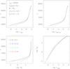 |
Fig. 1 Thermal and gas pressure structures of model atmospheres of S stars with Teff = 3000 K, log g = 0, M = 1 M⊙ and various C/O ratios, as labelled, for a global s-process enrichment [s/Fe] = +1 dex. Pg is expressed in cgs. |
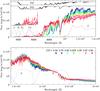 |
Fig. 2 Influence of the C/O ratio on synthetic spectra obtained for the models corresponding to the thermal structures displayed in Fig. 1: Teff = 3000 K, [s/Fe] = 1 dex, log g = 0, M = 1 M⊙, [Fe/H] = 0, and C/O ratios as labelled. The U,B,V,V1,J,H,K bandpasses are plotted in black dashed lines, as well as, in black on the top panel, synthetic spectra of pure TiO and pure ZrO (for the same temperature and C/O = 0.5) to help identifying molecular-band contributors. For the sake of clarity, spectra are also zoomed shortward of 6500 Å. |
As expected, the C/O ratio has a major impact on the structure of the models, whereas the [s/Fe] ratio has a minor importance. The impact of ZrO on the models can be estimated directly from the [s/Fe] impact, since ZrO is the most prominent molecule involving an s-process element. The effect on the model structure is minor, as can be seen from Fig. 3. Despite this minor effect on the thermal structure, ZrO bands have a prominent impact on the spectral appearance, as we discuss in the next section.
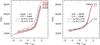 |
Fig. 3 Temperature as a function of the optical depth at 1 μm for S-star model atmospheres. Left panel: for different effective temperatures, as labelled, but a typical gravity (log (g) = 0) and C/O ratio (C/O = 0.899) of S-type stars, the thermal structure shows only minor changes between non-enhanced ([s/Fe] = 0 dex, continuous lines) and enhanced ([s/Fe] = +2 dex, dashed lines) models. Right panel: same as left panel, but for a given effective temperature (Teff = 3600 K) and varying gravities, as labelled. |
The entire grid of S-star models has been computed with a constant mass M = 1 M⊙. The impact on the model atmosphere of a change in the stellar mass (at a constant gravity) has been investigated. As can be seen in Fig. 4, the temperature profiles of 2 M⊙ and 1 M⊙ models as a function of log τ1 μm cannot be distinguished. The relative temperature differences are indeed very tiny (a few percents) as demonstrated by the panel displaying ΔT/T as a function of log τ1 μm.
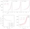 |
Fig. 4 Upper panel: comparison of the effective temperature and atmospheric extension (z/R⋆, where z is the geometrical height in the atmosphere, z = 0 at log (τRoss) = 0), for models with M = 1 M⊙ and 2 M⊙, for three different temperatures, as labelled. The stellar parameters are log g = 0., [Fe/H] = 0, [s/Fe] = 1, C/O = 0.97 for all represented models. Lower panel, left: relative difference in effective temperature of the 2 M⊙ and 1 M⊙ models. Lower panel, right: effective temperature as a function of the optical depth at 1 μm. |
The atmospheric extension z/R⋆ has been investigated by various authors (Plez 1990; Heiter & Eriksson 2006) and better illustrates the differences when changing mass at a given gravity (Fig. 4): 1 M⊙ models are characterized by a larger atmospheric extension than 2 M⊙ models. While this is certainly relevant for interferometric investigations of S-type stars, the results presented in this paper are based on synthetic spectra and colours. The impact on the photometry and on the spectroscopic indices (used here to determine S-star parameters) is illustrated in Figs. 5 and 6. The largest differences are observed for cool (3000 K) models, where 2 M⊙ models are slightly bluer than 1 M⊙ models (Δ(V−K) = 0.1 mag). 1 M⊙ spectra display slightly stronger molecular lines, because in the external layers, at a given τ1 μm, the atmospheric extension z/R⋆ is larger and the gravity is lower, while the temperature remains basically unchanged. Therefore the gas pressure is larger in the external layers of 1 M⊙ models. The increase of absorbers column density in the outer atmospheric layers leads to slightly stronger lines, and slightly redder colours in the lower mass models. This effect is however negligible as seen in Figs. 5 and 6. The choice of a unique mass for the whole S star model grid is well justified.
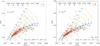 |
Fig. 5 Dereddened (V−K,J−K) colour–colour diagram for Henize S stars (open triangles) and M giants (open circles, from Whitelock et al. 2000) and a few C stars (crosses, from Whitelock et al. 2000), as compared to model colours (grid) of different effective temperatures and C/O ratios, for log g = 0, M = 1 M⊙, [Fe/H] = 0 and for [s/Fe] = +0 dex (left) or [s/Fe] = +1 dex (right). The effective temperature ranges from 4000 to 2700 K, from bottom to top, as labelled in the figure; models with identical effective temperatures are connected by dashed lines. Different C/O ratios from 0.5 to 0.99 are represented by solid lines, the leftmost for C/O = 0.991, next to that C/O = 0.971, etc. The small error bars on the lower right corner of the [s/Fe] = 1 panel (in V−K and in J−K, barely seen) represent the variation of the colours at Teff = 3000 K of 2 M⊙ models with respect to 1 M⊙ models, 2 M⊙ models being slightly bluer (Δ(V−K) = 0.1 mag) than 1 M⊙ models. The arrow marks the reddening vector for AV = 0.6 mag. |
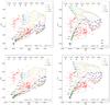 |
Fig. 6 Measured BTiO and BZrO band indices from observed spectra of different stellar types (as labelled) compared to band indices computed from synthetic spectra for the same grid of temperatures (models with identical – as indicated – effective temperatures joined by dashed black lines) and C/O ratios (connected by solid coloured lines, for the same values as those displayed in Fig. 5, the largest C/O value corresponding to the most vertical solid line). The four panels correspond to various combinations of metallicity and [s/Fe] ratio, as labelled. Field stars (radial velocity standards and flux calibrators without molecular bands) are clumping around (BTiO, BZrO) = (0, 0), as expected. The small error bars on the lower right corner of the [Fe/H] = 0, [s/Fe] = 1 panel represent the largest variations (computed at 3000 K, 3400 K and 3800 K) of the indices of 2 M⊙ models with respect to 1 M⊙ models, 1 M⊙ models having slightly stronger lines (and larger indices) than 2 M⊙ models. |
2.3. Synthetic spectra
Synthetic spectra of a series of models with different C/O ratios demonstrate the decrease of the TiO and H2O band strengths with increasing C/O (Fig. 2). This results in higher flux levels in the optical and at longer IR wavelengths. At C/O = 0.99, the spectral energy distribution appears flatter between the optical and the H-opacity minimum at 1.6 μm, with the flux peak being displaced towards the H band in the cooler models. This is the result of a decrease of the continuum level around 1 μm, and an increase of the CN line strengths. The K band is little affected by C/O and [s/Fe] variations, the CO lines being saturated and the C abundance varying by not more than a factor of 2. Figure 5 clearly demonstrates that the C/O ratio has a considerable impact on the (V−K,J−K) colour indices for all S stars with C/O ≥0.90 and Teff≤3200 K.
Finally, larger s-element abundances induce large changes in the optical spectrum, through stronger ZrO bands. This is apparent in Fig. 7, which reveals that the synthetic spectrum corresponding to Teff = 3000 K, C/O = 0.99 and [s/Fe] = 1 dex is quite depressed shortwards of 650 nm, as compared to the corresponding spectrum with solar s-process abundances. S stars with C/O = 0.99, Teff = 3000 K and [s/Fe] = 1 dex thus appear redder by almost 1 mag in the V−K index, as compared to their M-star counterparts with solar s-process abundances (compare left and right panels of Fig. 5). However, since ZrO bands are found mainly in the optical, where the flux is relatively small, the impact on the thermal structure is quite limited (Sect. 2.2 and Fig. 3).
In Sect. 3 we exploit this spectral sensitivity to the C/O ratio and s-element abundances to devise spectroscopic and photometric indices which disentangle Teff from the C/O and [s/Fe] ratios in S stars.
3. Confronting the models to observed colours and spectral-band indices
3.1. The Henize sample of S stars
The Henize sample of S stars2 (205 stars with R ≤ 10.5 and δ ≤ −25°; Henize 1960) is of particular interest, since (i) it includes intrinsic as well as extrinsic S stars (Van Eck & Jorissen 2000b); and (ii) a large observational material has been collected for this sample (Van Eck & Jorissen 2000a). Available data include (i) Geneva UBV photometry; (ii) SAAO JHKL photometry; and (iii) low-resolution spectra (Δλ = 3 Å) covering the spectral range 440–820 nm, from the Boller & Chivens spectrograph at the ESO/MPI 2.2-m telescope at La Silla (ESO). These spectra were dereddened according to Cardelli et al. (1989). These data are collected in Table 2. Using multivariate classification including technetium information, radial velocity, photometric variability and infrared colour excess, each Henize S star has been assigned to the intrinsic or extrinsic category (Table 4 of Van Eck & Jorissen 2000a).
3.2. Band-strength indices
Band-strength indices B were computed as follows, for synthetic and observed spectra: 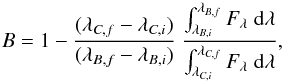 (1)where Fλ is the observed or model flux in the wavelength range (λ, λ + dλ), with the continuum window λC,i−λC,f and band window λB,i−λB,f listed in Table 1.
We note that these band definitions are slightly different from (and supersede) those listed in Table 2 of Van Eck et al. (2000). As discussed in that paper, only those ZrO bands not too strongly contaminated by TiO bands were kept in the analysis. In practice, Pearson’s correlation coefficients between each ZrO band index and the average TiO index were computed for all non-pure S stars. If they were larger than 0.6, the corresponding ZrO band was rejected. The final indices are obtained by a simple average of the individual band indices.
Figure 2 shows that there is a strong ZrO band around 9300 Å. The intensity of this band appears to be very sensitive to the [s/Fe] ratio, and as such, could be a very good probe of s-process overabundances. The Boller & Chivens spectra of S stars mainly used in the present study (Sect. 3.1) did not cover that band, however. It is therefore not listed in Table 1. It is nevertheless used, when available from HERMES spectra, for an independent check of the derived atmospheric parameters (as discussed in Sect. 4.2.3).
3.3. Photometric colours
As already mentioned, Geneva UBVB1B2V1G photometry, obtained on the Swiss Telescope at La Silla (Chile), is available for 179 Henize S stars, with an average of four good-quality photometric measurements (in all filters) per star. Additional JHKL photometry comes from the South African Astrophysical Observatory for 138 stars (Table 2, see also Van Eck & Jorissen 2000a). The interstellar extinction coefficient was computed from the 3D Galactic Extinction Model of Drimmel et al. (2003). The colour excess was then derived as in Van Eck & Jorissen (2000a).
Corresponding photometric colours have been computed on the synthetic spectra, as listed in Table 3. We used the same filters and zero-points as in Bessell et al. (1998a,b) for the Johnson U,B,V,R,I,J,H,K,L filters and computed as well the Geneva U,B,V,B1,B2,V1,G magnitudes. Bessell et al. (1998a,b) used the observed V magnitude of Vega to determine the V zero-point, and the observed colours of Vega and Sirius to determine the zero points of the other filters. The calculated colours for these two stars were all within 0.01 mag of the observations, except for the V−K colour of Vega which deviates by 0.02 mag (see their Table A1).
Johnson and Geneva (G) photometric indices and band indices measured on the observed Henize S stars (full table available at the CDS).
Johnson and Geneva (G) photometric indices and band indices computed on the grid of synthetic spectra of S stars (full table available at the CDS).
3.4. Comparison between models and observations
From these data, the (V−K,J−K) colour–colour diagram has been constructed (Fig. 5). Similarly, BTiO and BZrO band-strength indices have been computed from the low-resolution spectra, and plotted in Fig. 6. Figures 5 and 6 display as well the synthetic indices, and their comparison with the observed values makes it possible to estimate the atmospheric parameters of S stars, namely Teff, C/O, [Fe/H] and [s/Fe], since:
-
The (V−K,J−K) colour–colour diagram disentangles Teff and C/O.
-
The (BTiO, BZrO) diagram disentangles Teff, C/O and [s/Fe].
Figure 5 includes not only S stars, but also M and C stars (Whitelock et al. 2000). We remind that M stars refer to objects with a roughly solar C/O ratio, whereas C stars have C/O >1. As already noted by Piccirillo (1980) and as we shall confirm in this section, S stars have C/O ratios intermediate between those of M and C stars. SC and CS stars, also called D-line stars (Keenan & Boeshaar 1980,and references therein) are rarer and form a continuous sequence between S and C-type stars. Computations of molecular equilibrium (Scalo & Ross 1976) indicate they have C/O = 1 to within about 1%. They are observationally characterized by strong sodium D lines (more generally, many atomic lines are prominent in their spectra), because the spectrum depression by TiO and ZrO molecular bands decreases when C/O reaches unity. SC stars still show weak ZrO bands, while CS stars already show C2 bands.
As expected, the (V−K) and (J−K) indices vary continuously when passing from M stars to C stars through S stars (Fig. 5). The synthetic indices for the models with [s/Fe] = +1 dex and [Fe/H] = 0 cover the region occupied by the Henize S stars. This agreement constitutes an indirect confirmation that the underlying physics and ingredients of the models are globally correct.
The (V−K,J−K) colour–colour diagram (Fig. 5) reveals that, for a given V−K, the range in Teff covered by models of different C/O ratios is about 200 K. Therefore, the application to S stars (C/O >0.5) of the usual M-star (C/O ~0.5) temperature scale based on the V−K index (as done in the past when specific S-star models were unavailable) leads to errors on Teff of up to 200 K. It must be stressed that the photometric sequence becomes quite tight above 3600 K (because of the disappearance of molecular bands affecting the V and J filters, see Fig. 2) and even there, the synthetic photometric indices of the log g = 0, [Fe/H] = 0 and [s/Fe] = 1 grid match the region occupied by the bulk of S and M stars.
Stellar parameters of Henize stars.
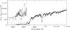 |
Fig. 7 Influence of [s/Fe] on synthetic spectra obtained for the models corresponding to the thermal structures displayed in Fig. 1: Teff = 3000 K, log g = 0, M = 1 M⊙, [Fe/H] = 0, C/O = 0.99 and [s/Fe] = 0 dex (thin dotted line) or [s/Fe] = +1 dex (thick solid line). |
In Fig. 5 there is a number of stars falling below the model grids at (V−K,J−K) ~ (4...8,1). In fact, these objects are well reproduced by the log g = 1 or log g = 2 grid, with [s/Fe] = +0, +1 or +2, as may be judged by the model properties listed in Table 4. Some M stars (green circles) as well as extrinsic S stars (Hen 5, 35, 83) and intrinsic stars (Hen 15, 45, 47, 122, 127, 148, 178, 196) are present in this region. Whereas M and extrinsic S stars can well be less evolved objects, still on the RGB and with higher gravities than thermally-pulsing AGB (TPAGB) stars, the reason why intrinsic S stars are encountered is less obvious, and might be related to the non-simultaneous V and JHK photometry. Incidentally, it may be expected that chemical parameters ([s/Fe] and C/O) for stars with Teff>3700 K will be more difficult to derive, because the photometric sequence becomes totally insensitive to [s/Fe] and C/O. There, high-resolution spectra are needed. However, our S-star sample contains only 3 stars with Teff>3700 K. Therefore the method presented in this paper to derive the model-atmosphere parameters of S stars seems to be valid for the present sample of S stars and, given its representativity, the method should be equally valid for the vast majority of S stars.
As seen in Fig. 6, the TiO and ZrO band strengths in S stars are reasonably well reproduced as well. Again, the synthetic BTiO and BZrO indices indeed tend to (0,0) at high temperatures, as expected for warm stars lacking molecular bands. Models with C/O = 0.5 and [s/Fe] = 0 dex correctly match the TiO (and ZrO) band strengths of M giants, as expected. In particular, as temperature decreases, ZrO bands appear even in M stars. In those cool stars, there is a strong positive correlation between the ZrO band strength and the C/O ratio: even in the absence of any s-process overabundance, strong ZrO bands appear in cool stars with C/O ratios close to unity. This was already shown by former studies based on molecular equilibrium calculations (Scalo & Ross 1976; Piccirillo 1980), and constitutes the foundation for the traditional claim that the M-S-C sequence is one of increasing C/O ratio along the AGB. It must be stressed, however, that this statement does not hold true for the warmer S stars. Figure 6 clearly shows that for Teff≳3400 K, no strong ZrO bands develop in the absence of s-process overabundances even though the C/O ratio approaches unity. For those warm S stars, an s-process overabundance is thus an essential requirement for the development of ZrO bands. Here again, synthetic band indices match well the region populated by S stars. The [Fe/H] = 0, [s/Fe] = 1 dex grid matches especially well the left boundary of the region occupied by S stars, corresponding to C/O = 0.99. Thus, Fig. 6 demonstrates that most S/SC stars have 0.5< [s/Fe] ≤1.
S stars with distinctive LaO molecular bands.
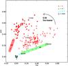 |
Fig. 8 Same as Fig. 6; stars displaying noticeable LaO bands are plotted as filled triangles. Most of them are pure S stars or SC stars. The location of M (C/O ~0.5), S (0.5< C/O <1) and SC stars (C/O ~1) is indicated, as well as some typical effective temperatures. The arrow is an approximative indication of the loop described in this diagram by the stars as they evolve on the TPAGB, as explained in Sect. 3.4. |
There is a group of stars with BTiO ~ 0±0.15 and BZrO ≳ 0.3 which is not at all covered by the models, though. These are pure S stars (i.e. without TiO bands), or SC and CS stars (Table 5). All those stars have C/O very close to unity and the synthesis of their spectral properties do require specific ingredients which are beyond the scope of this paper, for example line lists for CS, HCN, C3, C2H and other polyatomic carbon-bearing molecules (Ferrarotti & Gail 2002). For some of them, a satisfactory solution for the parameters could however be found and is listed in Table 5, since our model atmospheres are, to date, the closest available approximation to SC-type atmospheres. As expected, they all have low temperatures (< 3400 K) and C/O ratios close to unity (they fall in our last 4 C/O bins with C/O >0.92, and often in the highest bin with C/O = 0.99). As displayed in Fig. 8, LaO bands are always detected in their spectra, both because of their strong s-process enhancements and of their weak TiO and ZrO bands. The extreme object at (BTiO,BZrO) = (−0.11,0.143) in Fig. 8 is the remarkable star BH Cru, classified as SC 4.5-7/8e by Keenan & Boeshaar (1980).
The (BTiO,BZrO) diagram thus illustrates the transition nature of S stars, which describe a counterclockwise loop in this diagram, starting from the M sequence (as sketched by the M stars in Fig. 6), evolving to larger TiO and ZrO indices (to the upper right corner in Fig. 6) as the star cools on the AGB and as C and Zr are being dredged-up to the surface, and changing again into pure S stars when TiO bands disappear (to the left in Fig. 6), before showing up as SC stars when, in turn, ZrO bands vanish (downward in Figs. 6 and 8).
To conclude this discussion of the (BTiO, BZrO) diagram, it must be remarked that there is a degeneracy between C/O and [s/Fe] at Teff<3200 K. Even S stars with [s/Fe] =1 dex have relatively weak ZrO bands when C/O <0.9, and fall in the same region of the diagram as the stars lacking s-process overabundances. Those weak ZrO bands are due, in fact, to the strength of TiO bands, that considerably depress the continuum and somehow affect, at such low temperatures, the ZrO indices. The way to handle this degeneracy is explained in Sect. 4.
4. Deriving stellar parameters of S stars from low-resolution data
4.1. Best-model selection
A procedure deriving the best atmospheric parameters for a given S star has been developed (and tagged as BMF for “best-model finding procedure” in what follows). It simply identifies the model for which χ2 is minimum, with:  (2)where Bi,model and Bi,obs are the observed and the synthetic indices as defined in Sects. 3.2 and 3.3. More precisely, the BMF procedure uses the following pairs of indices (Bi)/ weights (wi): dereddened Geneva U−B1 (w = 3), B2−V1 (w = 2), V−K (w = 8), J−K (w = 3), H−K (w = 1), BTiO (w = 12), BZrO (w = 8) and BNa (w = 14), as listed in Table 1. The weight attributed to a given index appeared to be critical to ensure consistent results over the whole parameter space. The variance
  was computed over the whole grid for any given index Bi. The quantities
  amount to: 15.23 (for BTiO), 25.37 (for BZrO), 18.68 (for BNa), 0.27 (for V−K), 21.22 (for J−K), 263.15 (for H−K), 12.32 (for U−B1), 12.67 (for B2−V1).
The adopted values ensure a good agreement between:
-
observed and synthetic low-resolution spectra, particularly inthe many regions not covered by the adopted band-strengthindices; two examples are illustrated in Fig. 9;
-
C/O ratios, [s/Fe] and [Fe/H] abundances obtained from low- and high-resolution data (see Sect. 4.2.3).
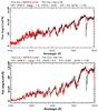 |
Fig. 9 Comparison between the observed low-resolution optical spectrum (thin black line) and the best synthetic spectrum as selected by the BMF procedure (thick red line) for two (intrinsic) S stars of different temperatures: Hen 4-45 (top) and Hen 4-8 (bottom). The atmospheric parameters of the model used to compute the synthetic spectrum are given at the top of each subpanel. Telluric O2 is responsible for the 7600 Å feature. The remaining discrepancies might be caused by telluric H2O (7160 Å), unaccounted LaO bands (e.g. 5580 Å) or remaining inaccuracies in the available molecular linelists. |
This consistency was not at all guaranteed a priori, and provides certainly a strong indication of the validity of the method in general, and of the models in particular.
Section 3.4 explained how Teff and C/O can be disentangled using the V−K and J−K colours, and how BTiO and BZrO disentangle Teff, C/O and [s/Fe]. In turn, gravity is constrained mainly by: (i) for cooler stars, V−K, BTiO and BZrO indices, sensitive to gravity because of the disappearance of strong TiO and ZrO bands in dwarf stars; (ii) for stars hotter than ~ 3400 K, the Geneva colour indices (see Fig. 2 for the bandpasses of the Geneva U, B1, B2 and V1 filters) U−B1 and B2−V1 (or equivalently the Gunn u−v, v−g indices or Strömgren u−v, b−y), strongly gravity-dependent as illustrated in Fig. 10 (where the dotted lines represent the hottest models).
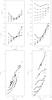 |
Fig. 10 Geneva colours computed from synthetic spectra of S stars with C/O = 0.90 (left panels) and C/O = 0.99 (right panels). Models are computed for [Fe/H] = 0.0 and [s/Fe] = 1 dex. Top panel: U−B1 and B2−V1 as a function of surface gravity. Model temperatures range from 3000 K (thick continuous line) to 4000 K (thin dotted lines), by steps of 200 K (corresponding to the 4 intermediate continuous lines). Bottom panel: (U−B1, B2−V1) plane for different gravities ranging from log g = 0 (thick continuous line) to log g = 5 (thin dotted line), as labeled, and for temperatures ranging from 4000 K (smaller indices) to 2700 K. These figures illustrate the sensitivity of these colours to gravity, especially for low-gravity (log g < 3) warm (Teff≥3400 K) stars. |
Conversely, gravity cannot be safely constrained when the U−B1 and B2−V1 colours are missing. Among S stars, a number of Miras have variable, blue U−B1 colours, leading to spuriously high gravities. They were discarded in the present study (see discussion in Sect. 5.2).
4.2. Consistency checks
4.2.1. Accuracy test
Results of the accuracy test.
To estimate the uncertainty on the stellar parameters determined through the BMF procedure, a blind test was performed. We computed three test model atmospheres, representative of typical S stars, but with parameters (Teff, log g, C/O, [s/Fe]) falling in-between grid points. The resulting synthetic spectra were then treated as real observations: their photometric colours and band-strength indices were ingested in the BMF procedure, resulting in the parameter set presented in Table 6. Due to the grid discretization, the model with Teff, log g, C/O, and [s/Fe] best matching the test model parameters is not always the first one selected by the code, but always lies within the first three selected models. Quantitatively, if  represents the minimum χ2 value obtained by the BMF procedure, the best-matching model is always found in the range
 ![Mathematical equation: \hbox{$[\chi^2_{\rm min}, 1.4~\chi^2_{\rm min}]$}](/articles/aa/full_html/2017/05/aa25886-15/aa25886-15-eq203.png) . The error on the parameters caused by the indices degeneracy and the grid discretization has thus been computed as the range covered by all parameters of all models with χ2 falling in the range . These parameter ranges are listed in Table 4. Below we further discuss the sensitivity of the χ2 when varying the parameters one by one, and how it impacts the sensitivity of the BMF procedure.
. The error on the parameters caused by the indices degeneracy and the grid discretization has thus been computed as the range covered by all parameters of all models with χ2 falling in the range . These parameter ranges are listed in Table 4. Below we further discuss the sensitivity of the χ2 when varying the parameters one by one, and how it impacts the sensitivity of the BMF procedure.
4.2.2. Degeneracy and sensitivity
Variations of χ2 with the parameters (Teff, log g, [Fe/H], C/O, [s/Fe]), starting from a reference model Teff = 3600 K, log g = 0, [Fe/H] = 0, C/O = 0.925, [s/Fe] = +1 dex.
Tables 7 and 8 allow to get more insight on the sensitivity of χ2 to variations of the parameters (Teff, log g, [Fe/H], C/O, [s/Fe]). Representative models have been adopted as reference points. In Table 7 the parameters are Teff = 3600 K, log g = 0, [Fe/H] = 0, C/O = 0.925, [s/Fe] = +1 dex. The upper part of the table shows that the models with the smallest χ2 (and particularly those with 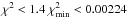 ) have parameters very similar to those of the reference model, which means that the inevitable degeneracy will not drag the solution to very distant loci in the parameter space. The lower parts of Table 7, illustrating the χ2 variations when one parameter is varied at a time, show that the sensitivity is excellent for [s/Fe] (since the χ2 increases dramatically when one departs from the reference model), while it is moderate for Teff, log g and [Fe/H]. The sensitivity to C/O is not optimal: the 5 closest models have similar parameters but differing C/O. This is especially true for the quite warm (Teff = 3600 K) reference model adopted in Table 7, but is less of an issue for cooler models.
From Table 8 computed with a Teff = 3000 K reference model, we see from the ranks that the model selection is very discriminative with respect to [s/Fe], as well as towards large C/O ratios. A lower sensitivity is achieved with respect to Teff, log g, [Fe/H] and small C/O ratios.
Finally, the selected model would in any case be chosen with a  , corresponding in Table 7 to rank 0−1 models, and in Table 8 to rank 0–3 models. Within these ranges, the variation in the parameters is limited, and so is the degeneracy.
4.2.3. Confrontation with high-resolution abundances
As a further check of the BMF procedure, we will in the present section derive the [Fe/H], [s/Fe] abundances and C/O ratio from high-resolution spectra, so as to check the internal consistency of the whole procedure. To this end, high-resolution spectra of all Henize S stars visible from La Palma were obtained with the HERMES spectrograph (Raskin et al. 2011) installed on the 1.2 m Mercator telescope. The spectra were reduced with the standard HERMES pipeline. Our sample is restricted to 6 stars after imposing the availability of Geneva photometry, and after excluding Hen 4-121, a symbiotic S star (Van Eck & Jorissen 2002), and Mira S stars (because their variability does not guarantee that the atmospheric parameters derived from photometric and low-resolution spectral data obtained long ago may be applied to the more recent high-resolution spectra; Sect. 4.3.2). Fortunately enough, these 6 stars happen to cover a fair range in temperatures and C/O ratios.
These high-resolution spectra were then processed in two independent ways:
-
1.
The HERMES spectra (resolution R ~ 86 000) were degraded to the Boller & Chivens resolution (Δλ ~ 3 Å; see Sect. 3.1); from these low-resolution spectra, band-strength indices were computed and the BMF procedure was used to derive the atmospheric parameters C/O, [Fe/H] and [s/Fe] (Cols. 2–6 of Table 9).
-
2.
Spectral synthesis was performed around 23 Fe and 14 Zr lines (using the atmospheric model parameters obtained from step 1), and abundances derived from the comparison with the high-resolution HERMES spectra. The C/O ratio was constrained using CH, CN and C2 bands as well as TiO bands, the strength of which is also sensitive to the C/O ratio. Oxygen lines appeared too blended to be used to derive the oxygen abundance, so that an α/Fe-scaled O abundance was assumed. The corresponding abundances are listed in Cols. 7–9 of Table 9.
Stellar parameters and abundances for the 6 (non-Mira, non-symbiotic) Henize S stars with HERMES high-resolution spectra available.
Table 9 thus compares the abundances derived from the high-resolution spectra to the abundances characterizing the model atmosphere selected by the BMF procedure applied on the low-resolution data. It must be emphasized that the [s/Fe] value derived from the low-resolution spectra relies on the ZrO-band strengths, and is thus independent of the [Zr/Fe] value derived at high resolution from atomic Zr I lines.
As seen on Table 9, the agreement between the two sets of ([Fe/H], [s/Fe], C/O) abundances may be considered as satisfactory.
Even metallicity has been determined quite precisely from the low-resolution indices alone, thanks to the sensitivity of the TiO index on metallicity. The accuracy of the chemical abundances associated to the model atmosphere selected by the BMF procedure gives further (indirect) confidence in the temperature and gravity determinations.
4.3. Uncertainties
4.3.1. De-reddening
As illustrated in Fig. 5, the reddening vector moves the star almost exactly along the temperature sequence: around Teff = 4000 K, an error of 0.1 mag on AV translates into an error of about 30 K on Teff, which reduces to about 20 K around 3200 K. The somewhat uncertain de-reddening is therefore a non-negligible source of uncertainty in the process of deriving the atmospheric parameters outlined in Sect. 4; even worse, in evolved S stars, reddening can also be intrinsic due to a surrounding circumstellar dust shell (Smolders et al. 2012). However, circumstellar reddening is most important in S stars with large mass-loss rates, which are usually strongly variable, but we have restricted our analysis to the least variable stars (σV(ASAS) < 0.5 mag), so these effects should be limited.
More quantitatively, the extinction at a given wavelength λ is related to the monochromatic optical depth with:  (3)where unredenned quantities are indicated with the 0 suffix. An upper limit on τλ can be placed from the [25] − [12] IRAS colour index of Henize S stars. Figure 11 shows that [25] − [12] < −0.15, whereas [25] − [12] = −0.56 would correspond to the absence of dust. The corresponding optical depth can be estimated from Fig. 6 of Ivezic & Elitzur (1995), showing that for oxygen-rich dust, τF< 0.1, where τF is the flux-averaged optical depth (their Eq. (4)). To convert τF to τK, we use Table 1 of Ivezic & Elitzur (1995), where it can be seen that, for optically-thin oxygen-rich stars, τK ≈ 0.5 τF. For the most dusty Henize S stars we can thus write AK ≈ τK ≈ 0.05 mag. If the grain opacity varies approximately as λ-1, then AV ≈ τV ≈ 2.2/0.5 τK ≈ 0.22. Thence we derive the reddening correction E(V−K) = AV−AK = 0.17 mag for the most dusty S stars in our sample. The effect of a dust shell around S stars of our sample (selected to avoid strongly variable stars) is thus relatively moderate but could, in principle, be taken into account as explained above.
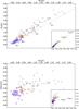 |
Fig. 11 (K− [12] ,K− [25]) (top) and (K− [12] , [25] − [12]) (bottom) colour–colour diagram of Henize S stars. Extrinsic S stars are represented with squares, intrinsic S stars with triangles, and S stars for which no assignment is available (Van Eck & Jorissen 2000a) with circles. The K magnitude is from 2MASS. Only the good-quality (flag = 3) IRAS fluxes have been used. The insets show a wider scale, where 2 outliers (Hen 4-155 and Hen 4-171) are included. The dashed line on the upper panel represents blackbody colours, with arrows corresponding to temperatures ranging between 4000 and 1500 K, as labelled. |
4.3.2. Photometric and spectroscopic variability
Besides the de-reddening process, another source of uncertainty in the derived atmospheric parameters is the non-simultaneity of photometric and spectroscopic data, especially for the most variable stars. In order to estimate the impact of spectroscopic variability, spectroscopic indices have been computed on non-simultaneous data of four S stars for which both Boller & Chivens and HERMES spectra were available. The resolution of HERMES spectra has been degraded to match the lower resolution of Boller & Chivens spectra. The four analyzed stars cover well the parameter range of S stars, with a typical extrinsic star (Hen 4-147), a typical intrinsic semi-regular S star (Hen 4-134) and an intrinsic Mira star (Hen 4-125). The atypical, symbiotic, extrinsic S star Hen 4-121 (Van Eck & Jorissen 2002) has also been included.
Table 10 shows the impact of the spectroscopic variability on the TiO, ZrO and Na indices, while the consequences on the derived stellar parameters are presented in Table 11. For typical extrinsic or even intrinsic S stars (Hen 4-147 and Hen 4-134), the atmospheric parameters are obviously not affected by the extremely small spectroscopic variability. However, for variable stars like symbiotic or Mira stars, the parameter variation can be as large as 200 K in effective temperature; gravity, C/O and [s/Fe] are also affected. This is the reason why the two symbiotic-star parameters should be considered as uncertain (they are flagged as such in Table 4) and the parameters of strongly variable stars (standard deviation σ(VASAS) ≥ 0.5 mag) were not considered reliable enough to be listed in Table 4, and were simply discarded from the present study.
Finally, Table 12 illustrates the impact of the (V−K)photometric variability on the derived parameters. The parameters have been derived for the same four stars, but changing their V magnitude according to their ASAS variability (V ± σASAS(V)). As expected, the large photometric variability of intrinsic S stars impacts their atmospheric structure (typically 100 K in effective temperature, one grid step in C/O). The situation is more favourable for extrinsic stars: despite the small separation between hotter S-star models in the (V−K,J−K) colour–colour diagram, the photometric variability of a typical extrinsic star like Hen 4-147 is not sufficient to affect its atmospheric parameters.
Given these uncertainties, only stars with a standard variation on the ASAS photometry σASAS< 0.5 mag are listed in Table 4 and considered for the following discussion. The only exceptions are the two symbiotic stars, kept despite their blue variable colours, but their uncertain gravity determination is flagged as such in Table 4. The stellar parameters derived for S stars from the Henize sample are listed in Table 4.
Time variability of the spectroscopic indices.
Impact of spectroscopic variability on the stellar parameters.
Influence of photometric (V−K) variability on the stellar parameters.
5. Discussion
5.1. Intrinsic versus extrinsic S stars
The atmospheric parameters derived in Sect. 4 for a large number of intrinsic and extrinsic S stars make it possible to explore their properties, thus pursuing on a more quantitative basis the comparison between the two categories of S stars initiated by Van Eck & Jorissen (2000b). We use the assignment of an S star to either the intrinsic or extrinsic class as derived by Van Eck & Jorissen (2000a).
5.1.1. IRAS photometry
Although not used by the BMF procedure, the IRAS colours of the Henize S stars were investigated, following Van Eck & Jorissen (2000b). K− [12] and K− [25] were colour-corrected according to the IRAS catalogue Explanatory Supplement. Figure 11 illustrates the discriminating power of K− [12], K− [25], and [25] − [12] colours in the framework of the intrinsic/extrinsic dichotomy: extrinsic S stars all have K− [12] < 0.5 and K− [25] < 0.6. Extrinsic S stars also have a negligible V-magnitude variability, when compared to intrinsic S stars.
The two outlier objects with much larger colour excesses (see the insets in Fig. 11) seem to be evolved, highly variable stars: Hen 4-155 (=GN Lup) is a Mira located in the SC star region with (BTiO, BZrO) = (0.01, 0.60) and is indeed classified as S3,8C by Stephenson (1984). Hen 4-171 = C* 2381 was classified as a C star by Stephenson (1984) “on the basis of Wray’s classification. A red Tololo plate shows a late M star with probable weak ZrO”. It shows a large photometric variability (>1.3 mag) and is classified as a possible Mira (M:) in Samus et al. (2004).
5.1.2. Effective temperatures, C/O, [Fe/H], and [s/Fe]
Figure 12 compares the distribution of effective temperatures among intrinsic and extrinsic S stars for all the stars listed in Table 4. There is a clear difference between the two classes, intrinsic S stars being systematically cooler than extrinsic S stars.
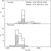 |
Fig. 12 Comparison of the effective temperature distribution of intrinsic (upper panel) and extrinsic (lower panel) S stars collected from Table 4. The dashed line indicates the subset of stars falling in the metallicity bin (−0.75 < [Fe/H] ≤ −0.25), while the shaded histogram concerns stars within the −0.25 < [Fe/H] ≤ 0.25 solar metallicity bin. |
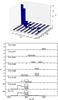 |
Fig. 13 Upper panel: comparison of the effective-temperature distribution of S stars collected from Table 4. Lower panel: same comparison, separating intrinsic (shaded histogram) from extrinsic (dashed histogram) S stars. The total histogram (thick solid line) collects all the stars. |
More quantitatively, 38 out of 109 (extrinsic and intrinsic) S stars have Teff<3350 K, or a fraction of 35%. If the two stellar samples (extrinsic and intrinsic) were drawn from the same parent population, then, when considering solely the sample of 40 extrinsic S stars (of all temperatures), this fraction implies that 13.94 ± 2.40 of them should have Teff<3350 K (the uncertainty on that value is estimated from the hypergeometric distribution, with N = 109, N1 = 40, and p = X/N = 38/109 = 0.35). In the observed sample, zero extrinsic S stars with Teff<3350 K are found, proving that extrinsic and intrinsic S stars have statistically different temperature distributions.
The 7 uppermost panels of Fig. 13 illustrate the effective-temperature distribution split in bins of increasing C/O. This figure is interesting in several respects.
Firstly, there is a trend of decreasing effective temperature when C/O increases.
Again, a simple statistical test can be used to prove the significance of this correlation: let us split the sample in 4 populations with Teff≥ or < 3400 K and C/O> or ≤ 0.9. 8 out of 33 stars have C/O >0.9, or a fraction of 24%. Since 24 stars (all C/O ratio considered) have Teff≥3400 K, then, if there were no correlation between Teff and C/O, one should expect 8/33 × 24 = 5.8 ± 1.1 stars with Teff≥3400 K and C/O >0.9. Here again, the uncertainty is estimated from the hypergeometric distribution, with N = 33, N1 = 24, and p = X/N = 8/33 = 0.24. In the observed sample, only 1 star is found with Teff≥3400 K and C/O >0.9. Therefore, there is a statistically significant (Teff, C/O) correlation among intrinsic S stars (with a significance level better than 3σ).
This trend holds only for intrinsic stars: indeed, when ascending the TP-AGB, such stars are expected to cool down and to exhibit increasing amounts of carbon at their surface as a result of the successive third dredge-up episodes. Extrinsic stars, on the contrary, do show a more limited range of effective temperatures and C/O ratios (3400 K ≤Teff≤ 3800 K, 0.50 ≤ C/O ≤0.75) without any trend, because their C/O ratio is not linked to their present evolutionary stage (and Teff), but instead to a former mass-transfer episode.
The fact that no extrinsic stars are observed with temperatures lower than 3400 K probably reflects the fact that they all turn into intrinsic S stars by the time they reach such low temperatures (i.e. they experience third dredge-up events on the TP-AGB). This result puts a new and strong constraint on the mass of extrinsic S stars. Indeed, a 4 M⊙ star experiences its first third dredge-up at 3713 K (Siess, priv. comm.), whereas this value decreases to 3456 K and 3110 K for 3 and 2 M⊙ stars, respectively (at similar luminosities of roughly 3000 L⊙). We may therefore conclude that the extrinsic S stars of the present sample have masses smaller than 3 M⊙, a result consistent with the average mass of extrinsic S stars, 1.6 or 2.0 M⊙, depending on the adopted white-dwarf mass, a derived by Jorissen et al. (1998) from the cumulative frequency distribution of their orbital mass functions.
Incidentally, the maximum temperature encountered for an extrinsic S star in the present sample is around 3900 K; at higher temperatures, ZrO is sufficiently dissociated so that the star would be classified as barium star and not selected by Henize from his inspection of ZrO bands on low-resolution spectra. A prototypical border case is HD 121447 (not a Henize star), sometimes classified as a barium star and sometimes as an S star (K7III Ba5 or S0; Keenan 1950; Ake 1979; see also Merle et al. 2016 for a recent analysis).
Secondly, the lower C/O ratios derived in extrinsic stars, as compared to the ones measured in intrinsic stars, are the likely result of the dilution in the extrinsic-star atmosphere of the carbon formerly brought from the AGB companion by the mass-transfer episode.
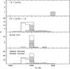 |
Fig. 14 Comparison of the Teff distribution of S stars collected from Table 4, for different s-process enrichment ([s/Fe]) bins. The shaded and dashed histograms correspond to intrinsic and extrinsic stars, respectively, as in Fig. 13. |
Figure 14 illustrates the evolution of the s-process enrichment with effective temperature. The s-process enrichment, [s/Fe], is derived from our BMF procedure, using as main s-process tracer the ZrO molecular-band strength, as described in Sect. 2. The comparison of these values with those derived from a spectroscopic analysis of high-resolution data (Sect. 4.2.3) has shown that the [s/Fe] assignments from low-resolution spectra are accurate to ± 0.4 dex (Table 9). We emphasize that the [s/Fe] value mentioned in Table 4 should rather be considered as [s/Fe] bins with a finite width (namely, [s/Fe] = 0, 1, 2 in fact means [s/Fe] belongs, respectively, to the [−0.5–0.5], [0.5–1.5] and [1.5–2.5] abundance bins).
As for the C/O ratio described earlier, and for the same reason, the largest s-process enrichments ([s/Fe] ~2 dex) occur only in the coolest intrinsic S star (Hen 4-130, Teff = 3000 K, C/O = 0.99).
This is well in line with the loose trend between [Zr/Ti] and Teff observed by Vanture & Wallerstein (2002,their Fig. 3), and naturally results from the fact that cooler stars on the AGB have suffered more thermal pulses and third dredge-ups bringing s-process elements into the envelope. There should not be any such correlation among extrinsic S stars, and indeed, most of the extrinsic S stars fall in the bin [s/Fe] ~1 dex. Neither do Vanture & Wallerstein (2002) find such a correlation for extrinsic S stars. It must be noted though that extrinsic stars being warmer than intrinsic stars (Fig. 13), the sensitivity of both the photometric and spectroscopic indices to [s/Fe] and C/O is much reduced (Figs. 5 and 6), and any trend between the latter two quantities possibly present among extrinsic S stars would be difficult to detect.
Finally, quite a number of S stars belong to the [s/Fe] ~0 dex bin (indicated as [s/Fe] <0.5 dex in Fig. 14). Some of these may simply be modestly s-process enhanced, especially when their C/O ratio is only 0.5, thus typical of M giants. As previously mentioned, all stars with [s/Fe] <0.5 are expected to fall in the [s/Fe] ~0 dex bin.
Such cases are Hen 4-3 (no Tc), Hen 4-6 (no Tc), Hen 4-16 (Tc-rich), Hen 4-20 (Tc-rich), Hen 4-37 (Tc-rich), Hen 4-67 (Tc?), Hen 4-95 (Tc-rich), Hen 4-104 (Tc-rich) and Hen 4-143 (no Tc). At least for the no-Tc cases, they are reminiscent of the so-called Stephenson M stars first encountered by Smith & Lambert (1990), which are stars with no heavy-element overabundances despite being listed in Stephenson’s catalogue of S stars. It should be noted, though, that a high-resolution spectroscopic analysis is needed before any extrinsic star in the above list may be definitely flagged as being a Stephenson M star.
When the nucleosynthesis intrinsic to S stars on the TP-AGB has pushed [s/Fe] to 2 dex, C/O has increased concomittantly (an observation which we ascribe to the fact that both s-elements and carbon are produced in thermal pulses). Therefore, only C/O ratios larger than 0.9 are found when [s/Fe] = 2 dex (Fig. 15).
At intermediate [s/Fe] values (~1 dex), all values of C/O are possible, including those more typical of M stars (C/O ~0.5). Here again, the C/O bin width should be taken into account.
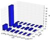 |
Fig. 15 [s/Fe] versus C/O histogram for S stars. |
5.2. Dwarf S stars
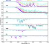 |
Fig. 16 Impact of gravity on the blue-violet synthetic spectra of S stars, as judged from the intensity of the CN, CH, MgH, SiH, CaH, TiO, and ZrO bands. The parameters of the adopted MARCS model atmosphere are Teff = 3000 K, C/O = 0.75, [Fe/H] = 0. dex and [s/Fe] = +1. dex. |
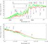 |
Fig. 17 Comparison between synthetic spectra of a giant S star (thin red line) and a dwarf S star (thick green line). Both stars have Teff = 3500 K, C/O = 0.75, [s/Fe] = 1, [Fe/H] = 0, they only differ by their log g value (log g = 0 and log g = 4). Some spectral features are identified (Turnshek et al. 1985; Kirkpatrick et al. 1999). |
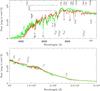 |
Fig. 18 An example of a synthetic low-resolution spectrum of a dwarf S star (thick green line), with Teff = 3800 K, log g = 4, C/O = 0.75, [s/Fe] = 1, as compared with that of an M star of similar Teff, but with log g = 0, C/O = 0.5 and [s/Fe] = 0 (thin red line). |
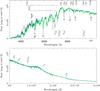 |
Fig. 19 Comparison between dwarf S (thick green line) and dwarf M (thin blue line) synthetic spectra. Both stars have Teff = 3800 K and log g= 4 dex, but C/O = 0.5 (resp., 0.75) and [s/Fe] = 0 (resp., 1) for the M (resp., S) star. |
Our grid of S-star models covers the gravity range from log g = 5 to 0, thus allowing us, in principle, to uncover dwarf S stars, should they exist. Indeed, in the same way that dwarf barium stars (resp., CH dwarfs and carbon-enhanced metal-poor dwarfs) are the high-gravity counterparts of giant barium stars (resp., CH giants and carbon-enhanced metal-poor giants), there is no obvious reason why the coolest s-process enriched dwarfs (too cool to appear as barium dwarfs) should not appear as (extrinsic) S dwarfs. As shown in Figs. 16–18, the general impact of an increasing gravity is to strongly decrease the intensities of the CN, TiO, and ZrO bands, to moderately decrease the intensity of CH, but to increase that of MgH and CaH, while SiH stays almost unaltered.
Several molecular line lists (including LaO, TiS, ZrS, CaOH) are still missing to compute a reliable S-dwarf spectrum. In future works devoted to dwarf S stars, it might be useful to consider whether molecular databases for very late-type stellar atmospheres (e.g. Sharp & Burrows 2007; Tennyson & Yurchenko 2012) could be useful to refine the modelling of such – yet hypothetical – objects.
Nevertheless, a first attempt with the linelists available in the framework of the present model grid is displayed here (Figs. 16−18) in order to identify distinctive features of dwarf S spectra.
Dwarf S stars should be recognizable, like M dwarfs, by strong hydride bands (CaH, MgH, CrH and FeH). Concerning FeH, mainly the 9896 Å band should be useful, since the 8691 Å band will be obliterated by the Keenan band at 8610 Å (which has been attributed to ZrS, see e.g. Joyce et al. 1998). Like dwarf M stars, S dwarfs should display prominent alkali lines like the neutral potassium infrared doublet (7665, 7699 Å K I) and the neutral sodium infrared triplet (8183.26, 8194.79 and 8194.82 Å, often referred to as the Na I infrared doublet because of the proximity of the last two lines). These distinctive features are clearly visible in Fig. 17, in particular the A−X CaH band at 6830 Å.
The next, more tricky step is to distinguish S dwarfs from M dwarfs. A possible difference with M dwarfs would be visible LaO bands, and at the same time (weak) ZrO bands. Given the lack of a currently available LaO linelist, the only prominent differences (illustrated in Fig. 19) between dwarf M and S stars are (i) the ZrO bands at 6400 Å and (ii) the ZrO band at 9300 Å (Δν = 0). The latter, unfortunately, coincides with the H2O (201-000) band at 9360 ±150 Å, and separating the strong telluric component from the weak stellar absorption is by no means easy. Therefore, distinguishing S and M dwarfs is not trivial, and this is probably the reason why no dwarf S stars have been uncovered yet, though they ought to exist.
Are there dwarfs in the Henize sample? Although S-star models with gravities ranging from log g = 5 to 0 are available, the BMF procedure selects predominantly low-gravity models (log g = 0 and 1; Table 4), indicating that the vast majority of S stars from the Henize sample must be giant stars. Most of the S stars are indeed rather concentrated in a region of the (U−B1,B2−V1) plane corresponding to low-gravity stars. High-gravity S stars should be bluer than the bulk of the sample. Mira (S) stars are known to become bluer at some phase of their light cycle (e.g. Van Eck & Jorissen 2000a), and a blind confrontation with the colour indices may lead to the erroneous conclusion that some Mira S stars have high gravities. This is what happens for the stars Hen 4-50, Hen 4-72, Hen 4-120, Hen 4-141 (Patel et al. 1992) and Hen 4-142 (Table 2). The U−B1 index of Hen 4-142 (=RY Cir) is actually very low (−0.072), and one might even wonder whether this star is not member of a binary system, with a hot companion, responsible for the observed large UV emission. Hen 4-18 and Hen 4-121 are such cases of symbiotic systems (Van Eck & Jorissen 2002) and Hen 4-121 indeed has been attributed a doubtful gravity of 2 (Table 4).
The remaining S stars to which the BMF procedure attributed a high gravity (log g ≥ 2; namely Hen 4-15, Hen 4-36, Hen 4-41, Hen 4-45, Hen 4-99, Hen 4-130) can be split in two groups.
The low-temperature subgroup (Hen 4-15, Hen 4-99, Hen 4-130) all have temperatures between 2800 K and 3000 K, high C/O ratios and all display LaO bands. Hen 4-99 and Hen 4-130 are believed to be intrinsic stars (Table 4 of Van Eck & Jorissen 2000a). There is no reason to believe these objects are subgiants or dwarfs. In fact, they all show blue U−B1 colours (< 1.2) and this drifts the parameter choice towards higher gravities.
The high-temperature subgroup (Hen 4-36, Hen 4-41, Hen 4-45), with temperatures in the range 3300−3700 K, have probably been wrongly attributed a high gravity because of the same reason (U−B1< 1.13). Besides, they all fall in a region of the (TiO, ZrO) plane (around 0.3, 0.3) where the log g = 0 grid cannot account for their moderate (0.5−0.75) C/O enrichment, but where the log g = 2 grid can. Anyway, since they are all Tc-rich stars, they should all be true giant stars and not dwarfs. A possible symbiotic activity, causing a UV excess, is not supported by the absence of clear radial-velocity variability, from, admitedly, only three to five radial-velocity measurements (see Van Eck & Jorissen 2000a).
This discussion might cast doubt on the effectiveness of U−B1, B2−V1 to constrain gravity. In fact, for the vast majority of S stars, these indices efficiently force the solution to converge to low gravities. But they can be misleading for a limited number of peculiar S stars (Miras, symbiotics, abnormally blue S stars). Those objects were therefore not used for the analysis of S star parameters nor listed in Table 4.
We may thus conclude that there is no evidence for the presence of any dwarf S star in the Henize sample. A similar conclusion was implicitely reached by Nordh et al. (1977), considering the observation of FeH bands in some S stars as well as in M dwarfs: among S stars, FeH bands are mainly observed in Mira variables with “pure” or “strong” S star spectrum (i.e. no or weak TiO absorption bands). They are strongest at minimum light and disappear completely at maximum in typical S Miras. Obviously, such evolved objects cannot be dwarfs, and Nordh et al. (1977) already noted the puzzling appearance of typical M dwarf spectral features in the spectra of pure S stars. The reason is the following: in pure S stars or SC stars with C/O approaching 1, the flux depression due to O-bearing molecules is much less important than in less evolved S stars. Molecules less impacted by the changing C/O ratio (like hydrides) become visible, as well as strong atomic lines. In dwarf M stars, it is the weakening of TiO bands, because of the negative gravity effect of TiO, that produces the enhanced contrast between the remaining lines and pseudo-continuum.
Nevertheless, dwarf S stars are doomed to exist. Dwarf barium stars have been uncovered (North et al. 1994) and correspond to late F – early G spectral types. There is no reason why less massive (i.e. later spectral-type) dwarfs could not be, as well, polluted by a TPAGB companion. This pollution might simply go unnoticed, because (i) as mentioned above, the molecular signatures (ZrO, LaO) are not necessarily prominent; (ii) stars corresponding to F-G spectral types have thin convective zones, containing just a few percent of the stellar mass, where a pollution easily produces large overabundances and visible diagnostics. A similar pollution will be much more diluted in the almost fully-convective envelope of an M-type dwarf.
It is by no means trivial to estimate the relative proportion of dwarf S and dwarf C stars because both require very stringent conditions to form at nearly solar metallicity. On the one hand, dwarf S stars need a fine-tuned amount of pollution by C-enriched material to maintain their C/O ratio below unity (and not turn into a dwarf C). On the other hand, dwarf C stars require a large amount of polluting C to lead to C/O >1, which is not easy because of the initially high O content at solar (or nearly solar) metallicity. Consequently, S dwarfs with noticeable amounts of Zr, the right effective temperature for showing ZrO, and just the right range of dilution to bring C/O close to 1 but not above must be rare, but not necessarily much rarer than dwarf C stars. Numerous dwarf S stars might stand, unrecognized yet, among dwarf M stars.
6. Conclusions
Model atmospheres specifically matching the chemical peculiarities of S stars have been constructed to be included in the MARCS library. Use is made of a new ZrO line list, an essential ingredient since that molecule represents the defining spectral feature of S-type stars. Since the parameter space (Teff, log g, [Fe/H], C/O, [s/Fe]) is more extended than for normal giants, it is important to design an efficient method to select the appropriate model within this grid of about 3500 models. This is done by comparing spectral (TiO, ZrO, Na) and photometric (V−K,J−K,H−K) indices obtained from synthetic spectra with observed ones. The importance of the new models is illustrated by the fact that the (Teff, V−K) relation differs by up to 200 K between S-star and M-star models. The use of such more realistic model atmospheres appears thus essential for deriving accurate chemical abundances in S stars. Abundances derived from high-resolution spectra are consistent with the [Fe/H] and [s/Fe] values derived from the spectral and photometric indices, thus offering an independent validation of the model-selection method.
The new grid includes models of dwarf S stars, which may be recognized by their strong MgH and CaH bands along with weak ZrO bands, imprinting a specific signature on colour indices involving blue and violet bands. No dwarf S stars were identified in the analyzed Henize stars though. The properties of that sample were further analysed in the light of the atmospheric parameters derived using the BMF procedure, with special emphasis in separating extrinsic from intrinsic S stars. Remembering that the most variable (i.e. likely most evolved) S stars have been removed from the sample for this analysis, the most salient features are (i) the segregation in temperature between intrinsic and extrinsic S stars, the latter being systematically warmer than the former; (ii) the gradual increase of C/O and [s/Fe] with decreasing Teff among intrinsic S stars, in agreement with the nucleosynthesis operating along the TP-AGB.
The availability of dedicated model atmospheres for S stars opens the way to accurate abundance studies of S stars (Neyskens et al. 2015, and in prep.).
“s” denotes here any element heavier than Fe produced by the s-process of nucleosynthesis, and [X/Fe] = log (NX/NFe)−log (NX, ⊙/NFe, ⊙).
Denoted Hen 4-N in SIMBAD (with 1 ≤ N ≤ 205).
Acknowledgments
S.V.E. is FRS-FNRS Research Associate. P.N. is Boursier F.R.I.A. (FNRS, Belgium). B.P.’s research is partially funded by the CNRS Programme National de Physique Stellaire. Support from the Fondation ULB is acknowledged. Based on observations made with the Mercator Telescope, operated on the island of La Palma by the Flemish Community, at the Spanish Observatorio del Roque de los Muchachos of the Instituto de Astrofisica de Canarias. Based on observations obtained with the HERMES spectrograph, which is supported by the Fund for Scientific Research of Flanders (FWO), Belgium, the Research Council of K.U. Leuven, Belgium, the Fonds de la Recherche Scientifique (F.R.S.-FNRS), Belgium, the Royal Observatory of Belgium, the Observatoire de Genève, Switzerland and the Thüringer Landessternwarte Tautenburg, Germany. This work was partly funded by an Action de recherche concertée (ARC) from the Direction générale de l’Enseignement non obligatoire et de la Recherche scientifique – Direction de la recherche scientifique – Communauté française de Belgique. We wish to thank the referee Ian Short for very helpful comments which improved this paper.
References
- Afaf, M. 1995, ApJ, 447, 980 [NASA ADS] [CrossRef] [Google Scholar]
- Ake, T. B. 1979, ApJ, 234, 538 [NASA ADS] [CrossRef] [Google Scholar]
- Arlandini, C., Käppeler, F., Wisshak, K., et al. 1999, ApJ, 525, 886 [NASA ADS] [CrossRef] [Google Scholar]
- Asplund, M., Gustafsson, B., Kiselman, D., & Eriksson, K. 1997, A&A, 318, 521 [NASA ADS] [Google Scholar]
- Balfour, W. J., & Tatum, J. B. 1973, J. Mol. Spec., 48, 313 [NASA ADS] [CrossRef] [Google Scholar]
- Bessell, M. S., Castelli, F., & Plez, B. 1998a, A&A, 337, 321 [NASA ADS] [Google Scholar]
- Bessell, M. S., Castelli, F., & Plez, B. 1998b, A&A, 333, 231 [NASA ADS] [Google Scholar]
- Boyer, M. L., McDonald, I., Srinivasan, S., et al. 2015, ApJ, 810, 116 [NASA ADS] [CrossRef] [Google Scholar]
- Cardelli, J. A., Clayton, G. C., & Mathis, J. S. 1989, ApJ, 345, 245 [NASA ADS] [CrossRef] [Google Scholar]
- Chiavassa, A., Freytag, B., Masseron, T., & Plez, B. 2011, A&A, 535, A22 [NASA ADS] [CrossRef] [EDP Sciences] [Google Scholar]
- Davis, S. P., & Hammer, P. D. 1988, ApJ, 332, 1090 [NASA ADS] [CrossRef] [Google Scholar]
- Drimmel, R., Cabrera-Lavers, A., & López-Corredoira, M. 2003, A&A, 409, 205 [NASA ADS] [CrossRef] [EDP Sciences] [Google Scholar]
- Ferrarotti, A. S., & Gail, H.-P. 2002, A&A, 382, 256 [NASA ADS] [CrossRef] [EDP Sciences] [Google Scholar]
- Grevesse, N., Asplund, M., & Sauval, A. J. 2007, Space Sci. Rev., 130, 105 [Google Scholar]
- Gustafsson, B., Bell, R. A., Eriksson, K., & Nordlund, A. 1975, A&A, 42, 407 [NASA ADS] [Google Scholar]
- Gustafsson, B., Edvardsson, B., Eriksson, K., et al. 2003a, in Modelling of Stellar Atmospheres, eds. N. Piskunov, W. W. Weiss, & D. F. Gray, IAU Symp., 210, A4 (on attached CDROM) [Google Scholar]
- Gustafsson, B., Edvardsson, B., Eriksson, K., et al. 2003b, in Workshop on Stellar Atmosphere Modeling, eds. I. Hubeny, D. Mihalas, & K. Werner, ASP Conf. Ser., 288, 331 [Google Scholar]
- Gustafsson, B., Edvardsson, B., Eriksson, K., et al. 2008, A&A, 486, 951 [NASA ADS] [CrossRef] [EDP Sciences] [Google Scholar]
- Hammer, P. D., & Davis, S. P. 1979, J. Mol. Spec., 78, 337 [NASA ADS] [CrossRef] [Google Scholar]
- Hammer, P. D., & Davis, S. P. 1980, ApJ, 237, L51 [NASA ADS] [CrossRef] [Google Scholar]
- Harris, M. J., Lambert, D. L., & Smith, V. V. 1985, ApJ, 299, 375 [NASA ADS] [CrossRef] [Google Scholar]
- Heiter, U., & Eriksson, K. 2006, A&A, 452, 1039 [NASA ADS] [CrossRef] [EDP Sciences] [Google Scholar]
- Henize, K. 1960, AJ, 65, 491 [NASA ADS] [CrossRef] [Google Scholar]
- Henyey, L., Vardya, M. S., & Bodenheimer, P. 1965, ApJ, 142, 841 [NASA ADS] [CrossRef] [Google Scholar]
- Huber, K. P., & Herzberg, G. 1979, Molecular Spectra and Molecular Structure IV. Constants of Diatomic Molecules (Van Nostrand Reinhold Company) [Google Scholar]
- Ivezic, Z., & Elitzur, M. 1995, ApJ, 445, 415 [NASA ADS] [CrossRef] [Google Scholar]
- Jonsson, J. 1994, J. Mol. Spec., 167, 42 [NASA ADS] [CrossRef] [Google Scholar]
- Jonsson, J., Lindgren, B., & Taklif, A. G. 1995, in Laboratory and Astronomical High Resolution Spectra, eds. A. J. Sauval, R. Blomme, & N. Grevesse (San Francisco: ASP), ASP Conf. Ser., 81, 276 [Google Scholar]
- Jorissen, A., Van Eck, S., Mayor, M., & Udry, S. 1998, A&A, 332, 877 [NASA ADS] [Google Scholar]
- Joyce, R. R., Hinkle, K. H., Wallace, L., Dulick, M., & Lambert, D. L. 1998, AJ, 116, 2520 [NASA ADS] [CrossRef] [Google Scholar]
- Kaledin, L. A., McCord, J. E., & Heaven, M. C. 1995, J. Mol. Spec., 174, 93 [NASA ADS] [CrossRef] [Google Scholar]
- Käppeler, F., Beer, H., & Wisshak, K. 1989, Rep. Prog. Phys., 52, 945 [Google Scholar]
- Keenan, P. C. 1950, AJ, 55, 172 [NASA ADS] [CrossRef] [Google Scholar]
- Keenan, P. C. 1954, ApJ, 120, 484 [NASA ADS] [CrossRef] [Google Scholar]
- Keenan, P. C., & Boeshaar, P. C. 1980, ApJS, 43, 379 [NASA ADS] [CrossRef] [EDP Sciences] [Google Scholar]
- Keenan, P. C., & McNeil, R. C. 1976, An atlas of spectra of the cooler stars: Types G, K, M, S, and C, Part 1: Introduction and tables (Columbus: Ohio State University Press) [Google Scholar]
- Kirkpatrick, J. D., Reid, I. N., Liebert, J., et al. 1999, ApJ, 519, 802 [NASA ADS] [CrossRef] [Google Scholar]
- Langhoff, S. R., & Bauschlicher, C. W. J. 1988, J. Chem. Phys., 89, 2160 [NASA ADS] [CrossRef] [Google Scholar]
- Langhoff, S. R., & Bauschlicher, C. W. J. 1990, ApJ, 349, 369 [NASA ADS] [CrossRef] [Google Scholar]
- Lindgren, B. 1973, J. Mol. Spec., 48, 322 [NASA ADS] [CrossRef] [Google Scholar]
- Littleton, J. E., & Davis, S. P. 1985, ApJ, 296, 152 [NASA ADS] [CrossRef] [Google Scholar]
- Littleton, J. E., Davis, S. P., & Song, M. 1993, ApJ, 404, 412 [NASA ADS] [CrossRef] [Google Scholar]
- Lloyd Evans, T. 2004, in Variable Stars in the Local Group, eds. D. W. Kurtz, & K. R. Pollard, IAU Colloq., 193, ASP Conf. Ser., 310, 340 [Google Scholar]
- Lundgren, K. 1988, A&A, 200, 85 [NASA ADS] [Google Scholar]
- Magic, Z., Collet, R., Asplund, M., et al. 2013, A&A, 557, A26 [NASA ADS] [CrossRef] [EDP Sciences] [Google Scholar]
- Maraston, C. 2011, in Why Galaxies Care about AGB Stars II: Shining Examples and Common Inhabitants, eds. F. Kerschbaum, T. Lebzelter, & R. F. Wing, ASP Conf. Ser., 445, 391 [Google Scholar]
- McWilliam, A. 1997, Ann. Rev. Astron. Astrophys., 35, 503 [Google Scholar]
- Merle, T., Jorissen, A., Van Eck, S., Masseron, T., & Van Winckel, H. 2016, A&A, 586, A151 [NASA ADS] [CrossRef] [EDP Sciences] [Google Scholar]
- Merrill, P. W. 1922, ApJ, 56, 457 [NASA ADS] [CrossRef] [Google Scholar]
- Neyskens, P., Van Eck, S., Jorissen, A., et al. 2015, Nature, 517, 174 [NASA ADS] [CrossRef] [PubMed] [Google Scholar]
- Nordh, H. L., Lindgren, B., & Wing, R. F. 1977, A&A, 56, 1 [NASA ADS] [Google Scholar]
- North, P., Berthet, S., & Lanz, T. 1994, A&A, 281, 775 [NASA ADS] [Google Scholar]
- Patel, N. A., Joseph, A., & Ganesan, R. 1992, J. Astrophys. Astron., 13, 241 [NASA ADS] [CrossRef] [Google Scholar]
- Phillips, J. G., & Davis, S. P. 1976a, ApJ, 206, 632 [NASA ADS] [CrossRef] [Google Scholar]
- Phillips, J. G., & Davis, S. P. 1976b, ApJS, 32, 537 [NASA ADS] [CrossRef] [Google Scholar]
- Phillips, J. G., Davis, S. P., & Galehouse, D. C. 1979, ApJ, 234, 401 [NASA ADS] [CrossRef] [Google Scholar]
- Piccirillo, J. 1980, MNRAS, 190, 441 [NASA ADS] [Google Scholar]
- Plez, B. 1990, Mem. Soc. Astron. It., 61, 765 [NASA ADS] [Google Scholar]
- Plez, B. 1998, A&A, 337, 495 [NASA ADS] [Google Scholar]
- Plez, B., Brett, J. M., & Nordlund, A. 1992, A&A, 256, 551 [NASA ADS] [Google Scholar]
- Pompéia, L. 2009, PASA, 26, 354 [NASA ADS] [CrossRef] [Google Scholar]
- Raskin, G., van Winckel, H., Hensberge, H., et al. 2011, A&A, 526, A69 [NASA ADS] [CrossRef] [EDP Sciences] [Google Scholar]
- Samus, N. N., Durlevich, O. V., et al. 2004, VizieR Online Data Catalog: II/250 [Google Scholar]
- Scalo, J. M., & Ross, J. E. 1976, A&A, 48, 219 [NASA ADS] [Google Scholar]
- Sharp, C. M., & Burrows, A. 2007, ApJS, 168, 140 [NASA ADS] [CrossRef] [Google Scholar]
- Simard, B., Mitchell, S. A., Humphries, M. R., & Hackett, P. A. 1988, J. Mol. Spec., 129, 186 [NASA ADS] [CrossRef] [Google Scholar]
- Smith, V. V., & Lambert, D. L. 1986, ApJ, 311, 843 [NASA ADS] [CrossRef] [Google Scholar]
- Smith, V. V., & Lambert, D. L. 1990, ApJS, 72, 387 [NASA ADS] [CrossRef] [Google Scholar]
- Smolders, K., Neyskens, P., Blommaert, J. A. D. L., et al. 2012, A&A, 540, A72 [NASA ADS] [CrossRef] [EDP Sciences] [Google Scholar]
- Stephenson, C. B. 1984, Publications of the Warner & Swasey Observatory, 3, 1 [Google Scholar]
- Tatum, J. B., & Balfour, W. J. 1973, J. Mol. Spec., 48, 292 [NASA ADS] [CrossRef] [Google Scholar]
- Tennyson, J., & Yurchenko, S. N. 2012, MNRAS, 425, 21 [Google Scholar]
- Turnshek, D. E., Turnshek, D. A., & Craine, E. R. 1985, An atlas of digital spectra of cool stars (Western Research Company) [Google Scholar]
- Van Eck, S., & Jorissen, A. 1999, A&A, 345, 127 [NASA ADS] [Google Scholar]
- Van Eck, S., & Jorissen, A. 2000a, A&AS, 145, 51 [NASA ADS] [CrossRef] [EDP Sciences] [Google Scholar]
- Van Eck, S., & Jorissen, A. 2000b, A&A, 360, 196 [NASA ADS] [Google Scholar]
- Van Eck, S., & Jorissen, A. 2002, A&A, 396, 599 [NASA ADS] [CrossRef] [EDP Sciences] [Google Scholar]
- Van Eck, S., Jorissen, A., Udry, S., et al. 2000, A&AS, 145, 51 [NASA ADS] [CrossRef] [EDP Sciences] [Google Scholar]
- Vanture, A. D., & Wallerstein, G. 2002, ApJ, 564, 395 [NASA ADS] [CrossRef] [Google Scholar]
- Vanture, A. D., & Wallerstein, G. 2003, PASP, 115, 1367 [NASA ADS] [CrossRef] [Google Scholar]
- Whitelock, P., Marang, F., & Feast, M. 2000, MNRAS, 319, 728 [NASA ADS] [CrossRef] [Google Scholar]
- Zijlstra, A. A., Bedding, T. R., Markwick, A. J., Tabor, V., & Mattei, J. A. 2004, MNRAS, 352, 325 [NASA ADS] [CrossRef] [Google Scholar]
All Tables
Johnson and Geneva (G) photometric indices and band indices measured on the observed Henize S stars (full table available at the CDS).
Johnson and Geneva (G) photometric indices and band indices computed on the grid of synthetic spectra of S stars (full table available at the CDS).
Variations of χ2 with the parameters (Teff, log g, [Fe/H], C/O, [s/Fe]), starting from a reference model Teff = 3600 K, log g = 0, [Fe/H] = 0, C/O = 0.925, [s/Fe] = +1 dex.
Stellar parameters and abundances for the 6 (non-Mira, non-symbiotic) Henize S stars with HERMES high-resolution spectra available.
All Figures
|
Fig. 1 Thermal and gas pressure structures of model atmospheres of S stars with Teff = 3000 K, log g = 0, M = 1 M⊙ and various C/O ratios, as labelled, for a global s-process enrichment [s/Fe] = +1 dex. Pg is expressed in cgs. |
| In the text | |
|
Fig. 2 Influence of the C/O ratio on synthetic spectra obtained for the models corresponding to the thermal structures displayed in Fig. 1: Teff = 3000 K, [s/Fe] = 1 dex, log g = 0, M = 1 M⊙, [Fe/H] = 0, and C/O ratios as labelled. The U,B,V,V1,J,H,K bandpasses are plotted in black dashed lines, as well as, in black on the top panel, synthetic spectra of pure TiO and pure ZrO (for the same temperature and C/O = 0.5) to help identifying molecular-band contributors. For the sake of clarity, spectra are also zoomed shortward of 6500 Å. |
| In the text | |
|
Fig. 3 Temperature as a function of the optical depth at 1 μm for S-star model atmospheres. Left panel: for different effective temperatures, as labelled, but a typical gravity (log (g) = 0) and C/O ratio (C/O = 0.899) of S-type stars, the thermal structure shows only minor changes between non-enhanced ([s/Fe] = 0 dex, continuous lines) and enhanced ([s/Fe] = +2 dex, dashed lines) models. Right panel: same as left panel, but for a given effective temperature (Teff = 3600 K) and varying gravities, as labelled. |
| In the text | |
|
Fig. 4 Upper panel: comparison of the effective temperature and atmospheric extension (z/R⋆, where z is the geometrical height in the atmosphere, z = 0 at log (τRoss) = 0), for models with M = 1 M⊙ and 2 M⊙, for three different temperatures, as labelled. The stellar parameters are log g = 0., [Fe/H] = 0, [s/Fe] = 1, C/O = 0.97 for all represented models. Lower panel, left: relative difference in effective temperature of the 2 M⊙ and 1 M⊙ models. Lower panel, right: effective temperature as a function of the optical depth at 1 μm. |
| In the text | |
|
Fig. 5 Dereddened (V−K,J−K) colour–colour diagram for Henize S stars (open triangles) and M giants (open circles, from Whitelock et al. 2000) and a few C stars (crosses, from Whitelock et al. 2000), as compared to model colours (grid) of different effective temperatures and C/O ratios, for log g = 0, M = 1 M⊙, [Fe/H] = 0 and for [s/Fe] = +0 dex (left) or [s/Fe] = +1 dex (right). The effective temperature ranges from 4000 to 2700 K, from bottom to top, as labelled in the figure; models with identical effective temperatures are connected by dashed lines. Different C/O ratios from 0.5 to 0.99 are represented by solid lines, the leftmost for C/O = 0.991, next to that C/O = 0.971, etc. The small error bars on the lower right corner of the [s/Fe] = 1 panel (in V−K and in J−K, barely seen) represent the variation of the colours at Teff = 3000 K of 2 M⊙ models with respect to 1 M⊙ models, 2 M⊙ models being slightly bluer (Δ(V−K) = 0.1 mag) than 1 M⊙ models. The arrow marks the reddening vector for AV = 0.6 mag. |
| In the text | |
|
Fig. 6 Measured BTiO and BZrO band indices from observed spectra of different stellar types (as labelled) compared to band indices computed from synthetic spectra for the same grid of temperatures (models with identical – as indicated – effective temperatures joined by dashed black lines) and C/O ratios (connected by solid coloured lines, for the same values as those displayed in Fig. 5, the largest C/O value corresponding to the most vertical solid line). The four panels correspond to various combinations of metallicity and [s/Fe] ratio, as labelled. Field stars (radial velocity standards and flux calibrators without molecular bands) are clumping around (BTiO, BZrO) = (0, 0), as expected. The small error bars on the lower right corner of the [Fe/H] = 0, [s/Fe] = 1 panel represent the largest variations (computed at 3000 K, 3400 K and 3800 K) of the indices of 2 M⊙ models with respect to 1 M⊙ models, 1 M⊙ models having slightly stronger lines (and larger indices) than 2 M⊙ models. |
| In the text | |
|
Fig. 7 Influence of [s/Fe] on synthetic spectra obtained for the models corresponding to the thermal structures displayed in Fig. 1: Teff = 3000 K, log g = 0, M = 1 M⊙, [Fe/H] = 0, C/O = 0.99 and [s/Fe] = 0 dex (thin dotted line) or [s/Fe] = +1 dex (thick solid line). |
| In the text | |
|
Fig. 8 Same as Fig. 6; stars displaying noticeable LaO bands are plotted as filled triangles. Most of them are pure S stars or SC stars. The location of M (C/O ~0.5), S (0.5< C/O <1) and SC stars (C/O ~1) is indicated, as well as some typical effective temperatures. The arrow is an approximative indication of the loop described in this diagram by the stars as they evolve on the TPAGB, as explained in Sect. 3.4. |
| In the text | |
|
Fig. 9 Comparison between the observed low-resolution optical spectrum (thin black line) and the best synthetic spectrum as selected by the BMF procedure (thick red line) for two (intrinsic) S stars of different temperatures: Hen 4-45 (top) and Hen 4-8 (bottom). The atmospheric parameters of the model used to compute the synthetic spectrum are given at the top of each subpanel. Telluric O2 is responsible for the 7600 Å feature. The remaining discrepancies might be caused by telluric H2O (7160 Å), unaccounted LaO bands (e.g. 5580 Å) or remaining inaccuracies in the available molecular linelists. |
| In the text | |
|
Fig. 10 Geneva colours computed from synthetic spectra of S stars with C/O = 0.90 (left panels) and C/O = 0.99 (right panels). Models are computed for [Fe/H] = 0.0 and [s/Fe] = 1 dex. Top panel: U−B1 and B2−V1 as a function of surface gravity. Model temperatures range from 3000 K (thick continuous line) to 4000 K (thin dotted lines), by steps of 200 K (corresponding to the 4 intermediate continuous lines). Bottom panel: (U−B1, B2−V1) plane for different gravities ranging from log g = 0 (thick continuous line) to log g = 5 (thin dotted line), as labeled, and for temperatures ranging from 4000 K (smaller indices) to 2700 K. These figures illustrate the sensitivity of these colours to gravity, especially for low-gravity (log g < 3) warm (Teff≥3400 K) stars. |
| In the text | |
|
Fig. 11 (K− [12] ,K− [25]) (top) and (K− [12] , [25] − [12]) (bottom) colour–colour diagram of Henize S stars. Extrinsic S stars are represented with squares, intrinsic S stars with triangles, and S stars for which no assignment is available (Van Eck & Jorissen 2000a) with circles. The K magnitude is from 2MASS. Only the good-quality (flag = 3) IRAS fluxes have been used. The insets show a wider scale, where 2 outliers (Hen 4-155 and Hen 4-171) are included. The dashed line on the upper panel represents blackbody colours, with arrows corresponding to temperatures ranging between 4000 and 1500 K, as labelled. |
| In the text | |
|
Fig. 12 Comparison of the effective temperature distribution of intrinsic (upper panel) and extrinsic (lower panel) S stars collected from Table 4. The dashed line indicates the subset of stars falling in the metallicity bin (−0.75 < [Fe/H] ≤ −0.25), while the shaded histogram concerns stars within the −0.25 < [Fe/H] ≤ 0.25 solar metallicity bin. |
| In the text | |
|
Fig. 13 Upper panel: comparison of the effective-temperature distribution of S stars collected from Table 4. Lower panel: same comparison, separating intrinsic (shaded histogram) from extrinsic (dashed histogram) S stars. The total histogram (thick solid line) collects all the stars. |
| In the text | |
|
Fig. 14 Comparison of the Teff distribution of S stars collected from Table 4, for different s-process enrichment ([s/Fe]) bins. The shaded and dashed histograms correspond to intrinsic and extrinsic stars, respectively, as in Fig. 13. |
| In the text | |
|
Fig. 15 [s/Fe] versus C/O histogram for S stars. |
| In the text | |
|
Fig. 16 Impact of gravity on the blue-violet synthetic spectra of S stars, as judged from the intensity of the CN, CH, MgH, SiH, CaH, TiO, and ZrO bands. The parameters of the adopted MARCS model atmosphere are Teff = 3000 K, C/O = 0.75, [Fe/H] = 0. dex and [s/Fe] = +1. dex. |
| In the text | |
|
Fig. 17 Comparison between synthetic spectra of a giant S star (thin red line) and a dwarf S star (thick green line). Both stars have Teff = 3500 K, C/O = 0.75, [s/Fe] = 1, [Fe/H] = 0, they only differ by their log g value (log g = 0 and log g = 4). Some spectral features are identified (Turnshek et al. 1985; Kirkpatrick et al. 1999). |
| In the text | |
|
Fig. 18 An example of a synthetic low-resolution spectrum of a dwarf S star (thick green line), with Teff = 3800 K, log g = 4, C/O = 0.75, [s/Fe] = 1, as compared with that of an M star of similar Teff, but with log g = 0, C/O = 0.5 and [s/Fe] = 0 (thin red line). |
| In the text | |
|
Fig. 19 Comparison between dwarf S (thick green line) and dwarf M (thin blue line) synthetic spectra. Both stars have Teff = 3800 K and log g= 4 dex, but C/O = 0.5 (resp., 0.75) and [s/Fe] = 0 (resp., 1) for the M (resp., S) star. |
| In the text | |
Current usage metrics show cumulative count of Article Views (full-text article views including HTML views, PDF and ePub downloads, according to the available data) and Abstracts Views on Vision4Press platform.
Data correspond to usage on the plateform after 2015. The current usage metrics is available 48-96 hours after online publication and is updated daily on week days.
Initial download of the metrics may take a while.