| Issue |
A&A
Volume 600, April 2017
|
|
|---|---|---|
| Article Number | A9 | |
| Number of page(s) | 19 | |
| Section | The Sun | |
| DOI | https://doi.org/10.1051/0004-6361/201527816 | |
| Published online | 20 March 2017 | |
Method of frequency dependent correlations: investigating the variability of total solar irradiance
1 Tartu Observatory, 61602 Tõravere, Estonia
e-mail: This email address is being protected from spambots. You need JavaScript enabled to view it.
2 ReSoLVE Centre of Excellence, Department of Computer Science, Aalto University, PO Box 15400, 00076 Aalto, Finland
3 Max Planck Institute for Solar System Research, Justus-von-Liebig-Weg 3, 37077 Göttingen, Germany
Received: 24 November 2015
Accepted: 8 December 2016
Abstract
Context. This paper contributes to the field of modeling and hindcasting of the total solar irradiance (TSI) based on different proxy data that extend further back in time than the TSI that is measured from satellites.
Aims. We introduce a simple method to analyze persistent frequency-dependent correlations (FDCs) between the time series and use these correlations to hindcast missing historical TSI values. We try to avoid arbitrary choices of the free parameters of the model by computing them using an optimization procedure. The method can be regarded as a general tool for pairs of data sets, where correlating and anticorrelating components can be separated into non-overlapping regions in frequency domain.
Methods. Our method is based on low-pass and band-pass filtering with a Gaussian transfer function combined with de-trending and computation of envelope curves.
Results. We find a major controversy between the historical proxies and satellite-measured targets: a large variance is detected between the low-frequency parts of targets, while the low-frequency proxy behavior of different measurement series is consistent with high precision. We also show that even though the rotational signal is not strongly manifested in the targets and proxies, it becomes clearly visible in FDC spectrum. A significant part of the variability can be explained by a very simple model consisting of two components: the original proxy describing blanketing by sunspots, and the low-pass-filtered curve describing the overall activity level. The models with the full library of the different building blocks can be applied to hindcasting with a high level of confidence, Rc ≈ 0.90. The usefulness of these models is limited by the major target controversy.
Conclusions. The application of the new method to solar data allows us to obtain important insights into the different TSI modeling procedures and their capabilities for hindcasting based on the directly observed time intervals.
Key words: Sun: activity / Sun: magnetic fields / sunspots / solar-terrestrial relations / methods: statistical
© ESO, 2017
1. Introduction
The total solar irradiance (TSI) has only been directly measured since 1978, and the available data roughly cover three and half solar cycles. From these measurements it is evident (see, e.g., Fröhlich 2013, and references therein) that on average, the maximum to minimum variation during the solar cycle is roughly 0.1%. The measurements also show that the last prolonged minimum marking the transition between cycles 23 and 24 has been unusual, with very low activity accompanied with an extremely low TSI. The TSI value measured during the last solar minimum, at the end of 2008, was significantly lower than the TSI of the two previous minima. This has been postulated to be indicative of a long-term decreasing trend since 1985 (Lockwood & Fröhlich 2007, 2008). This finding might have major implications for the studies of climate and global warming on Earth, but also for the solar physics community, because the observed major change in the overall solar activity level might mark a disruption of the dynamo process that generates the solar magnetic field. The time range of the direct TSI measurements is far too short to estimate whether there is such a trend, and if it is there, how significant it is on longer timescales. Proxies or extrapolation-based methods of reconstructing the longer term evolution are therefore required.
There are several ways of reconstructing the TSI back in time that vary in the level of complication and time extent from purely empirical to physically motivated models that use several constituents that affect TSI. The longest reconstructions of up to 10 000 yr and even longer back in time can be obtained using cosmogenic isotopes (see, e.g., Steinhilber et al. 2009; Vieira et al. 2011), while sunspot number and area recordings provide a time window of roughly 300–400 yr (see, e.g., Solanki & Krivova 2004). The geomagnetic AA index has also been used as a proxy for reconstructions of the TSI until the late nineteenth century (see, e.g., Rouillard et al. 2007).
At the simplest level, the models are based on linear, nonlinear, or multivariate regressions of some set of proxy variables (see, e.g., Lean & Foukal 1988; Chapman et al. 1996; Fröhlich & Lean 1998; Fligge et al. 1998; Preminger et al. 2002; Jain & Hasan 2004; Fröhlich 2013). Physics-based approaches in general analyze maps of a given proxy that are transformed to produce irradiance through a process that can involve multiple steps and model atmospheres (see, e.g., Fontenla et al. 2004; Ermolli et al. 2003; Krivova et al. 2007). The models typically employ three to seven different components describing the quiet Sun, sunspot darkening, and brightening by faculae and network, most often relying on the assumption that the TSI variation is entirely caused by the magnetic field at the solar surface (see, e.g., Krivova et al. 2007, and references therein). Some other authors emphasize the effect of magnetic activity, which produces a global modulation of thermal structure (see, e.g., Li et al. 2003, and references therein). Most reconstructions work well on shorter timescales, while the secular change on centennial timescales and longer still remains an open issue.
In this paper, we formulate a new method of frequency-dependent correlations (hereafter FDCs) to describe the correlations of different proxies and the direct (mostly) satellite-based measurements (in the form of different composites). We show that by using simple devices of statistical signal processing, we can obtain insights into various problems that occur when we work with modeling, predicting, and hindcasting of the TSI records.
Among the methods studied are the separation of the proxies and targets into low-frequency (LF) and high-frequency (HF) components with low-pass filtering (smoothing). The LF component describes the smooth cycle behavior, while the HF component characterizes the sharp dimmings and brightenings caused by the passage of active regions. The other method of computing the correlation spectra using a Gaussian bandpass filter is used here to study the somewhat paradoxical feature of the solar rotation being hidden in the raw target and proxy data.
From the very beginning, we must stress that we place the main emphasis on the stationary features of the observed time series. The transients and secular trends then reveal themselves as fitting residuals. We try to avoid overparametrization and overfitting, which occur when there is a desire to minimize these residuals. Small modeling residuals do not always mean that the predictive power of the model is good.
The other important aspect of our paper is the simple nature of the proposed algorithms. We are well aware that in principle, more precise proxy-to-target fitting results can be obtained by very complex physical modeling of the TSI variability on different timescales. Unfortunately, direct observations of the solar surface are only available for recent years, which means that they cannot be used for hindcasting past TSI values. As we aim to show in this paper, significant insights can be obtained by using almost trivial methods. The simplest models presented here can be considered to outperform more complex analyses because they are more transparent, easier to use, and can be more easily repeated.
The paper is organized as follows. After introducing all the data sets in Sect. 2, we cover the elements of our method in Sect. 3. This part can have many more applications than the ones we investigate here. Then we apply our methods to a wide set of well-known proxies and prediction targets. We start with some simple diagnostic tests (Sect. 4) that help to locate specific problems that are encountered when modeling. Then we describe almost trivial modeling schemes (Sect. 5) and introduce more complex solutions later (Sect. 6). The specific results of our analyses are presented in Sect. 6.3. In the discussion part we place our computed examples into physical context. Even after quite complex modeling efforts, some of the variance in the TSI remains unexplained by the proxies. We link this in Sect. 7 to possible secular changes that are most likely related to the modulation of the irradiance through the changing level of magnetic activity and to still-hidden minor nonlinearities. Most importantly, however, we discuss the problem of hindcasting from a somewhat unusual point of view to form an idea about the level of prediction precision that is achievable using only simplest devices. We also determine the main obstacles of proper day-to-day precision TSI estimation. In Sect. 8 we present our conclusions.
2. Data
To build models for the targets based on proxies, we use some standard well-known data sets that are listed in Table 1. We briefly list the most important properties of these data sets below for this particular work.
Data sets.
2.1. Proxies
The first data set we used as a proxy is the Photometric Sunspot Index (hereafter PSI), which is calculated after cross-calibration of measurements made by different observatories1 (see Balmaceda et al. 2009, and references therein). In the original PSI data, we corrected four probably outlying observations using tabular interpolated values instead (specifically for days 05.02.1989, 18.11.1991, 08.10.2000, and 17.06.2011). The results below are practically independent of the outlier values, but we removed them from the data in any case to facilitate the plotting of the data. For uniformity with the standard sunspot area data, we used the original tabulated PSI values in our computations with reverted sign. In this way, the total sunspot area data and PSI will correlate positively.
A data set of sunspot areas (hereafter SA), as compiled by D. Hathaway and reported by the NASA/Marshall Space Flight Center2, is our second proxy. We note that another SA compilation by Balmaceda et al. (2009) exists, but here we have chosen to use the data compiled by Hathaway. Even though the data sets are rather similar, this might explain part of the differences that we see when using PSI and SA.
The third proxy we used was the traditional sunspot number data (SN) from the World Data Center SILSO, Royal Observatory of Belgium, Brussels3. We note that these data have recently been subject to some corrections that especially affect the low-frequency parts (Clette & Lefèvre 2015; Clette et al. 2014; Usoskin et al. 2016; Lockwood et al. 2016). Nevertheless, we use the older calibration of the data set here, while we may return to the recalibrated data set in a future publication.
Moreover, we deliberately left out the proxy set of the so-called group sunspot numbers (Hoyt & Schatten 1998), which dates back to 1610 and which is considered to be more reliable than the SN set. In addition to the so-called Dalton minimum contained in the SN dataset, it also contains the so-called Maunder minimum, the grandest solar minimum known from sunspot data. Because this extreme minimum is included, the basic stationarity assumptions for hindcasting cannot be considered valid.
For one particular demonstration we use some shorter proxy data sets. They are too short to be useful in the hindcasting context. The RADIO proxy are the 10.7 cm solar radio flux data (Tapping 2013, and references therein) downloaded from Laboratory for Atmospheric and Space Physic (University of Colorado, Boulder) Time Series Server4.
The MGII proxy is a composite Mg II Index (Snow et al. 2014; Viereck et al. 2004, and references therein) from the Global Ozone Monitoring Experiment webpage at the Institute of Environmental Physics, University of Bremen5.
The LYMAN proxy is a series of Lyman-alpha irradiance measurements (Woods et al. 2000) downloaded from the LASP Interactive Solar Irradiance Data Center6.
We note that the PSI, SA, and SN all describe the sunspot (blanketing) component, while the MGII and LYMAN datasets are proxies of the facular (brightening) component. In the physics-based models, the two most important proxy components are spots and faculae (see, e.g., Yeo et al. 2014b). We here concentrate our analysis on models that include only the spot component, and only use the MGII and LYMAN to investigate the FDCs between the proxy pairs.
2.2. Targets
Our target data sets, to be approximated by proxies, are all well known. For a detailed description of their differences we refer to Yeo et al. (2014a).
The first data set we used as a modeling target is the ACRIM composite Willson (2014)7.
The second target data set is PMOD composite (Fröhlich & Lean 1998, for details) and (Fröhlich 2006, for updates)8.
The third data set we used as a target is an alternative compilation (RMIB, in some sources IRMB) from the Royal Meteorological Institute of Belgium (Dewitte et al. 2004; Mekaoui & Dewitte 2008)9.
The compiled values for all three targets are given in Wm-2. However, their mean levels are different. We return to this aspect of the data sets below.
We are quite aware that there is still a persisting controversy concerning the differences especially in the decadal trends seen in the different composites, as described, for instance, by Willson (2014) and Kopp (2014). Our goal here is to introduce a new data analysis method and report on the new insights that this method can give to the ongoing discussion. In the computational and graphical examples we most often use the PMOD composite as a target and PSI as a proxy.
3. Method
3.1. Motivation
Our simple method is a stepwise enrichment of a rather old and simple idea: a combination of the input time series and their smoothed variants into one and the same regression model (see, e.g., Fröhlich & Lean 1998; Lean 2000). When Lean modeled the solar irradiance in a semi-empirical way, he added a term to the regression model. This component was “smoothed over about 3 months” and described brightening due to the faculae. In this way, the regression scheme contained the original component as well as its smoothed version. This approach helped to improve the quality of the modeling. However, the exact method of smoothing and the reason for using this particular amount of smoothing were left open in the original paper. We aim to contribute to this point here. We introduce a particularly useful smoothing scheme and determine proper parameters for this smoothing.
3.2. General scheme
The typical prediction and hindcasting procedure consists of two stages: model building, and application of the model. The model components are available proxies or certain modifications of them. Below we use the following notations. The target data (TSI composites in this paper) are y(ti),i = 1,...,N. Proxy data sets are denoted as x(tj),j = 1,...,M. The proxy data set spans a longer time interval than the target data. All the used models are in the form of linear compositions ,k=1,\dots,K,$}](/articles/aa/full_html/2017/04/aa27816-15/aa27816-15-eq15.png) where El [... ] (tk) are the input values x(tk), transformed in certain ways.
where El [... ] (tk) are the input values x(tk), transformed in certain ways.
The exact parametrization (in square brackets), form, and nature of the transformations are specified below. The index k runs over time moments common to both data sets, and the coefficients al are determined by minimizing the sum of squares S: \right)^2. \label{LSQ} \end{equation}](/articles/aa/full_html/2017/04/aa27816-15/aa27816-15-eq21.png) (1)It must be stressed here that all the model components are first calibrated against target data sets by computing coefficients for the corresponding regression models. After calibration, the model can be evaluated for and compared to the measured values of the target. In this case, we talk about prediction. When we evaluate the model for time points where only proxy values are available, we perform hindcasting. Some authors (e.g., Velasco Herrera et al. 2015) have postulated particular abstract components (e.g., wavelets or harmonics) and used them after calibration to hindcast to past times, where no proper data are available. We are significantly more conservative here.
(1)It must be stressed here that all the model components are first calibrated against target data sets by computing coefficients for the corresponding regression models. After calibration, the model can be evaluated for and compared to the measured values of the target. In this case, we talk about prediction. When we evaluate the model for time points where only proxy values are available, we perform hindcasting. Some authors (e.g., Velasco Herrera et al. 2015) have postulated particular abstract components (e.g., wavelets or harmonics) and used them after calibration to hindcast to past times, where no proper data are available. We are significantly more conservative here.
The quality of the models is evaluated using Pearson’s correlation coefficient Rc, which is computed between the actual target data and the predicted model values.
For all correlations described below, we computed the Rc value using only time points where both arguments are available (excluding gaps in the two curves we studied). We present our results with four-digit precision to reveal details of convergence of the computational iteration process and details that are due to the high level of correlatedness between some computed solutions. Under current metrological circumstances, this precision is significantly higher than the actual measurement precision, and the results can be interpreted accordingly.
3.3. Smoothing and detrending
Our algorithms are based on smoothing and/or detrending methods that are used in different contexts. From the wide range of possible algorithms (moving average, weighted moving average, least-squares spline approximation, etc.), we chose the classical Fourier transform method. We transformed the input data (as is often said, from the time domain to the Fourier domain), multiplied the transformed data by a filter transfer function, and finally performed an inverse transform. The result is a smoothed version of the original input curve in time domain. We used the Gaussian transfer function for smoothing: 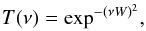 (2)where ν is the frequency in cycles per day, and W, the width parameter of the smoothing window, is here and throughout noted in units of day. The width parameter W characterizes the effective length of the filter in the time domain, and correspondingly, δν = 1 /W is the bandwidth in the Fourier domain. If the band is very narrow, then the corresponding W parameter is quite large, and straightforward filtering (convolving) in time domain becomes time consuming. By using the Fourier transform method implemented as fast Fourier transform, the computing time is significantly reduced.
Our method is equivalent to smoothing the original data with a Gaussian window in time domain (used, e.g., in Ball et al. 2014). The particular method of parametrization is chosen so that the corresponding smoothing effect can be easily compared with traditional moving averaging. The Fourier smoothing width W is therefore comparable to the W-day moving average. In Fig. 1 we show the transmission functions of three different smoothing filters: a local linear fit, a running average, and a Gaussian filter with the width W = 7. The frequently used moving-average filter clearly has several parasitic sidebands, the local linear fit has one sideband, and the Gaussian filter lacks any sidebands. From this it follows that the moving average is not the best device to cut off high-frequency noise or separate different frequency bands in time series. The downweighted local linear fit method (which is also a widely used smoothing method) approximate transmission curve is quite similar to the Gaussian having only minor extra transmissions in the region of the higher frequencies.
 |
Fig. 1 Three different transmission curves for a specific width of the time domain filter. |
The Gaussian-smoothed versions of the particular input proxies are denoted by E [W,0], where W is filter width parameter, and the zero as the second parameter stands for no offset applied; this parameter is non-zero for the passband filters introduced in Sect. 3.4. For generality, we also use the notion E [0,0] (t) = x(t) for the original signal. The detrended version of the input proxy x(tj)−E [W,0] (tj),j = 1,...,M is denoted by Ed [W,0]. Detrending allows us to emphasize the features in the high-frequency regions of the data.
3.4. Bandpass filtering
The smoothing process itself is a low-pass filtering in terms of signal processing theory. In the context of the Fourier transform method, we can also consider the so-called bandbass filters. The transformed signal is multiplied by a transfer function that consists of two symmetrically placed passbands. We used the simplest bandpass filters with the transfer function 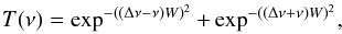 (3)where Δν = 1 /O is the passband offset. Below we use two parameters for bandpass filtering, the width parameter W, and the offset parameter O, both measured in days. The O parameter is essentially the period of the waveforms that pass through the filter unchanged (it determines the positions of the two maxima of the transfer function). For the bandpass-filtered time-dependent regression components we added the O parameter to the general expressions – E [W,O] (t).
 |
Fig. 2 Two different transmission curves for bandpass filters. |
In Fig. 2 we plot the two transmission curves for the bandpass filters. We used the differently filtered time series as regression predictors, which means that the exact normalization of the transfer functions is not important. The amplitude differences are absorbed into regression coefficients.
3.5. Envelopes
When we smooth the input data with different smoothing window parameters Wi,Oi,i = 1,... we obtain a set of curves that we can use as components for the regression modeling. For instance, if we systematically build a set of smoothed curves with offsets Oj = 1/(j·δν0),j = 1,...,J where δν0 is the frequency step, then by choosing proper δν0, we can well approximate the method of convolution kernel fitting, see, for instance, Preminger & Walton (2005). The important point here is that regression on smoothed components or approximation by moving kernel (convolution) are both fully linear procedures, that is, the predictions depend linearly on input data or smoothing kernel values.
To widen the range of modeling possibilities, we introduced a mild nonlinearity into our components. This allowed us to take the “sidedness” of the involved correlations into account and to move information along the frequency axis. This is useful, for instance, when the faster changing blanketing effect of the sunspots should influence the much slower changes in the overall network brightness.
One of the simplest nonlinear transforms of this type is the computation of envelopes. In this approach, we filter the input data set with a bandpass filter (e.g., with parameters W = 300d and O = 27d) and then compute upper and lower envelopes for the filtered data (see Fig. 3). The envelopes take the sidedness of different effects into account. They are also significantly smoother (shifting information in the Fourier domain from high to low frequencies).
There are many methods to estimate smooth envelopes but one of the simplest one is a spline interpolation through maxima (or minima). This is the method used in this paper. As seen from Fig. 3 the sets of the extrema are well defined for the band-pass filtered signals.
Our method is somewhat similar to the method of empirical mode decomposition that has been used in the same context (see, e.g., Barnhart & Eichinger 2011; Li et al. 2012). For the various components we obtained by bandpass filtering, we can find rather similar intrinsic mode functions. However, we prefer the somewhat simpler Fourier analysis approach because here the spectra of the important modes are highly concentrated in the frequency domain. In the solar context at least part of the variability is coherently clocked by the rotation. Quite close to our approach, at least from the methodological point of view, is the use of so-called wavelets and cross-wavelets (see, e.g., Benevolenskaya et al. 2014; Xiang 2014).
Rypdal & Rypdal (2012) used amplitude detrending together with mean deterending to reveal stationary (or statistically stable) fluctuations. Envelopes, as we introduced above, can be used with the same goal.
 |
Fig. 3 Fragment of bandpass filtered PSI data set E [W,O] (t) with upper E+ [W,O] (t) and lower E− [W,O] [t] envelopes. The envelopes are much smoother and have a sidedness that can take correlations or anticorrelations into account. |
 |
Fig. 4 Fragment of bandpass-filtered PSI data set E [W,O] (t) (thin curve above), its upper envelope E+ [W,O] (t) (thick curve), and the corresponding detrended version |
=E[W,O](t)-E^{+}[W,O](t)$}](/articles/aa/full_html/2017/04/aa27816-15/aa27816-15-eq45.png)
For the different smoothed (filtered) time-dependent data sets we used the following simple notions: E [W,O] (t) for bandpass filtered data, E+ [W,O] (t) for the upper and E− [W,O] (t) for the lower envelopes. The additional index d for E means that instead of the smooth envelopes of the curve being involved, they are used to detrend the bandpass-filtered data, or formally =E[W,O](t)-E^{+}[W,O](t)$}](/articles/aa/full_html/2017/04/aa27816-15/aa27816-15-eq49.png) for detrending with an upper envelope (see Fig. 4).
for detrending with an upper envelope (see Fig. 4).
Correlation matrices for input proxy data sets.
After defining our rather simple tool set of low-pass filtering (smoothing), band-pass filtering, envelope building, and detrending, we demonstrate their usefulness below in various data processing contexts.
4. Diagnostic tests
Using the simplest smoothing and detrending operators, we can obtain some insight into the physical characteristics of and problems related to different input proxy and target data sets. First we divide the data sets into two different parts, a smoother LF part, and a faster changing HF part. By systematically correlating these smoothed or detrended parts, we can better characterize the potential problems with data. Then we use parameter-dependent bandpass smoothing to build spectra that help to localize correlating and anticorrelating frequency bands of the data sets. These two simple exploratory type diagnostic tests allowed us to set up the general scene for the further investigations below.
4.1. FDCs of proxies and targets
The proxy and target time series all have prominently visible changes over distinct frequency ranges: a short-term variation, changes over the scale of the solar cycle, and possibly also some secular trends. To start, we therefore used simple Gaussian smoothing with the width parameter, W0, for all data sets to separate the signals into an LF and an HF component. The LF component is an input proxy data set smoothed with the Gaussian filter E [W0,0] (t), and the HF component is its detrended variant Ed [W0,0] (t) = E [0,0] (t)−E [W0,0] (t). The limiting width W0 = 750 was chosen using an optimization procedure of the first (and most prominent) components of the different regression models (see Sect. 5 for a detailed analysis). The results do not depend very much on this particular choice (we tried values between 500–1000 days). For simplicity, we call the W parameter in this simple analysis scheme a “breakpoint” and the LF part of the data sets a “backbone”.
First we examine the correlation matrices between the various proxy data, correlating the original proxies without smoothing, and the LF/HF parts separately; the results are presented in Table 2. The LF components of the proxies are very highly correlated (Rc = 0.982−0.998), even those that describe very different features (e.g., PSI vs. MGII). In other words, they can confidently be treated as interchangeable. This is not so for the HF part correlations: while PSI and SA correlate strongly with Rc = 0.894 (because they are essentially only slightly different measures of the spotedness), the correlation between the SA and MGII index, for example, is significantly lower (Rc = 0.521). In physical terms we can see that all the proxies describe essentially the same smooth (LF) change in the activity level, but the HF fluctuations are different, especially when the two different types (blanketing vs. brightening) of proxies are compared. This simple insight is used below, where we build different target approximations from proxy-based components.
Next, we investigate the correlations between the target curves with the same technique, and present our results in Table 3. As evident from this table, the structure of the correlations between the targets is different, the almost perfect correlation of the LF backbone seen in the proxies has significantly decreased for the targets. The range of variability is rather similar for all three comparison sets. For the original target data sets the correlation range is 0.861−0.937, for the LF parts it is 0.849−0.917, and for the HF components it is 0.906−0.957. For the PMOD-RMIB pair the HF correlation is somewhat higher than for PMOD/RMIB-ACRIM, which is also expected because PMOD and RMIB are based on the same measurements. The stronger differences in the LF backbones in Fig. 5 reflect issues in the TSI composite building, caused for example by the different methods used to take the instrument degradation trends or improper stitching of the observed fragments into account (see Kopp 2014 for the assessment of problems involved). This main controversy is an expected result, but we here express it explicitly and demonstrate the effects it has for model building.
 |
Fig. 5 Main controversy. To recover TSI for the past dates, we need reliable current estimates for calibration. The LF parts (obtained with a Gaussian smoothing filter with W0 = 750) of three target TSI composites differ significantly, however. The curves are shifted to a common level at 1996.465. |
Correlation matrices for input target sets.
The difference of the LF/HF behavior for the proxy and target data sets is crucial. It shows that regardless of the linear combination methods we use, the set of simple proxies is not sufficient to properly describe all the target sets. The rather large variability in the LF components of the target sets needs additional arguments to be explained and potentially requires additional data to determine which of them should be used for proper TSI reconstruction and hindcasting.
 |
Fig. 6 Scatter plots for PSI-PMOD pair: a) – linear fit of the proxy to data (Rc = 0.020); b) – regression modeling using the simple model (Rc = 0.860); c) – multicomponent model (Rc = 0.893). |
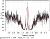 |
Fig. 7 FDCs between overlapping parts of the PMOD and PSI data sets as function of the band-pass offset Δν. Width |
4.2. Narrowband FDCs
It is well known that traditional activity indicators (e.g., sunspot numbers) are not well correlated linearly with the TSI measurement series (see, e.g., a recent demonstration by Hempelmann & Weber 2012). In Fig. 6a we present a typical scatter diagram, in this case between the overlapping parts of the PSI and PMOD data. We can try to build nonlinear regression curves between these two, but the predictive power of this type of relations is very low (Preminger & Walton 2005; Zhao & Han 2012; Hempelmann & Weber 2012).
With a proper filtering and data analysis technique, we can characterize our input data sets (e.g., PSI as proxy and PMOD as target) in terms of the FDCs. This means we do not correlate original data sets, but various parts of them in the frequency domain. For this purpose, we filter proxy and target curves with bandpass filters with different frequency offset parameters and correlate the results (by computing standard Pearson correlation coefficients Rc). In Fig. 7 we show the results of such a simple computation. The filter width parameter W = 2000 was chosen so that enough detail would be revealed. This value is a good compromise between frequency resolution and lower signal-to-noise ratio that is due to the narrowness of the filter. The spectrum for W = 30 is discussed below. Figure 7 clearly shows that different parts of the spectrum correlate in different directions. First, there is a strong central peak with a high positive correlation that arises from the highly correlated LF components. Then there is a wide band up to the frequencies approximately 0.1 cycles per day with a strong anticorrelation. From 0.1 to 0.2 a transient band is visible where the correlations are still negative, but no longer strong. Finally, our “spectrum” starts to wildly oscillate around the zero level correlation. The region of negative correlations also shows separate “spectral lines” with a weaker anticorrelation. The most prominent of these lines occurs near the solar rotational frequency ν = 1/27d-1. This shows that the method of FDCs is rather sensitive to various aspects of the TSI variability (in this case, to solar rotation).
The quite simple experiments with smoothing and bandpass filtering allowed us to reveal interesting aspects of the proxy – target relations. A more systematic approach demands introduction of certain regression schemes.
Motivated by the results of the diagnostic tests above, we build below different regression models of the type of Eq. (1).
5. Simplest regression models
Because our approach contains a number of new techniques and notions, it is useful to describe their application in a sequence of steps, starting from the simples ones, and finally showing the final results. We start from the model where only one smoothed component, the original proxy, and a constant level are used as regression components. Moreover, hereafter we only consider proxies related to the blanketing of sunspots (SA, SN, and PSI), and therefore we do not directly model the facular brightening component (that could be described, e.g., by MGII and LYMAN data sets). One important argument for this neglection arises from the shortness of the facular proxies, due to which they have a limited hindcasting capacity. During our step-by-step approach, even without the facular component, our methods yield a modeling power comparable to the physics-based models that include the brightening component.
This simple model can be useful as a poor man’s modeling device.
5.1. Three-component model
The FDCs plot in Fig. 7 shows two main features: a highly correlated LF part (peak at the center), and a wide anticorrelated band at higher frequencies. Based on these characteristics, we assume that the following regression model can be used to approximate the TSI using a proxy: +a_2 E[W,0](t), \label{simplemod} \end{equation}](/articles/aa/full_html/2017/04/aa27816-15/aa27816-15-eq71.png) (4)where we use the general notions E [0,0] (t) for the original proxy and E [W,0] (t) for its smoothed variant. The smoothed component should correlate with low frequencies of the target curve, and the second term, with the coefficient a1,a1< 0, should account for the anticorrelations. The parameter values of the model C(t) were obtained by combining linear least-squares minimization for coefficients a0, a1 and a2 with an exhaustive grid search for parameter W. The results for a concrete example of the proxy/target pair, PSI vs. PMOD, are listed in Table 4.
(4)where we use the general notions E [0,0] (t) for the original proxy and E [W,0] (t) for its smoothed variant. The smoothed component should correlate with low frequencies of the target curve, and the second term, with the coefficient a1,a1< 0, should account for the anticorrelations. The parameter values of the model C(t) were obtained by combining linear least-squares minimization for coefficients a0, a1 and a2 with an exhaustive grid search for parameter W. The results for a concrete example of the proxy/target pair, PSI vs. PMOD, are listed in Table 4.
Regression model in standard format for the PMOD target built using PSI as a proxy.
The prominent feature of the simplest solution is the minus sign for the coefficient a1, which means that the original non-smoothed component enters into the model in a reversed way, while the smoothed component enters with a positive coefficient a2. In the context of our study, this is quite understandable because the spots serve as radiation-blocking elements on the solar disk. The overall level of solar magnetic activity is modeled by the smoothed with W = 792 component. Our simple model convincingly demonstrates how the correlating and anticorrelating elements of the input curve can be separated by using Gaussian smoothing with a properly set smoothing window width.
In Fig. 6b we show a scatter plot of the observed TSI (PMOD composite) and our simplest PSI-based regression model, showing a prediction modeling precision at correlation level Rc = 0.860. As evident when comparing with the correlation matrices for the targets in Table 3, the obtained value is practically the same as some correlations between targets (e.g., ACRIM vs. PMOD at Rc = 0.861). Consequently, at the current level of observational precision, the errors brought in by the modeling procedure are not significantly higher than the variations between the input data sets.
This urges us to proceed to other computational experiments.
5.2. Baron von Munchausen method (BvM)
Because our knowledge about the directly measured targets is controversial in the sense that their LF parts differ significantly, we assume that we can precisely estimate the real target TSI values with the following data manipulation method, which we call Baron von Munchausen method (hereafter BvM): we take the TSI curve estimated from regression modeling (e.g., of the PMOD), subtract its LF component, and add the LF component of the actual target. This means that we try to ignore the errors that are due to the improper modeling of the LF part of the TSI. In the particular case of modeling PMOD using PSI as a proxy, we obtain the following result: while the resulting model correlation for the real data is Rc = 0.861, for the combined curve in which the LF part of the regression model is replaced with the LF part of PMOD (BvM), it increases to Rc = 0.887, see Table 6. This is the potential prediction accuracy level for the simplest model for the particular case when the following two conditions are fulfilled: the LF part of the target TSI is measured correctly, and the LF part of the target TSI does not contain any secular components (all its variability is strongly connected to the magnetic tracer statistics).
In Fig. 8 short fragments of the target data set PMOD, of the predicted curve, and of the BvM-corrected curve are plotted to show that the PSI curve, if mapped properly, can model PMOD as target. The part of the residual differences originates from the brightening events that are not accounted for in sunspot statistics and/or do not correlate with it. Another difference is due to the unavoidable modeling errors. In Fig. 9 we plot the LF parts of our reconstruction based on the simple model (Eq. (4)) and the target PMOD. The difference between these curves is only the BvM correction we applied to our solution to form an idea how precisely short timescale fluctuations in the TSI curve can be modeled by the raw PSI data.
To recapitulate this part of the analysis: the raw PSI data used as a straightforward blanketing model combined with correct LF part helps us to achieve regression modeling precision at the level of Rc = 0.887 (PSI vs. PMOD) or Rc = 0.898 (PSI vs. ACRIM), which is indeed quite high. For the hindcasting problem this is important. We do not have proper data to estimate the daily brightening component for the historical data, but this may not be very important. For the proper LF part, the raw PSI data as a regression component are very useful. In the next section we further improve on this by using additional PSI (or other proxy) -based regression components.
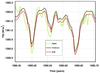 |
Fig. 8 Fragment of the simplest prediction from PSI to PMOD together with the BvM version and the target PMOD data. |
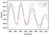 |
Fig. 9 LF parts of the simplest prediction using PSI as the proxy and PMOD as the target. |
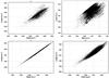 |
Fig. 10 Correlations between PMOD and ACRIM and regression models based on them (using PSI as the proxy): a) cross plot of the original target data sets PMOD vs. ACRIM (Rc = 0.861); b) cross plot for the solution without restrictions (Rc = 0.512, Fig. A.1, see Appendix A.); c) cross plot based on the simplest models (Rc = 0.998); d) cross plot between restricted multicomponent models (Rc = 0.941). |
5.3. Application of the simple scheme
We then applied the simple regression scheme described by Eq. (4) to all the different sunspot-tracing proxy-target pairs. In Table 5 we list the optimal breakpoint W values for different pairs. These values tend to be rather similar between all the targets. The correlation levels achieved by using the simple prediction scheme are given in Table 6. In this table, we present two types of results: in the first part (simplest scheme), we list the correlation values between the simplest model prediction and real data. In the second part (BvM), we display correlations obtained by our BvM scheme with the backbone substitution.
Optimal W values (breakpoints) for the simplest models.
We computed TSI hindcasts for every proxy-target pair and compared them by computing correlation coefficients between the different solutions. The four-dimensional correlation matrix obtained for different proxy-target pairs is given in Table B.1. Different solutions are inherently quite consistent. This is also demonstrated in Fig. 10c. for the particular combination PSI-PMOD vs. PSI-ACRIM. The similarity of almost 100% between the two hindcasts results from the fact that all information about the targets is compressed into only four estimated coefficients: the linear parameters a0, a1, and a2, and the nonlinear smoothing parameter W. If we take into account that the correlation computation itself balances out two of them (mean level and dispersion), then we are left with only two parameters.
The correlations between targets and the prediction fragments are significantly more scattered for different proxy-target pairs (Table 6). Part of this scatter is a result of our rather trivial modeling method (raw proxy as a model for blanketing). The other part is due to the different predictive capacities of the proxies (e.g., PSI vs. SN). Finally, the large spread of different target values also influences the prediction and hindcasting outcomes.
Nevertheless, the correlation levels achieved using this simplest scheme (e.g., 0.860 for the PSI-PMOD pair) are rather high. The corresponding hindcast TSI curves can well be considered as simplest solutions for the hindcasting problems. The much more complex models described next increase the level of proxy-target correlations, but also loose some robustness and stability.
6. Multicomponent regression models
The simplest regression models described above only take two important features of FDCs into account (see Fig. 7): the central LF peak, and the wide anticorrelation depression. To account for narrow peaks in this spectrum, we need to add components to our modeling scheme. This is a far from trivial task. Of the large set of trial components, only a small number are useful: they help to model the target and are stationary enough to have a predictive capacity. This forced us to include various selection and restriction steps in our final hindcasting algorithm.
Prediction vs. target correlations for the simplest regression model and for the BvM variant of it.
6.1. Model building
The simple regression scheme can be improved by adding some new components to the simplest model: +a_2 E[W,0](t)+\sum_{l=3}^L a_l E_l[\dots](t), \label{fullmod} \end{equation}](/articles/aa/full_html/2017/04/aa27816-15/aa27816-15-eq96.png) (5)where El [... ] are different transforms of the proxy data. Using added components, we tried to model finer details, as we show in Fig. 7. For instance, in the region of the rather broad frequency offset band of strong anticorrelations, some peaks with significantly weaker anticorrelation/almost complete uncorrelation can be found at approximately the frequency offsets corresponding to solar rotation.
(5)where El [... ] are different transforms of the proxy data. Using added components, we tried to model finer details, as we show in Fig. 7. For instance, in the region of the rather broad frequency offset band of strong anticorrelations, some peaks with significantly weaker anticorrelation/almost complete uncorrelation can be found at approximately the frequency offsets corresponding to solar rotation.
To build new trial components, we filtered the proxy data set with different bandpass filters, allowing the width, W, and the frequency offset parameter, O, to vary. We also applied different envelope construction modes.
The full multidimensional least-squares optimization over a large set of parameters and envelope-building modes is very time consuming. We therefore used a suboptimal modeling method, the so-called greedy algorithm. In every step of this algorithm we introduce a new component from the full library, include it in the overall regression model, and optimize it to obtain new values for the width and offset parameters. The values W and O and the envelope mode that result in the best final correlation are then taken as parameters of the component to be included. In principle, this stepwise inclusion of the new components can lead us away from the best solution. The probability for this to happen, however, can be regarded as low because the features in the correlation spectrum tend to stay apart, and consequently, the sequential components are nearly orthogonal (they do not correlate strongly with each other). Even if some presumably incorrect component is accidentally included, the possibility remains that its effect is decreased by some components that are added later. The overall scheme is very similar to the cleaning approach in a frequency analysis (see Roberts et al. 1987).
For the model building the full library contains an almost complete set of components (in principle, the target curve can be matched almost perfectly), but most of the low-amplitude components do not have any predictive value: they model either noise or other contingent aspects of the target (see, e.g., Fig. A.1). For practical as well as conceptual reasons, we therefore need to stop somewhere. In this work we chose to include components up to the moment where the increase in corresponding correlation level between proxy and the target is lower than 0.001. This choice is reasonable because, as we show below, the set of really interesting components (from the point of view of predictive power) is rather low.
Unfortunately, as shown in the counterexample (Tables A.1, A.2, and Fig. A.1) a straightforward application of the greedy search method significantly improves the fit between the model curve C(t) and target Y(t) (for the PSI–PMOD pair Rc = 0.906, for the PSI–ACRIM pair Rc = 0.918), but it produces very unstable solutions for the hindcasting problem. Therefore we need to carefully consider which components are useful for the actual hindcasting.
6.2. Selection of regression components
To achieve more stable proxy – target hindcasts, we need to carefully select the regression components. Here we applied three different methods to ensure we discard unwanted variants of the different proxy transformations:
-
For the component-seeking procedure we preprocess input datato remove LF backbones from the proxies and from the targets. Inthis way, new components will model only HF correlations; seeSect. 6.2.1.
-
We check the predictive power of the new components by trial prediction within the available data, see Sect. 6.2.2.
-
We also consider the physical plausibility of the components by constraining certain parameter values, see Sect. 6.2.3.
All three methods are fully automatic, and no manual intervention is applied.
6.2.1. Preprocessing
For every proxy-target pair under study, we first built the simplest prediction model as described above. Then we used the optimal smoothing parameter W from the simple model (see Table 5) to divide the input data sets into LF and HF parts. By subtracting smoothed variants from the input data, we essentially removed the effects of the LF correlations (central peak in Fig. 7). The remaining HF parts were then used in the component-selection process as input data. This preprocessing procedure allowed us to avoid a leakage effect where the LF parts influence HF parts and vice versa. A division into smooth and fluctuating parts such as this is often used (see, e.g., Rypdal & Rypdal 2012) but the breaking point is often chosen arbitrarily. Here we determined it with the optimization procedure. When components were selected from HF parts, they were included as predictors into the final regression model to evaluate their relative strengths.
6.2.2. Cross prediction
To distinguish between the simple goodness-of-fit and the prediction potential of the components, we divided all HF parts of the input data sets into two parts I and II with equal lengths in time. The first part covered approximately cycles 21–22 and the second part cycles 23–24. In every new component-seeking step we then evaluated a fit criterion in the following way. For every possible parameter combination, we built two separate models: for the first, I, and for the second part, II, of the data. Then we used these models to predict or hindcast the other one. In this way, we obtained two correlation values,  and
and  where T denotes the particular type for the envelope (upper, lower, or simple smoothing, detrended or not). It is important that the model parameters in this procedure were computed using one part of the data but the correlation is measured between the predicted values and the other part. For each parameter set, we then took the minimum value for the two correlations and maximized it to derive proper parameter values. Formally, we chose
  (6)as our final correlation estimate for a particular component. In this way, we selected components that may be ill-suited for detailed modeling, but perform well in the context of predictions.
6.2.3. Search domain restrictions
There is an additional method to cull components that can lead to incorrect predictions. Pelt et al. (2010) showed that the magnetic activity on the solar surface has a certain “memory” that is somewhere around 7–15 solar rotations. This means that modes whose wavelengths are longer than a given value can describe accidental correlations, not systematic ones. Therefore it is reasonable to restrict the parameter range for bandpass-filter offsets to values O< 500 days. We assume that dependencies with longer wavelength correlations are previously absorbed into the LF components or do not contribute as potential sources of predictive power.
On the other hand, it is also reasonable to restrict the W parameter. Values of W that are too high result in bandpass filtering with very narrow bands, and consequently, the corresponding envelopes are prone to fluctuations (the spectral information for these modes comes from only small set of the Fourier-transformed data values). There is no good quantitative method to derive this limit from the physical principles, but from the wide range of trial computations with different input data sets, we found that the limit W< 2000 can well be used as a reliable approximation.
By combining cross prediction with the restrictions for the model parameters, we now have a method to model HF parts of our targets and then to hindcast past TSI values. It is quite clear that this method will provide a lower overall fit quality than the two examples given in Appendix A, but it is expected that the hindcast quality will increase.
6.3. Computed models
Our final regression model for the hindcasting of a target using a proxy then consists of (the parameters that are to be estimated are added in parentheses):
-
constant level (a0);
-
the proxy curve itself (a1);
-
an optimal LF component (a2);
-
set of components from the HF analysis (a3,...).
The typical component-seeking process is illustrated in Table 7 for the PSI-PMOD input data pair. First the values of the determined component parameters are given, and then the estimated regression coefficients. In the final two columns the convergence process of the iterations is illustrated by listing at each step the correlation level that has been achieved and its increment. Similar data for PSI-ACRIM pair are presented in Table 8. These tables show that all different solutions contain components with offset parameter values around O = 27d, which corresponds to the solar rotation, as Fig. 7 indicated. Similarly to the rotation signal, the components lie in the interval from O = 9 to O = 12 in the different solutions. These components appear because the method tries to take the features in the transient part (from anticorrelation to decorrelation) of the FDC spectrum into account. The remaining components describe low-frequency features and differ more from one method to the other. In principle, they absorb more contingent features of the variability, and consequently, they depend more strongly on the method that is used. Certainly the solutions based on cross prediction, even if they are slightly less correlated with the learning sets (targets), must be taken more seriously.
In Fig. 11 we plot multicomponent hindcasting solutions for the pairs PSI-PMOD and PSI-ACRIM together with the LF components of the target curves PMOD and ACRIM. The statistical correlation between the solutions is rather high (Rc = 0.941), but the curves differ somewhat. Subjectively, we would prefer the first solution, but according to the approach taken in this paper, we treat all solutions equally. This plot can be also compared with Fig. A.1, where unconstrained modeling results are depicted in a similar format. The introduced selection procedures for model components allow more stable solutions.
Modeling PMOD data using PSI as a proxy. Regression components and iteration progress.
Modeling ACRIM data using PSI as a proxy. Regression components and iteration progress.
The obtained correlation levels for the entire set of proxy-target combinations is presented in Table 9. In the first group of the table (HF prediction), we list the correlations achieved by modeling the HF parts of the corresponding proxy and target. The second group (Prediction) consists of the final correlations of the model, where both the component smoothed by optimal values of W and components found from HF analysis are included. And finally, as with simplest models, the third group displays correlations for the mixed models, where LF part is substituted by backbone from target (BvM method).
Achieved correlation levels for the multicomponent regression model.
Table 9 and Fig. 6c show that the correlation levels achieved using the multicomponent regression models lie between the levels of the simple prediction schemes and models to which components were added without any restrictions (see Appendix A). For PSI-PMOD pair the corresponding levels are 0.860 (the simplest method), 0.893 (multicomponent method), and 0.906 (unrestricted method). For the PSI-ACRIM pair the respective levels are 0.749, 0.796 and 0.918.
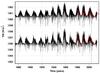 |
Fig. 11 Hindcasting based on multicomponent models. PSI to PMOD mapping (upper curve) and PSI to ACRIM (shifted down by five units; lower curve). In red we plot the low-frequency backbones of the target curves. The cross correlation between the two hindcast curves is Rc = 0.941 (see Fig. 10d). |
Probably the most striking result is the very similar correlation level that is achieved with the BvM method (see Table 9). From this it follows that all the three targets are practically equivalent when we consider their HF behavior (blanketing by sunspots and short-term enhancements). All the problems and differences between the targets originate from their LF behavior.
The actual predictions (Table 9, the Prediction part) differ more significantly. This is also illustrated in Fig. 10d, where the cross plot between the PSI-PMOD prediction and the PSI-ACRIM prediction is displayed. The correlation level is certainly better than with the unrestricted model solution (b), but this is far from being the case with the simple model (c).
In Fig. 12 we compare the prediction errors for the final multicomponent solution (upper panel) and the BvM variant of it (lower panel) that were computed for the PSI-PMOD proxy-target pair. The day-to-day error values in the plot are somewhat misleading because of the low resolution of the plot. Differences (errors) between monthly and yearly averages show the expected level of precision for the applications where such averages are used as an input. Unfortunately, the plot also demonstrates the level of ambivalence that is due to the main controversy, that is, to the varying LF behavior of the targets (the BvM method shows how the solution behaves when the LF part is adopted from the real data).
 |
Fig. 12 Prediction errors (absolute differences) between predicted curves and targets for the PSI to PMOD pair (upper panel) and corresponding BvM solution (lower panel). Black shows the daily errors, red the errors for filter curves smoothed by W = 30, and green the errors for filter curves smoothed by W = 365 . The data sets are nearly 14 000 points long, and consequently, the plot points essentially mark the local maxima of the curves (for each pixel). The scatter of the errors can also be characterized by their standard deviations: 0.169, 0.113, and 0.076 for the upper panel and 0.156, 0.090, and 0.025 for the lower panel. |
6.4. Postprocessing
After the hindcasts are built with different simple and multicomponent regression models, some refinements can be applied to the final data products.
The scatter of the correlation levels between PMOD and PSI (Fig. 7) strongly oscillates at higher frequencies. When we compute FDCs using a wider passband, for instance, setting W = 30 instead of W = 2000, we obtain a much smoother curve. From Fig. 7 we can see that the average level of correlations reaches the zero level only asymptotically. This means that we have certain minor correlations even for the very high frequencies. These correlations are due to the very sharp peaks in the time domain that have wide images in Fourier domain (this is true for targets as well as for proxies). However, because the statistical fluctuations are of general origin, they are practically useless. Even if we try to add many high-frequency modeling components, we end at certain overfit situation. Consequently, it is reasonable to cut out the high-frequency region from our prediction scheme. Figure 7 shows that a frequency of 0.2 cycles per day is a reasonable limit. The effect of this minor smoothing with a W = 5 Gaussian filter is not very dramatic. For instance, in the case of the correlation value Rc = 0.893 between the PSI vs. PMOD solution and the original PMOD (see Table 9, column Prediction), the correlation after smoothing both of the curves attains the level 0.9022. Therefore it is reasonable from a practical viewpoint to mildly smooth the final data products. Even if we claim that the obtained results are given as day-to-day data, the other users must be aware that some minor details are not presented in hindcasts, especially that the sharpest peaks are somewhat rounded at their extrema. Fortunately, most of the applications need only data on much coarser grids, and then these minor details are certainly averaged out.
Obviously, our methods do not help at all in the context of estimating the absolute level of the TSI even if this is an important aspect of the Sun-Earth relations (see Kopp & Lean 2011). However, for presentation purposes, we need a certain fixed point to tie the different time series together. There is one obvious candidate to clearly show the overall level of the TSI: the cycle 23–24 minimum (1360.85 Wm-2 at 15 October 2008 see White et al. 2011). However, this leads to a wide spread of targets for exactly the time when the Sun worked as usual. We therefore chose as a compromise another minimum between cycles 22–23 (1361.11 at 1996.465, see Fig. 5) using a similar smoothing method as in the original paper (White et al. 2011).
All the results are available in the form of simple text files that can be downloaded10. The predicted time series are all shifted to a common mean level and are mildly smoothed, as described in the last two subsections. The input data sets and modeling methods for every prediction can be read off from their file names.
7. Discussion
From the statistical point of view, the TSI consists of three components: variability that originates from a straightforward blanketing effect due to the sunspots, variability that statistically correlates with sunspot occurrences (or their areas), and residual variability. The last component contains long time trends of overall variability and short time features that occur randomly and are not statistically correlated with sunspot occurrences. Part of the residuals is also due to the nonlinear correlations, which are more complex than the correlations that are accounted for by modeling using smoothing and envelopes.
The method of FDCs allowed us to quantify these observations and to localize different aspects of variability in the frequency spectrum (for a more traditional description of the time variability, see the review by Solanki & Unruh 2013). From the physical point of view, we can classify the solar variability in even more detail. Every spatial disturbance in luminosity (regardless of spectral region) also translates into the time domain due to rotation. Evidently, this translation is far from simple: the different activity tracers are likely to have phase shifts and undergo phase mixing. Nor can the translation be expected to occur over one discrete frequency, as the rotation velocity depends on both latitude and radius of the Sun. In addition, we can have certain secular changes that result from the particular way the solar dynamo operates. The recent DNS model of Käpylä et al. (2016), which covers roughly 80 simulated solar cycles, suggest that prominent secular changes can indeed occur as a result of the existence of multiple dynamo modes with cycles of varying frequency. Even though the cycles seem to be rather regular in frequency, their interference can cause abrupt phenomena that are reminiscent of the Maunder minimum in addition to a smooth secular component.
As a result of our smoothing experiments with varying window width, we found that the strategically most important breaking point is localized at the frequency that corresponds to a period of ≈750 days. We used this dividing line to build LF and HF components of the proxies and targets. When comparing the LF parts of the proxies (PSI, SA, and SN), we can conclude that they are rather similar and essentially contain the same information. These curves characterize the slowly changing mean level of solar activity, which shows itself through the statistics of sunspot occurrences. The similarity of the LF component of the proxies is a hindrance for the use of multiple regression TSI models (see, e.g., Zhao & Han 2012), where different proxies are combined to obtain TSI estimates. The models can still be improved, however, by increasing the accuracy of the HF part description.
The LF parts of the target data sets (PMOD, RMIB, and ACRIM) differ more from each other. The differences between them originate from certain instrumental, data processing, and other method-related problems (Kopp 2014). For TSI hindcasting, the LF variability is the strongest hindrance because to recover TSI values in the past, we need a good understanding of the present-day values, which is currently unavailable.
The HF parts of the proxies differ because they are constructed from the observed data in different ways. The HF part is relevant for high-resolution prediction (up to daily accuracy level). Here the proxies can be ranked by their information content. The best of them is PSI, which, if used in a proper regression scheme, was shown here (and in earlier work) to describe a very large amount of target variability. However, if we need hindcasts extending farther back in time, then the SN becomes useful. How much information we loose by using these rough data can well be deduced from the above computations.
Using the Baron von Munchausen scheme, we demonstrated that the HF behavior of all three targets is very similar. For instance, after backbone substitution, the achievable correlation levels for the PSI proxy were in the narrow interval 0.908(ACRIM)- 0.914(PMOD) (see Table 9). This similarity is of course the result of the essentially common origin of all the three target data sets. The main differences among them come from different methods of fragment stitching, not so much from rescaling or interpolations.
Probably the most unexpected result of the current analysis is the relatively high prediction capacity of the simplest models. For instance, the simple model prediction for the PSI-PMOD pair correlates with the target at the level Rc = 0.860 (or, in other words, describes a 74% of variability). For 30-day running means of the target and predicted curve, the correlation level is already Rc = 0.924 (85%). Consequently, if we trust any of the TSI compilations (e.g., PMOD), then we can extend it into the past with reasonable confidence. In essence, the simplest method consists of estimating one nonlinear parameter W and one ratio between amplitudes (the LF part and the original proxy). The other nice property of the simplest scheme is the inherent consistency of the different solutions (see Table B.1).
In the simplest models we involved only two aspects of the proxy variability: the LF part as a model for the smooth overall activity variation, and the original proxy as an approximation of the blanketing effect by sunspots. There is certainly an amount of variability that is not yet accounted for (brightness enhancements, etc.), and therefore we can extend the simplest models by searching for more regression components. From the wide library of the possible modes, we selected those whose parameters lie in the physically plausible ranges, which have the capacity to predict from one part of the series to the another and which bring significant improvement to the final correlation between the predicted curve and target. This procedure of building these multicomponent models is rather time consuming and unfortunately not very productive (for the particular set of proxy-target pairs). The final increase in correlation levels between simple and multicomponent models is only around 3−4%, and we pay for this increase with a widening spread between different solutions. For instance, the maximal spread between different proxy-target solutions (see Table B.2) is 0.8879−0.9836. We can compare this with the range for simple models 0.9957−0.9997 (Table B.1). Of course, this is expected. To calibrate the simplest model, we used only two adjustable parameters that are computed from the targets. For multicomponent models, the set of adjustable parameters (regression coefficients) was significantly larger. The discrepancies between different target curves (our main concern) are transported into the solutions for predictions and cause them to spread out. As we showed in the example with unrestricted models (see Fig. A.1), the spread can be even wider when we ignore physical constraints and the prediction capabilities of the different modes.
The low degree of improvement achieved by including additional components can also be explained by the low level of actual correlation between day-to-day values of the two components of the TSI variability: blanketing due to the sunspots and brightening due to the faculae. The LF behavior of these two components can be rather similar as they result from the occurrence and disappearance of the active regions. Nevertheless, their HF behavior is different.
7.1. Particular proxy-target pairs and expected precision of hindcasts
The backprediction precision of model-based hindcasts can be estimated only very approximately. The computational and statistical errors (e.g., due to the estimation of regression coefficients) are significantly lower than the overall spread of different solutions, so that it is not even reasonable to tabulate them. The entire spread of the solutions originates from different input data sets and from differences in regression model compositions.
There are some components that are quite similar for all the 3 × 3 = 9 models. The breakpoint parameters W (Table 5) for different proxy-target pairs lies in the interval 472.7−825.8 days. The smoothness of the corresponding backbones is visually rather similar, and their differences (if relevant) must reveal themselves in slightly different additional modes.
Another similarity between the different models occurs near the solar rotation period. All component sets contain a mode with a period of approximately 27 days and with a width parameter W ≈ 400 days. This component suppresses the effect of the proxy in the narrow uncorrelating band near the solar rotation (see Fig. 7).
The third set of common components is around parameter values W = 10 and O = 10 days. These components try to filter out the high-frequency regions that are decorrelated.
The remaining components can be common for some proxy-target pairs, but can also be lacking in other sets. They model the more contingent properties of certain combinations. A large part of the differences between the obtained solutions stems from these components.
We can also compute correlations between different predictions. From the 9 proxy-target pairs we can obtain 36 pair-pair comparisons (Table B.2). The most similar pairs are PSI-PMOD and PSI-RMIB (Rc = 0.984), and the most different are SN-PMOD and SA-ACRIM (Rc = 0.804). These two numbers can probably also be used as limits for very conservative (and naive) estimates for retrodiction precision.
Of course, if there are reasons to prefer some particular proxy-target pair, the outlook is not so bleak (see Table 9). The current state of affairs is very strongly affected by the main controversy, that is, by the discrepancy between various targets.
However, it may be possible to obtain somewhat more precise predictions. This comes from the other approach of TSI approximation. Namely, we can use SATIRE-S-type physics-based models (see Ball et al. 2012) as targets in our prediction scheme. In this case, we know the actual building blocks of the TSI approximation and can use this information for proper prediction. We leave this approach for the next iteration of our research program.
7.2. Effect of solar rotation
Sun-like stars show an unexpected damping of correlations around the solar rotation frequencies, which may confound using our method in this field of research. Even if for some simple models (see, e.g., Lanza et al. 2007), we can see some localized correlations over a certain frequency, then for the full solar data (e.g., PSI against PMOD), there is a quite wide peak of very weakly correlating frequencies. Put simply, the straightforward blanketing (PSI) does not reveal itself strongly in TSI curves (PMOD) when observed through a narrow frequency band filter. Even if small day-to-day details coincide rather well (Fig. 8), the reshuffling of events along rotation phases and their mixing with more random facular changes results in a strong decorrelation. We consider this aspect of our investigations very important and will work out more details in the next paper of this series.
7.3. Restrictions
Our constructions are all based on the assumption of statistical stationarity. However, it is well known that the solar magnetic activity has undergone some rather abrupt states of lower activity (grand-minima-type events). Some of these events may be the result of the chaotic nature of the highly nonlinear physical system (see Zachilas & Gkana 2015, and references therein) or might be caused by the interference of various dynamo modes with different spatial distributions and symmetry properties with respect to the equator (Käpylä et al. 2016).
It is not ruled out that the currently available set of TSI estimates (targets) contains a certain breakpoint when the Sun changed its normal mode and switched to a new regime. In the cross prediction scheme above, we combined backward and forward predictions to distill variability modes that change consistently over the full time. If the two parts differ strongly in their statistical behavior, however, then only a small number of variability components can be persistent enough to allow their use away from the calibration zone. In this case, our method is not as effective as it could be in the stationary context. It is also well known that other Sun-like stars tend to show rather complex long-term patterns (see, e.g., Oláh et al. 2012), in which case it is not ruled out that the interval of the solar cycles 12–23 was a calm intermezzo of regularity.
Another restriction is the time symmetry of the assumed correlations, that is, the variability modes are selected only using frequency slots and no time delays are involved. However, some processes on the Sun can have an asymmetric statistical nature in time. For instance, the disintegration of activity complexes is one such process. Li et al. (2010) conjectured that in the relation of sunspot activity to the TSI, a 29-day time lag is involved. In principle, it is possible to extend our component library with modes shifted in time, but this greatly increases the model search space.
Similarly, the proxies enter the models linearly, but it is well known that in some cases a nonlinearity along proxy values (not in time) can be instrumental (see, e.g., Hempelmann & Weber 2012). The extension of the component library in this direction would be computationally costly, and therefore it is beyond the scope of this study. Different types of (implicit) nonlinearities can be accounted for by using neural networks approach (see, e.g., Tebabal et al. 2015).
As we showed above, the LF components of different proxies (long and shorter) correlate so strongly that it is not reasonable to combine many of them into a regression scheme. However, the situation is different with the HF parts. Here some of the proxies depend more on blanketing and some more on brightening events. By combining some of them into a general regression model, we can achieve better modeling precision (see for a similar approach Woods et al. 2015). Unfortunately, all the long proxies that are suitable for hindcasting belong to the group that only depends on sunspot statistics, no flares or similar phenomena are accounted for. Consequently, the FDC method with multiple proxies can only be used for more precise interpolation and stitching of the recent data.
7.4. Applications
The proposed scheme of building prediction models from proxy data sets has many additional applications. The main application naturally is the hindcasting or true prediction. However, we foresee some other important applications as well. First, the scheme can be used to fill in gaps in some observed target data by using those parts of the data where the proxy and target are both available to build a prediction equation according to which the gaps are then filled based on the proxy. The improved data set obtained through this procedure can iteratively be used for further refinement of the prediction scheme until convergence is achieved.
The second important application of the new scheme is stitching together target data from many sources, for example, from different satellites. In this case, we can develop a bridging scheme for fast-changing parts of the input data using all the observation sets. Then the low-frequency smooth components can be levelled off by bending them along the low-frequency part of the proxy curve.
In some other situations the prediction scheme can be used to reveal secular trends or outliers in the data. We can build proxy to data bridge using all or the most typical fragments of the observations. After that, the differences between predicted and observed values can reveal trends or outliers.
8. Conclusions
We have introduced a rather simple computational scheme that uses bandpass-filtered signal components as building blocks. The practical use of these components allowed us to reveal a set of rather interesting aspects of the proxy-target relations in the traditional context of TSI reconstruction and hindcasting. First we confirmed (in quantitative form) with an optimized smoothing procedure that the most serious problem of TSI treatment is the very large variance between the low-frequency parts of the existing TSI composites. Then we demonstrated a rather paradoxical feature in proxy-target pairs, namely that the solar rotational signal is not strongly manifested in the targets and proxies, but it is clearly and strongly visible in the frequency-dependent correlation spectrum. Finally, we proposed a computational scheme for building TSI models that use the well-known proxies as input data and are calibrated against currently available estimates of the irradiation levels. The introduced modeling method can be used in different contexts: gap filling and interpolation, stitching of observed data fragments, and in retrodiction and prediction schemes. Hindcasts computed with the new method can be useful in climatological models for about the past 200 yr.
Acknowledgments
We are thankful to late Olavi Kärner, who suggested the problem to us and referee for her/his useful comments. We also thank Frederick Gent, Natasha Krivova, Jyri Lehtinen, and Sami Solanki for helpful discussions. This work has been supported by the Academy of Finland Centre of Excellence ReSoLVE (Grant No. 272157; J.P., M.J.K., N.O.) and by the Estonian Research Council (Grant IUT40-1; JP).
References
- Ball, W. T., Unruh, Y. C., Krivova, N. A., et al. 2012, A&A, 541, A27 [NASA ADS] [CrossRef] [EDP Sciences] [Google Scholar]
- Ball, W. T., Krivova, N. A., Unruh, Y. C., Haigh, J. D., & Solanki, S. K. 2014, J. Atmos. Sci., 71, 4086 [NASA ADS] [CrossRef] [Google Scholar]
- Balmaceda, L. A., Solanki, S. K., Krivova, N. A., & Foster, S. 2009, J. Geophys. Res. (Space Phys.), 114, 7104 [Google Scholar]
- Barnhart, B. L., & Eichinger, W. E. 2011, J. Atmos. Sol.-Terr. Phys., 73, 1771 [NASA ADS] [CrossRef] [Google Scholar]
- Benevolenskaya, E. E., Shapovalov, S. N., & Kostuchenko, I. G. 2014, Geomag. Aeron., 54, 926 [CrossRef] [Google Scholar]
- Chapman, G. A., Cookson, A. M., & Dobias, J. J. 1996, J. Geophys. Res., 101, 13541 [NASA ADS] [CrossRef] [Google Scholar]
- Clette, F., & Lefèvre, L. 2015, ArXiv e-prints [arXiv:1510.06928] [Google Scholar]
- Clette, F., Svalgaard, L., Vaquero, J. M., & Cliver, E. W. 2014, Space Sci. Rev., 186, 35 [NASA ADS] [CrossRef] [Google Scholar]
- Dewitte, S., Crommelynck, D., Mekaoui, S., & Joukoff, A. 2004, Sol. Phys., 224, 209 [NASA ADS] [CrossRef] [Google Scholar]
- Ermolli, I., Berrilli, F., & Florio, A. 2003, A&A, 412, 857 [NASA ADS] [CrossRef] [EDP Sciences] [Google Scholar]
- Fligge, M., Solanki, S. K., Unruh, Y. C., Froehlich, C., & Wehrli, C. 1998, A&A, 335, 709 [NASA ADS] [Google Scholar]
- Fontenla, J. M., Harder, J., Rottman, G., et al. 2004, ApJ, 605, L85 [NASA ADS] [CrossRef] [Google Scholar]
- Fröhlich, C. 2006, Space Sci. Rev., 125, 53 [Google Scholar]
- Fröhlich, C. 2013, Space Sci. Rev., 176, 237 [NASA ADS] [CrossRef] [Google Scholar]
- Fröhlich, C., & Lean, J. 1998, Geophys. Res. Lett., 25, 4377 [NASA ADS] [CrossRef] [Google Scholar]
- Hempelmann, A., & Weber, W. 2012, Sol. Phys., 277, 417 [NASA ADS] [CrossRef] [Google Scholar]
- Hoyt, D. V., & Schatten, K. H. 1998, Sol. Phys., 181, 491 [NASA ADS] [CrossRef] [Google Scholar]
- Jain, K., & Hasan, S. S. 2004, J. Geophys. Res. (Space Phys.), 109, 3105 [Google Scholar]
- Käpylä, M. J., Käpylä, P. J., Olspert, N., et al. 2016, A&A, 589, A56 [NASA ADS] [CrossRef] [EDP Sciences] [Google Scholar]
- Kopp, G. 2014, J. Space Weather Space Clim., 4, A14 [NASA ADS] [CrossRef] [EDP Sciences] [Google Scholar]
- Kopp, G., & Lean, J. L. 2011, Geophys. Res. Lett., 38, 1706 [Google Scholar]
- Krivova, N. A., Balmaceda, L., & Solanki, S. K. 2007, A&A, 467, 335 [NASA ADS] [CrossRef] [EDP Sciences] [Google Scholar]
- Lanza, A. F., Bonomo, A. S., & Rodonò, M. 2007, A&A, 464, 741 [NASA ADS] [CrossRef] [EDP Sciences] [Google Scholar]
- Lean, J., & Foukal, P. 1988, Science, 240, 906 [NASA ADS] [CrossRef] [Google Scholar]
- Lean, J. L. 2000, Space Sci. Rev., 94, 39 [NASA ADS] [CrossRef] [Google Scholar]
- Li, L. H., Basu, S., Sofia, S., et al. 2003, ApJ, 591, 1267 [NASA ADS] [CrossRef] [Google Scholar]
- Li, K. J., Xu, J. C., Liu, X. H., Gao, P. X., & Zhan, L. S. 2010, Sol. Phys., 267, 295 [NASA ADS] [CrossRef] [Google Scholar]
- Li, K. J., Feng, W., Xu, J. C., et al. 2012, ApJ, 747, 135 [NASA ADS] [CrossRef] [Google Scholar]
- Lindholm, D. M., Ware DeWolfe, A., Wilson, A., et al. 2011, AGU Fall Meeting Abstracts, A931 [Google Scholar]
- Lockwood, M., & Fröhlich, C. 2007, Proc. R. Soc. A, 463, 2447 [Google Scholar]
- Lockwood, M., & Fröhlich, C. 2008, Proc. R. Soc. A, 464, 1367 [NASA ADS] [CrossRef] [Google Scholar]
- Lockwood, M., Owens, M. J., Barnard, L., & Usoskin, I. G. 2016, Sol. Phys., 291, 2829 [Google Scholar]
- Mekaoui, S., & Dewitte, S. 2008, Sol. Phys., 247, 203 [NASA ADS] [CrossRef] [Google Scholar]
- Oláh, K., van Driel-Gesztelyi, L., & Strassmeier, K. G. 2012, IAU Symp. 286, eds. C. H. Mandrini, & D. F. Webb, 279 [Google Scholar]
- Pelt, J., Korpi, M. J., & Tuominen, I. 2010, A&A, 513, A48 [NASA ADS] [CrossRef] [EDP Sciences] [Google Scholar]
- Preminger, D. G., & Walton, S. R. 2005, Geophys. Res. Lett., 32, 14109 [Google Scholar]
- Preminger, D. G., Walton, S. R., & Chapman, G. A. 2002, J. Geophys. Res. (Space Phys.), 107, 1354 [Google Scholar]
- Roberts, D. H., Lehar, J., & Dreher, J. W. 1987, AJ, 93, 968 [NASA ADS] [CrossRef] [Google Scholar]
- Rouillard, A. P., Lockwood, M., & Finch, I. 2007, J. Geophys. Res. (Space Phys.), 112, 5103 [Google Scholar]
- Rypdal, M., & Rypdal, K. 2012, J. Geophys. Res. (Space Phys.), 117, 4103 [NASA ADS] [Google Scholar]
- Snow, M., Weber, M., Machol, J., Viereck, R., & Richard, E. 2014, J. Space Weather Space Clim., 4, A04 [CrossRef] [EDP Sciences] [Google Scholar]
- Solanki, S. K., & Krivova, N. A. 2004, Sol. Phys., 224, 197 [NASA ADS] [CrossRef] [Google Scholar]
- Solanki, S. K., & Unruh, Y. C. 2013, Astron. Nachr., 334, 145 [NASA ADS] [CrossRef] [Google Scholar]
- Steinhilber, F., Beer, J., & Frohlich, C. 2009, AGU Fall Meeting Abstracts, A3 [Google Scholar]
- Tapping, K. F. 2013, Space Weather, 11, 394 [NASA ADS] [CrossRef] [Google Scholar]
- Tebabal, A., Damtie, B., Nigussie, M., Bires, A., & Yizengaw, E. 2015, J. Atm. Sol.-Terr. Phys., 135, 64 [Google Scholar]
- Usoskin, I. G., Kovaltsov, G. A., Lockwood, M., et al. 2016, Sol. Phys., 291, 2685 [Google Scholar]
- Velasco Herrera, V. M., Mendoza, B., & Velasco Herrera, G. 2015, New Astron., 34, 221 [NASA ADS] [CrossRef] [Google Scholar]
- Vieira, L. E. A., Solanki, S. K., Krivova, N. A., & Usoskin, I. 2011, A&A, 531, A6 [NASA ADS] [CrossRef] [EDP Sciences] [Google Scholar]
- Viereck, R. A., Floyd, L. E., Crane, P. C., et al. 2004, Space Weather, 2, 5 [Google Scholar]
- White, O., Kopp, G., Snow, M., & Tapping, K. 2011, Sol. Phys., 274, 159 [NASA ADS] [CrossRef] [Google Scholar]
- Willson, R. C. 2014, Ap&SS, 352, 341 [NASA ADS] [CrossRef] [Google Scholar]
- Woods, T. N., Tobiska, W. K., Rottman, G. J., & Worden, J. R. 2000, J. Geophys. Res., 105, 27195 [NASA ADS] [CrossRef] [Google Scholar]
- Woods, T. N., Snow, M., Harder, J., Chapman, G., & Cookson, A. 2015, Sol. Phys., 290, 2649 [NASA ADS] [CrossRef] [Google Scholar]
- Xiang, N.-B. 2014, Chinese Astron. Astrophys., 38, 75 [NASA ADS] [CrossRef] [Google Scholar]
- Yeo, K. L., Krivova, N. A., & Solanki, S. K. 2014a, Space Sci. Rev., 186, 137 [NASA ADS] [CrossRef] [Google Scholar]
- Yeo, K. L., Krivova, N. A., Solanki, S. K., & Glassmeier, K. H. 2014b, A&A, 570, A85 [NASA ADS] [CrossRef] [EDP Sciences] [Google Scholar]
- Zachilas, L., & Gkana, A. 2015, Sol. Phys., 290, 1457 [Google Scholar]
- Zhao, J., & Han, Y. 2012, Sci. China Ser. G., 55, 179 [CrossRef] [Google Scholar]
Appendix A: Counterexample. Unrestrictedmulticomponent models
The multicomponent model for a proxy to TSI regression can be built using the full library of prospective components. At every step we can include the new regression component, which results in the highest rise in the resulting proxy–target correlation.
Modeling PMOD using PSI data.
Modeling ACRIM using PSI data.
The results of this greedy search for the input data sets PSI and PMOD are listed in Table A.1; for comparison we also include those for the PSI–ACRIM pair (Table A.2). In these models we allowed the parameters W and O to vary and also permitted envelope modes (upper and lower) with both smoothed and detrended variants. In the last two columns of the tables we list the ever-rising correlation values and correlation increments for the regression solutions. Very different components from the full library are involved. Straightforward modeling of the PMOD (or ACRIM therefore) curve using transformed variants of the PSI curve as components can clearly be performed formally with high precision. In principle, the set of components can still be enlarged and the correlation level can be increased. However, the actual benefits of a further refinement are quite minor. Most of the actual predictive power is always concentrated in the very first components.
Unfortunately, actual hindcasts of these models are quite problematic. In Fig. A.1 the two PSI-based hindcasts are plotted for the targets PMOD and ACRIM. The absolute values of these curves depend on calibration, and we do not make an effort to match them. We also overplot the backbones of the target curves to illustrate that our predicting scheme tends to match the low-frequency peculiarities.
The plots show that the hindcast values are very different and show elements of strong nonstationarity.
Consequently, we need to select components with care. Some of them tend to fit into contingent features of the observations, and the others model stationary aspects of the variability.
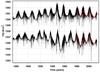 |
Fig. A.1 Hindcasting based on unrestricted multicomponent models. Using PSI to PMOD mapping (upper curve), PSI to ACRIM (lower curve, shifted down by five units). In red we plot the low-frequency backbones of the target curves. The cross correlation between the two curves is only Rc = 0.512 (see Fig. 10b). |
Appendix B: Mutual correlations of the computed hindcasts for all proxy-target pairs
The different solutions for the hindcasting problem can be compared by computing their correlations for the time intervals they share. There are 36 different correlation values for both prediction methods (simplest and restricted multicomponent models). We present the full list of correlations in Tables B.1 (simplest) and B.2 (multicomponent). Some solutions correlate at a very high level. For instance, the PSI to PMOD and PSI to RMIB predictions that are computed using the simple method correlate at the level of 0.9997. The worst case is between the SN to PMOD and SA to ACRIM predictions that are computed using multicomponent method (Rc = 0.8041). Here the scatter between different solutions is a result of many contributing factors: differences between PMOD and ACRIM (the main hindrance for better hindcasting), information content difference between proxies (SN against SA), and inherent modeling errors of the method. These tables clearly show that the correlations on the diagonals of the subtables are more narrowly spread than the overall scatter (these are the pairs with common proxies). For the simple method, the spread on diagonals is 0.9957−0.9997, and for the full scale method it is 0.8879−0.9836.
Correlations between proxy-target combinations for the simplest model.
Correlations between proxy-target combinations for the multicomponent model.
All Tables
Regression model in standard format for the PMOD target built using PSI as a proxy.
Prediction vs. target correlations for the simplest regression model and for the BvM variant of it.
Modeling PMOD data using PSI as a proxy. Regression components and iteration progress.
Modeling ACRIM data using PSI as a proxy. Regression components and iteration progress.
All Figures
|
Fig. 1 Three different transmission curves for a specific width of the time domain filter. |
| In the text | |
|
Fig. 2 Two different transmission curves for bandpass filters. |
| In the text | |
|
Fig. 3 Fragment of bandpass filtered PSI data set E [W,O] (t) with upper E+ [W,O] (t) and lower E− [W,O] [t] envelopes. The envelopes are much smoother and have a sidedness that can take correlations or anticorrelations into account. |
| In the text | |
|
Fig. 4 Fragment of bandpass-filtered PSI data set E [W,O] (t) (thin curve above), its upper envelope E+ [W,O] (t) (thick curve), and the corresponding detrended version |
| In the text | |
|
Fig. 5 Main controversy. To recover TSI for the past dates, we need reliable current estimates for calibration. The LF parts (obtained with a Gaussian smoothing filter with W0 = 750) of three target TSI composites differ significantly, however. The curves are shifted to a common level at 1996.465. |
| In the text | |
|
Fig. 6 Scatter plots for PSI-PMOD pair: a) – linear fit of the proxy to data (Rc = 0.020); b) – regression modeling using the simple model (Rc = 0.860); c) – multicomponent model (Rc = 0.893). |
| In the text | |
|
Fig. 7 FDCs between overlapping parts of the PMOD and PSI data sets as function of the band-pass offset Δν. Width |
| In the text | |
|
Fig. 8 Fragment of the simplest prediction from PSI to PMOD together with the BvM version and the target PMOD data. |
| In the text | |
|
Fig. 9 LF parts of the simplest prediction using PSI as the proxy and PMOD as the target. |
| In the text | |
|
Fig. 10 Correlations between PMOD and ACRIM and regression models based on them (using PSI as the proxy): a) cross plot of the original target data sets PMOD vs. ACRIM (Rc = 0.861); b) cross plot for the solution without restrictions (Rc = 0.512, Fig. A.1, see Appendix A.); c) cross plot based on the simplest models (Rc = 0.998); d) cross plot between restricted multicomponent models (Rc = 0.941). |
| In the text | |
|
Fig. 11 Hindcasting based on multicomponent models. PSI to PMOD mapping (upper curve) and PSI to ACRIM (shifted down by five units; lower curve). In red we plot the low-frequency backbones of the target curves. The cross correlation between the two hindcast curves is Rc = 0.941 (see Fig. 10d). |
| In the text | |
|
Fig. 12 Prediction errors (absolute differences) between predicted curves and targets for the PSI to PMOD pair (upper panel) and corresponding BvM solution (lower panel). Black shows the daily errors, red the errors for filter curves smoothed by W = 30, and green the errors for filter curves smoothed by W = 365 . The data sets are nearly 14 000 points long, and consequently, the plot points essentially mark the local maxima of the curves (for each pixel). The scatter of the errors can also be characterized by their standard deviations: 0.169, 0.113, and 0.076 for the upper panel and 0.156, 0.090, and 0.025 for the lower panel. |
| In the text | |
|
Fig. A.1 Hindcasting based on unrestricted multicomponent models. Using PSI to PMOD mapping (upper curve), PSI to ACRIM (lower curve, shifted down by five units). In red we plot the low-frequency backbones of the target curves. The cross correlation between the two curves is only Rc = 0.512 (see Fig. 10b). |
| In the text | |
Current usage metrics show cumulative count of Article Views (full-text article views including HTML views, PDF and ePub downloads, according to the available data) and Abstracts Views on Vision4Press platform.
Data correspond to usage on the plateform after 2015. The current usage metrics is available 48-96 hours after online publication and is updated daily on week days.
Initial download of the metrics may take a while.