| Issue |
A&A
Volume 599, March 2017
|
|
|---|---|---|
| Article Number | L2 | |
| Number of page(s) | 4 | |
| Section | Letters | |
| DOI | https://doi.org/10.1051/0004-6361/201630123 | |
| Published online | 22 February 2017 | |
Dependence of sunspot photospheric waves on the depth of the source of solar p-modes
1 Instituto de Astrofísica de Canarias, C/ vía Láctea, s/n, 38205 La Laguna, Tenerife, Spain
e-mail: tobias@iac.es
2 Departamento de Astrofísica, Universidad de La Laguna, 38205 La Laguna, Tenerife, Spain
Received: 23 November 2016
Accepted: 3 February 2017
Photospheric waves in sunspots moving radially outward at speeds faster than the characteristic wave velocities have been recently detected. It has been suggested that they are the visual pattern of p-modes excited around 5 Mm beneath the sunspot’s surface. Using numerical simulations, we performed a parametric study of the waves observed at the photosphere and higher layers that were produced by sources located at different depths beneath the sunspot’s surface. The observational measurements are consistent with waves driven between approximately 1 Mm and 5 Mm below the sunspot’s surface.
Key words: methods: numerical / Sun: oscillations / Sun: helioseismology / sunspots / Sun: photosphere
© ESO, 2017
1. Introduction
Sunspots’ atmospheres exhibit a wide variety of oscillatory phenomena. Their photosphere is dominated by five-minute oscillations (Thomas et al. 1982), whereas at the chromosphere three-minutes oscillations become stronger. These chromospheric waves have been identified as upward-propagating, field-aligned, slow-mode waves (Centeno et al. 2006; Bloomfield et al. 2007; Felipe et al. 2010b) that can develop into shocks and lead to the appearance of umbral flashes (Rouppe van der Voort et al. 2003; de la Cruz Rodríguez et al. 2013). Umbral flashes were first detected as sudden brightness increases in the core of Ca ii lines (Beckers & Tallant 1969). They are found to be related to running penumbral waves (RPWs Zirin & Stein 1972; Giovanelli 1972), which are observed as disturbances propagating radially outward at the chromospheric penumbra. The origin of RPWs has been a matter of debate over the years. It is currently acknowledged that they are the visual pattern of slow low-β plasma waves propagating up from the photosphere along the inclined magnetic field lines (Bloomfield et al. 2007; Jess et al. 2013; Madsen et al. 2015). According to the current understanding, all sunspot waves are different manifestations of a common process of magnetoacoustic wave propagation (Khomenko & Collados 2015).
This picture has recently been reinforced by the report of the photospheric counterpart of RPWs (Löhner-Böttcher & Bello González 2015). It was observed that, due to the variation of the inclination of the penumbral magnetic field with height, the apparent horizontal velocity of the RPWs decreases from the photosphere to the chromosphere. In addition to this direct observation, a similar photospheric wave was detected using helioseismic techniques (Zhao et al. 2015). The phase velocity of this wave (around 45 km s-1) was found to be faster than that of the MHD waves at the photosphere. It has been proposed that this fast-moving wave corresponds to the visual pattern of p-modes driven beneath the sunspot.
In this Letter, we aim to explore the nature of RPWs by analyzing numerical simulations of wave propagation in sunspots excited by sources at different depths. Under the assumption that the photospheric RPWs and the fast-moving waves are the same phenomenon, we indistinctly use both terms in order to refer to these waves. We describe the methods used for the development of the numerical simulations in Sect. 2, the results are presented in Sect. 3, and the conclusions are discussed in Sect. 4.
2. Numerical simulations
We used the code MANCHA (Khomenko & Collados 2006; Felipe et al. 2010a) for solving the ideal MHD equations for perturbations. These are obtained after explicitly removing the equilibrium state from the continuity, momentum, internal energy, and induction equations. The numerical simulations were restricted to the linear regime by choosing a small amplitude for the driver. Periodic boundary conditions were imposed at the horizontal directions. Perfect matched layers (Berenger 1996) were used to avoid wave reflection at the top and bottom boundaries.
Simulations were computed under the 2.5D approximation. This means that vectors keep their three components but the derivatives in the Y direction have been neglected. Photospheric RPWs have been reported in actual observations using time-slice analyses in the radial direction of the sunspot (Löhner-Böttcher & Bello González 2015) or using azimuthal averaged time-distance diagrams (Zhao et al. 2015). In both cases, a two-dimensional computation domain crossing the center of the sunspot is sufficient to compare the numerical results with the observations. The Alfvén speed was limited to a maximum value of 1000 km s-1 by modifying the Lorentz force following Rempel et al. (2009). According to Moradi & Cally (2014), this limiter can affect the results if the maximum allowed Alfvén speed is not sufficiently higher than the horizontal phase speeds of interest. Our chosen value is well above the phase velocities under study.
Our sunspot model was constructed following Khomenko & Collados (2008). The procedures were modified to extend the atmosphere up to the corona. This method requires the selection of the stratification at the sunspot axis and at a quiet Sun region as boundary conditions. For the photospheric and chromospheric layers, we chose VAL-C model (Vernazza et al. 1981) for the quiet Sun, and the semi-empirical model of Avrett (1981) for the sunspot umbra. For both models, the interior was taken from the convectively stabilized CSM_B model (Schunker et al. 2011) and an isothermal corona with a temperature of one million Kelvin was added following Santamaria et al. (2015). The photospheric magnetic field at the umbra was set at 900 G and the Wilson depression was set to 450 km. The field strength is significantly lower than that expected in large sunspots, but the model qualitatively reproduces properties of wave propagation through magnetic structures. The computational domain spanned from z = −7.30 Mmto z = 10.65 Mmand it was sampled by 360 equally spaced points in the vertical direction (vertical sampling of 50 km). The vertical position z = 0 was located at the umbral height where the optical depth at 500 nm (τ) is unity. The horizontal domain covered 120 Mmwith a spatial sampling of 150 km. The axis of the sunspot was located at the center of the domain.
The wave field was driven by spatially-localized sources of the vertical force added to the equations. The shape and temporal variation of each source is described by Parchevsky et al. (2008). This driver generates a wave field that resembles the solar spectrum (e.g., Parchevsky et al. 2008; Felipe et al. 2016). We performed several independent numerical experiments that differed in the amount and location of the sources. In the first set of simulations, we computed six simulations containing one single source located at the axis of the sunspot, but at different depths between z = −5.3 Mm and z = −0.3 Mm with 1 Mm intervals. The sources were placed beneath the sunspot following the suggestion of Zhao et al. (2015). In the second set of simulations, we reproduced the stochastic solar wave field by introducing a new source every 0.5 s at a randomly chosen horizontal location, but for each run the depth of the sources were fixed to the same geometrical depths used for the single source simulations. Each of the sources has the same frequency spectrum used for the single source cases, with a central frequency at 3.3 mHz.
3. Results
Maps of vertical velocity at constant optical depth were constructed by interpolating the vertical variation of the z velocity to the height where log τ takes the chosen value, at each horizontal position and time step. For most of the analyses in this Letter, we focus on the maps at log τ = −2, which provides a good characterization of the formation height of the Fe i 630.15 nm line that was used for the detection of RPWs in actual observations.
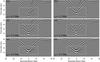 |
Fig. 1 Time-distance diagrams at log τ = −2 for the simulations containing waves driven by a single source located at the center of the sunspot. Each panel corresponds to a different source depth: zs = −0.3 Mm (a), zs = −1.3 Mm (b), zs = −2.3 Mm (c), zs = −3.3 Mm (d), zs = −4.3 Mm (e), and zs = −5.3 Mm (f). Color lines illustrate the track of the fast-moving waves. Dotted lines in the top right part of all panels show a linear fit of the reflected fast wave. Dashed lines in panels a)−c) show a linear fit of the helioseismic waves. Dashed white boxes delimit the first wavefronts of the fast-moving wave. |
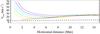 |
Fig. 2 Phase velocity of the fast-moving waves produced by a single source at zs = −0.3 Mm (red), zs = −1.3 Mm (yellow), zs = −2.3 Mm (green), zs = −3.3 Mm (light blue), zs = −4.3 Mm (dark blue), and zs = −5.3 Mm (violet). The dashed line shows the fast-wave speed at log τ = −2. |
3.1. Single source
Figure 1 shows the time-distance diagrams of the simulations with one isolated source located at the center of the sunspot at different depths. In all cases the white dashed boxes delimit the first wavefronts of a wave that sweeps outward with a speed higher than the local fast magnetoacoustic speed (around 10 km s-1). These fast-moving waves are produced because the wavefronts driven in the interior of the Sun take different times to reach the photosphere at different horizontal positions. The sources mainly generate fast high-β plasma acoustic waves with approximately spherical wavefronts. In the interior, they propagate in all directions at the local sound speed. The region of the wavefront above the source is the first one to become visible at the photosphere. It is then followed by the surrounding parts of the wavefront. As the wavefronts reach the photosphere at progressively farther horizontal locations, an apparent radially-propagating wave appears at log τ = −2.
The color lines in Fig. 1 illustrate the position of the wavefront of the fast-moving wave. The phase velocity of this apparent wave is given in Fig. 2. When the first appearance of the wave is produced, the wavefront propagating upward is nearly parallel to the log τ = −2 surface. The initial velocity of the fast-moving wave is very high because regions of the wavefront at a certain horizontal distance reach the photosphere almost simultaneously. For deeper sources, the wavefront of the incident wave is flatter and, thus, the fast-moving wave initially shows a higher apparent velocity. The apparent velocity is reduced with distance. At horizontal distances around 12 Mmfrom the origin, the velocity of the fast-moving waves is around 25 km s-1for all the simulations with different source depths. The dashed line in Fig. 2 indicates the velocity of the fast wave at the surface log τ = −2. It is between 7 and 10 km s-1for all horizontal locations, which is clearly slower than the phase velocity of the apparent wave. The fast-wave speed for a sunspot model with a more realistic photospheric magnetic field strength, around 3000 G, is below 15 km s-1and thus still lower than the measured phase velocity.
Other wave branches are present in our simulations. The three simulations with the shallower sources (panels a−c from Fig. 1) show the usual helioseismic waves after about 23 min of simulation. In each of these panels, one of those wavefronts is indicated by a dashed line obtained from a linear fit. In these three cases these wavefronts correspond to a phase velocity of 10 km s-1and are thus in agreement with the local fast velocity. The helioseismic wave is barely visible in the cases with the source located at depths below z = −2.3 Mm.
Another distinct branch with much higher phase velocity is found at longer radial distances in all simulations. It appears around 10 min after the first velocity perturbations are visible but it is more easily seen at later time steps. We refer to these as super-fast-moving waves. One of those wavefronts is marked in all panels of Fig. 1 by a dotted line. The phase velocity of super-fast moving waves is between 222 and 277 km s-1. A careful inspection of the temporal evolution of the simulations reveals that these waves are the visual pattern of the fast magnetic wave coming after reflection from the upper part of the atmosphere. The source (located in the interior in a high-β region) drives fast acoustic waves which reach the photosphere. At the surface β ~ 1 they are converted into fast magnetic and slow acoustic waves (low-β region). The fast magnetic waves are refracted due to the gradients of the Alfvén speed (Rosenthal et al. 2002; Khomenko & Collados 2006) and they return toward the interior of the Sun. In our simulations, fast waves are detected up to the high-chromosphere where only almost-vertical fast waves can penetrate. Waves with higher inclinations are reflected at lower heights around the mid-chromosphere. Their wavefronts form a certain angle with respect to the surface log τ = −2, and the sections closer to the umbra reach the photosphere earlier than the sections at longer radial distances. They appear as an apparent wave propagating radially outward. This effect is similar to that producing the fast-moving wave, but the latter is generated by p-modes coming from the interior whereas the former is due to the return of atmospheric waves. Independent simulations (not shown in the figures) with the same configuration but with the magnetic field set to zero were computed. In this case the super-fast-moving waves do not appear, confirming that their presence is associated with mode conversion. Because the Lorentz force was limited to a maximum value of the Alfvén speed of 1000 km s-1, these simulations do not capture all the physics of the fast wave refraction. However, we expect that the results found in our simulations qualitatively match the unrestricted process.
3.2. Stochastic sources
The cross-correlation of the oscillatory signal measured at one location with those observed at other locations is a common helioseismic approach for the analysis and interpretation of stochastic wave-fields (e.g., Duvall et al. 1993; Cameron et al. 2008; Zhao et al. 2011). For each map at log τ, we cross-correlated the vertical velocity signal at xref = 7.5 Mmwith the vertical velocity at all other locations inside the area of interest. The location xref corresponds to the penumbra at approximately the same radial distance where the RPWs were reported by Löhner-Böttcher & Bello González (2015). The cross-correlation at time lag t indicates the position of a wave packet at time t after (before) it has left (arrived) from (at) xref.
The cross-correlations of maps at various heights arising from different optical depths (between the base of the photosphere and the low chromosphere) reveals that the apparent velocity of the wave moving radially outward monotonically decreases with height. The variation of the velocity with height shows a similar trend for all the simulations, independently of the depth of the sources. This reduction of the apparent horizontal velocity of RPWs from the photosphere to the chromosphere is in agreement with the recent observations from Löhner-Böttcher & Bello González (2015).
We found that the phase velocity of the wave detected in the cross-correlation does depend on the depth of the stochastic sources. Figure 3 illustrates the time-distance diagrams at log τ = −2 for all the simulations. For the cases with zs = −1.3 Mmand deeper, the cross-correlation clearly isolates the wavefront of a wave moving from the inner to the outer penumbra. In the case of the simulation with the sources at zs = −0.3 Mm, high correlation and anti-correlation is found for several wavefronts, but the radially outward movement is also prominent. Deeper sources lead to faster horizontal velocities, similar to our results for the single source simulations. A maximum horizontal velocity at log τ = −2 of 71 km s-1is obtained when the sources are located at zs = −5.3 Mm, whereas shallow sources at zs = −0.3 Mmproduce a horizontal velocity of 17 km s-1. The cross-correlation of an independent simulation with no sources located beneath the sunspot within radial distances of 10 Mm shows a radially-inward-propagating wave, excited by the sources located outside of the spot.
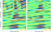 |
Fig. 3 Time-distance diagrams at log τ = −2 for the simulations containing stochastic drivers obtained from the cross-correlation between the vertical velocity at x = 7.5 Mmand the vertical velocity at the x positions indicated in the horizontal axis. Each panel corresponds to a different source depth: zs = −0.3 Mm (a), zs = −1.3 Mm (b), zs = −2.3 Mm (c), zs = −3.3 Mm (d), zs = −4.3 Mm (e), and zs = −5.3 Mm (f). |
4. Discussion and conclusions
Löhner-Böttcher & Bello González (2015) recently reported the observation of RPWs at photospheric layers. They present apparent horizontal velocities of 51 ± 13 km s-1, which decrease to 37 ± 10 km s-1at the chromosphere. A similar photospheric wave was independently detected through helioseismic analyses by Zhao et al. (2015). Because the apparent speed of the wave is faster than magnetoacoustic or Alfvén waves speed at the photosphere of sunspots, Zhao et al. (2015) proposed that the observed waves are the visual pattern of acoustic waves driven about 5 Mm beneath sunspot’s surface, whose wavefronts sweep across the photosphere.
Motivated by this hypothesis, we performed a parametric study of the dependence of the visible waves at the photosphere and higher layers upon the depth of the sources driving them. Twelve numerical simulations were developed, six of them with a single source and the other six with stochastic sources. In both sets of simulations the drivers were located at different depths between −5.3 and −0.3 Mm. The results show a prominent wave propagating radially outward at a faster velocity than that of the MHD waves at the photosphere of sunspots. This fast-moving wave is produced by the p-modes generated in the interior by the sources, whose almost spherical wavefronts expand and reach the surface at different times at each horizontal location. A simulation similar to those with a single source has recently proved that this model qualitatively resembles the observed properties and the shape of the atmospheric wavefronts (from the photosphere to the corona) retrieved from a helioseismic analysis (Zhao et al. 2016).
Convective motions near the surface of the Sun are known to be the source of excitation of the p-modes. Many works have attempted to infer the properties of these sources from the analysis of velocity and intensity power-spectra asymmetries (e.g., Roxburgh & Vorontsov 1997; Chaplin & Appourchaux 1999; Kumar & Basu 1999; Nigam & Kosovichev 1999). The depth of the sources obtained from these analyses is highly sensitive to the model selection, and these works have provided estimates of between 75 and 1500 km beneath the photosphere. In addition, more recent works have found that the acoustic source depth cannot be uniquely determined from the properties of the resonant p-modes (Jefferies et al. 2003; Wachter & Kosovichev 2005). From a comparison between the observed photospheric RPWs’ velocities and the source-depth dependence of their apparent wave velocities in the simulations, we can estimate the location of the sources in sunspots. The velocity of the fast-moving wave obtained from the cross-correlation of the simulations with stochastic sources is within the limits of the speed of the photospheric RPWs measured by Löhner-Böttcher & Bello González (2015) for source depths between zs = −1.3 Mmand zs = −4.3 Mm. As reported by Zhao et al. (2015), the fast-moving wave only appears in sunspots. Our results suggest that in sunspots, the source of excitation of p-modes is extended to deeper regions up to almost 5 Mm beneath the surface.
The propagation velocity of the fast-moving wave strongly depends on the distance from the horizontal position of the source, as seen in Fig. 2. When this distance is shorter, the apparent velocity is maximal and it increases with the depth of the source. At larger horizontal distances all the source depths produce similar apparent velocities. The velocities of the fast-moving waves measured from the cross-correlation in the stochastic simulations are in good agreement with those obtained from measurements taken at short horizontal distances from single sources confirming that the wave detected using helioseismic method corresponds to the same fast-moving wave identified in the single source simulations. Our simulations also show that sources deeper than zs = −2.3 Mm are not efficient at driving the usual helioseismic waves. Only the simulations with shallower sources lead to the appearance of waves propagating at the fast magnetoacoustic speed (panels a, b, and c from Fig. 1).
The simulations show another wave that we have called super-fast-moving wave. This is also an apparent wave but is produced by the fast magnetic waves which are refracted at atmospheric layers. The study of this wave can potentially provide some insights about the magnetic field in the solar atmosphere, although its detection can be challenging due to its low amplitude in comparison with the photospheric RPWs and the p-modes, and its fast apparent speed.
Acknowledgments
We acknowledge financial support from the Spanish Ministry of Economy and Competitiveness (MINECO) through projects AYA2014-55078-P, AYA2014-60476-P, and AYA2014-60833-P. This work used the Teide High Performance Computing facilities at Instituto Tecnológico y de Energías Renovables (ITER, SA) and the MareNostrum supercomputer at Barcelona Supercomputing Center.
References
- Avrett, E. H. 1981, in The Physics of Sunspots, eds. L. E. Cram, & J. H. Thomas, 235 [Google Scholar]
- Beckers, J. M., & Tallant, P. E. 1969, Sol. Phys., 7, 351 [NASA ADS] [CrossRef] [MathSciNet] [Google Scholar]
- Berenger, J. P. 1996, J. Comput. Phys., 127, 363 [NASA ADS] [CrossRef] [Google Scholar]
- Bloomfield, D. S., Solanki, S. K., Lagg, A., Borrero, J. M., & Cally, P. S. 2007, A&A, 469, 1155 [NASA ADS] [CrossRef] [EDP Sciences] [Google Scholar]
- Cameron, R., Gizon, L., & Duvall, Jr., T. L. 2008, Sol. Phys., 251, 291 [NASA ADS] [CrossRef] [Google Scholar]
- Centeno, R., Collados, M., & Trujillo Bueno, J. 2006, ApJ, 640, 1153 [NASA ADS] [CrossRef] [PubMed] [Google Scholar]
- Chaplin, W. J., & Appourchaux, T. 1999, MNRAS, 309, 761 [NASA ADS] [CrossRef] [Google Scholar]
- de la Cruz Rodríguez, J., Rouppe van der Voort, L., Socas-Navarro, H., & van Noort, M. 2013, A&A, 556, A115 [NASA ADS] [CrossRef] [EDP Sciences] [Google Scholar]
- Duvall, Jr., T. L., Jefferies, S. M., Harvey, J. W., & Pomerantz, M. A. 1993, Nature, 362, 430 [NASA ADS] [CrossRef] [Google Scholar]
- Felipe, T., Khomenko, E., & Collados, M. 2010a, ApJ, 719, 357 [Google Scholar]
- Felipe, T., Khomenko, E., Collados, M., & Beck, C. 2010b, ApJ, 722, 131 [NASA ADS] [CrossRef] [Google Scholar]
- Felipe, T., Braun, D. C., Crouch, A. D., & Birch, A. C. 2016, ApJ, 829, 67 [NASA ADS] [CrossRef] [Google Scholar]
- Giovanelli, R. G. 1972, Sol. Phys., 27, 71 [NASA ADS] [CrossRef] [Google Scholar]
- Jefferies, S. M., Severino, G., Moretti, P.-F., Oliviero, M., & Giebink, C. 2003, ApJ, 596, L117 [Google Scholar]
- Jess, D. B., Reznikova, V. E., Van Doorsselaere, T., Keys, P. H., & Mackay, D. H. 2013, ApJ, 779, 168 [NASA ADS] [CrossRef] [Google Scholar]
- Khomenko, E., & Collados, M. 2006, ApJ, 653, 739 [Google Scholar]
- Khomenko, E., & Collados, M. 2008, ApJ, 689, 1379 [NASA ADS] [CrossRef] [Google Scholar]
- Khomenko, E., & Collados, M. 2015, Liv. Rev. Sol. Phys., 12, 6 [CrossRef] [Google Scholar]
- Kumar, P., & Basu, S. 1999, ApJ, 519, 396 [NASA ADS] [CrossRef] [Google Scholar]
- Löhner-Böttcher, J., & Bello González, N. 2015, A&A, 580, A53 [NASA ADS] [CrossRef] [EDP Sciences] [Google Scholar]
- Madsen, C. A., Tian, H., & DeLuca, E. E. 2015, ApJ, 800, 129 [NASA ADS] [CrossRef] [Google Scholar]
- Moradi, H., & Cally, P. S. 2014, ApJ, 782, L26 [NASA ADS] [CrossRef] [Google Scholar]
- Nigam, R., & Kosovichev, A. G. 1999, ApJ, 514, L53 [NASA ADS] [CrossRef] [Google Scholar]
- Parchevsky, K. V., Zhao, J., & Kosovichev, A. G. 2008, ApJ, 678, 1498 [NASA ADS] [CrossRef] [Google Scholar]
- Rempel, M., Schüssler, M., & Knölker, M. 2009, ApJ, 691, 640 [NASA ADS] [CrossRef] [Google Scholar]
- Rosenthal, C. S., Bogdan, T. J., Carlsson, M., et al. 2002, ApJ, 564, 508 [NASA ADS] [CrossRef] [Google Scholar]
- Rouppe van der Voort, L. H. M., Rutten, R. J., Sütterlin, P., Sloover, P. J., & Krijger, J. M. 2003, A&A, 403, 277 [NASA ADS] [CrossRef] [EDP Sciences] [Google Scholar]
- Roxburgh, I. W., & Vorontsov, S. V. 1997, MNRAS, 292, L33 [NASA ADS] [Google Scholar]
- Santamaria, I. C., Khomenko, E., & Collados, M. 2015, A&A, 577, A70 [NASA ADS] [CrossRef] [EDP Sciences] [Google Scholar]
- Schunker, H., Cameron, R. H., Gizon, L., & Moradi, H. 2011, Sol. Phys., 271, 1 [NASA ADS] [CrossRef] [Google Scholar]
- Thomas, J. H., Cram, L. E., & Nye, A. H. 1982, Nature, 297, 485 [NASA ADS] [CrossRef] [Google Scholar]
- Vernazza, J. E., Avrett, E. H., & Loeser, R. 1981, ApJS, 45, 635 [NASA ADS] [CrossRef] [Google Scholar]
- Wachter, R., & Kosovichev, A. G. 2005, ApJ, 627, 550 [Google Scholar]
- Zhao, J., Kosovichev, A. G., & Ilonidis, S. 2011, Sol. Phys., 268, 429 [NASA ADS] [CrossRef] [Google Scholar]
- Zhao, J., Chen, R., Hartlep, T., & Kosovichev, A. G. 2015, ApJ, 809, L15 [NASA ADS] [CrossRef] [Google Scholar]
- Zhao, J., Felipe, T., Chen, R., & Khomenko, E. 2016, ApJ, 830, L17 [NASA ADS] [CrossRef] [Google Scholar]
- Zirin, H., & Stein, A. 1972, ApJ, 178, L85 [NASA ADS] [CrossRef] [Google Scholar]
All Figures
|
Fig. 1 Time-distance diagrams at log τ = −2 for the simulations containing waves driven by a single source located at the center of the sunspot. Each panel corresponds to a different source depth: zs = −0.3 Mm (a), zs = −1.3 Mm (b), zs = −2.3 Mm (c), zs = −3.3 Mm (d), zs = −4.3 Mm (e), and zs = −5.3 Mm (f). Color lines illustrate the track of the fast-moving waves. Dotted lines in the top right part of all panels show a linear fit of the reflected fast wave. Dashed lines in panels a)−c) show a linear fit of the helioseismic waves. Dashed white boxes delimit the first wavefronts of the fast-moving wave. |
| In the text | |
|
Fig. 2 Phase velocity of the fast-moving waves produced by a single source at zs = −0.3 Mm (red), zs = −1.3 Mm (yellow), zs = −2.3 Mm (green), zs = −3.3 Mm (light blue), zs = −4.3 Mm (dark blue), and zs = −5.3 Mm (violet). The dashed line shows the fast-wave speed at log τ = −2. |
| In the text | |
|
Fig. 3 Time-distance diagrams at log τ = −2 for the simulations containing stochastic drivers obtained from the cross-correlation between the vertical velocity at x = 7.5 Mmand the vertical velocity at the x positions indicated in the horizontal axis. Each panel corresponds to a different source depth: zs = −0.3 Mm (a), zs = −1.3 Mm (b), zs = −2.3 Mm (c), zs = −3.3 Mm (d), zs = −4.3 Mm (e), and zs = −5.3 Mm (f). |
| In the text | |
Current usage metrics show cumulative count of Article Views (full-text article views including HTML views, PDF and ePub downloads, according to the available data) and Abstracts Views on Vision4Press platform.
Data correspond to usage on the plateform after 2015. The current usage metrics is available 48-96 hours after online publication and is updated daily on week days.
Initial download of the metrics may take a while.