| Issue |
A&A
Volume 599, March 2017
|
|
|---|---|---|
| Article Number | A63 | |
| Number of page(s) | 9 | |
| Section | Interstellar and circumstellar matter | |
| DOI | https://doi.org/10.1051/0004-6361/201629901 | |
| Published online | 01 March 2017 | |
H12CN and H13CN excitation analysis in the circumstellar outflow of R Sculptoris⋆
Department of Earth and Space Sciences, Chalmers University of Technology, Onsala Space Observatory, 43992 Onsala, Sweden
e-mail: maryam.saberi@chalmers.se
Received: 14 October 2016
Accepted: 6 December 2016
Context. The 12CO/13CO isotopologue ratio in the circumstellar envelope (CSE) of asymptotic giant branch (AGB) stars has been extensively used as the tracer of the photospheric 12C/13C ratio. However, spatially-resolved ALMA observations of R Scl, a carbon rich AGB star, have shown that the 12CO/13CO ratio is not consistent over the entire CSE. Hence, it can not necessarily be used as a tracer of the 12C/13C ratio. The most likely hypothesis to explain the observed discrepancy between the 12CO/13CO and 12C/13C ratios is CO isotopologue selective photodissociation by UV radiation. Unlike the CO isotopologue ratio, the HCN isotopologue ratio is not affected by UV radiation. Therefore, HCN isotopologue ratios can be used as the tracer of the atomic C ratio in UV irradiated regions.
Aims. We aim to present ALMA observations of H13CN(4–3) and APEX observations of H12CN(2–1), H13CN(2–1, 3–2) towards R Scl. These new data, combined with previously published observations, are used to determine abundances, ratio, and the sizes of line-emitting regions of the aforementioned HCN isotopologues.
Methods. We have performed a detailed non-LTE excitation analysis of circumstellar H12CN(J = 1–0, 2–1, 3–2, 4–3) and H13CN(J = 2–1, 3–2, 4–3) line emission around R Scl using a radiative transfer code based on the accelerated lambda iteration (ALI) method. The spatial extent of the molecular distribution for both isotopologues is constrained based on the spatially resolved H13CN(4–3) ALMA observations.
Results. We find fractional abundances of H12CN/H2 = (5.0 ± 2.0) × 10-5 and H13CN/H2 = (1.9 ± 0.4) × 10-6 in the inner wind (r ≤ (2.0 ± 0.25) ×1015 cm) of R Scl. The derived circumstellar isotopologue ratio of H12CN/H13CN = 26.3 ± 11.9 is consistent with the photospheric ratio of 12C/13C ~ 19 ± 6.
Conclusions. We show that the circumstellar H12CN/H13CN ratio traces the photospheric 12C/13C ratio. Hence, contrary to the 12CO/13CO ratio, the H12CN/H13CN ratio is not affected by UV radiation. These results support the previously proposed explanation that CO isotopologue selective-shielding is the main factor responsible for the observed discrepancy between 12C/13C and 12CO/13CO ratios in the inner CSE of R Scl. This indicates that UV radiation impacts on the CO isotopologue ratio. This study shows how important is to have high-resolution data on molecular line brightness distribution in order to perform a proper radiative transfer modelling.
Key words: stars: abundances / stars: AGB and post-AGB / stars: individual: R Scl / binaries: general / circumstellar matter / stars: carbon
© ESO, 2017
1. Introduction
During late stellar evolutionary phases, stars produce almost all heavy elements in the universe through nucleosynthesis. In the last phase of evolution of low- and intermediate-mass stars (0.8−8 M⊙), heavy elements that are gradually built up in the inner layers are dredged up to the surface and are injected into the interstellar medium through intense stellar winds. These stars lose up to 80 percent of their initial mass typically at rates of 10-8−10-4M⊙ yr-1 during the asymptotic giant branch (AGB) phase. As a result, a circumstellar envelope (CSE) of gas and dust forms around the central star, (e.g. Habing 1996; Habing & Olofsson 2003). AGB stars can be classified by the elemental C/O ratio: C/O > 1 the carbon rich C-type stars, C/O ~ 1 the S-type stars and C/O < 1 the oxygen rich M-type stars.
Molecular emission lines from CSEs are excellent probes of the physical and chemical properties of the CSE and the central star. Observations of CO rotational transitions provide the most reliable measurements of the physical parameters of the CSE such as the mass-loss rate, density structure, expansion-velocity profile, kinetic temperature, and spatial extent (e.g. Neri et al. 1998; Schöier & Olofsson 2000; Ramstedt et al. 2008; Castro-Carrizo et al. 2010; De Beck et al. 2010). Observations of other abundant molecules set strong constraints on the chemical networks active in the CSE (e.g. Omont et al. 1993; Bujarrabal et al. 1994; Maercker et al. 2008, 2009; De Beck et al. 2012; Quintana-Lacaci et al. 2016).
The study of isotopic ratios of evolved stars provides important information on the stellar evolutionary phases and chemical enrichment of the interstellar medium. The photospheric 12C/13C ratio is a good tracer of the stellar nucleosynthesis. From an observational point of view, a direct estimate of the 12C/13C ratio is very challenging. Hence, observing isotopologues of circumstellar carbon-bearing molecules are widely used to trace the elemental isotopic carbon ratio. Carbon monoxide, as the most abundant C-bearing molecule, has been extensively used to extract the carbon isotope ratio (e.g. Groenewegen et al. 1996; Greaves & Holland 1997; Schöier & Olofsson 2000; Milam et al. 2009).
Assuming a solitary AGB star, known processes that may affect the chemical composition of the CSE are shocks due to stellar pulsations (e.g. Cherchneff 2012) and chromospheric activity in the inner wind (~ r< 2.5×1014 cm), gas-dust interaction in the intermediate wind (~ 2.5×10¹⁴<r< 5 × 1015 cm), and photodissociation by the interstellar UV-radiation, associated photo-induced chemistry, and chemical fractionation processes, in the outer wind (~ r> 5 × 1015 cm) (e.g. Decin et al. 2010). In the case of a clumpy envelope structure, the interstellar UV-radiation can penetrate the entire envelope and affect the chemistry in the inner wind (e.g. Agúndez et al. 2010).
The chemical processes in the inner and intermediate wind are not expected to affect the isotopologues abundance ratios. However, differences in self-shielding against UV-radiation do cause different photodissociation rates of molecules with sharp discrete absorption bands such as isotopologues of H2, CO, C2H2, NO, (Lee 1984). Thus, isotopologue selective photodissociation by UV radiation can change the isotopologue abundance ratios in the UV irradiated regions (e.g. Savage & Sembach 1996; Visser et al. 2009). Moreover, ion-molecule charge-exchange reactions in cold regions may also affect the isotopologue abundance ratios (e.g. Watson et al. 1976).
Photodissociation of the molecular gas in the CSEs is thought to be dominated by the interstellar radiation field (ISRF) from the outside. ISRF is the only UV radiation field which has been considered in the modelling of AGB CSEs. However, previous studies of UV spectra indicate the presence of a chromosphere in the outer atmosphere of carbon stars (Johnson et al. 1986; Eaton & Johnson 1988). In binary systems, active binary companions can emit UV-radiation from the inside as well (e.g. Sahai et al. 2008; Ortiz & Guerrero 2016). A recent search for UV emission from AGB stars has revealed that about 180 AGB stars, ~50% of the AGB stars observed with Galaxy Evolution Explorer (GALEX), have detectable near- or far-UV emission (Montez et al., in prep.), supporting the possible existence of internal sources of UV-radiation.
Nowadays, high spatial resolution Atacama Large Millimeter/submillimeter Array (ALMA) data enable us to study the impact of UV radiation sources on the isotopologue abundance ratios in the CSEs of evolved stars more accurately.
In this paper, we derive the H12CN/H13CN ratio and compare it with previously reported 12CO/13CO and 12C/13C ratios to probe the effect of UV radiation on the CSE of R Scl. We present the physical characteristics of R Scl in Sect. 2. New spectral line observations of R Scl are presented in Sect. 3. The excitation analysis of H12CN and H13CN is explained in Sect. 4. In Sect. 5, we present the results. Finally, we discuss our results and draw conclusion in Sects. 6 and 7, respectively.
2. R Sculptoris
R Scl is a carbon-type AGB star at a distance of approximately 370 pc derived using K-band period-luminosity relationships (Knapp et al. 2003; Whitelock et al. 2008). It is a semi-regular variable with a pulsation period of 370 days. The stellar velocity  =-19 km s-1 is determined from molecular line observations. A detached shell of gas and dust with a width of 2′′±1′′ was created during a recent thermal pulse at a distance of 19.5′′±0.5′′ from the central star (Maercker et al. 2012, 2014). This shell has been extensively observed in CO and dust scattered stellar light in the optical (e.g. González Delgado et al. 2001, 2003; Olofsson et al. 2010; Maercker et al. 2012, 2014). A spiral structure in the CSE of R Scl induced by a binary companion was revealed by 12CO(J = 3−2) ALMA observations (Maercker et al. 2012). Moreover, a recent study of the physical properties of the detached shell by Maercker et al. (2016b) show that the previously assumed detached shell around R Scl is filled with gas and dust.
High spatial resolution ALMA observations of 12CO and 13CO have allowed us to separate the detached-shell emission from the extended emission of the CSE (Maercker et al. 2012; Vlemmings et al. 2013). These observations reveal a discrepancy between the circumstellar 12CO/13CO and the photospheric 12C/13C ratios (Vlemmings et al. 2013, hereafter V13). They measure an intensity ratio of 12CO/13CO > 60 in the inner wind. Using detailed radiative transfer modelling, they show that this implies a carbon isotope ratio that is not consistent with the photospheric 12C/13C ~ 19 ± 6 reported by Lambert et al. (1986). At the same time, they measure the intensity ratio, which varies from 1.5 to 40 in the detached shell with the average intensity ratio of 12CO/13CO ~ 19 which, again taking into account radiative transfer, is still consistent with the photospheric 12C/13C ratio. Therefore, the circumstellar 12CO/13CO ratio from the inner parts of the CSE, provided by the high-resolution interferometric observations, does not necessarily measure the 12C/13C ratio. It has been suggested in V13 that the lack of 13CO in the recent mass loss might be due to the extra photodissociation of 13CO by internal UV radiation from the binary companion or chromospheric activity, while the more abundant 12CO would be self-shielded.
To confirm isotopologue selective photodissociation of CO as the reason for the observed discrepancy between the aforementioned CO isotopologue and C isotope ratios in R Scl, we compare the H12CN/H13CN and 12C/13C ratios. Both CO and HCN have line and continuum absorption bands in UV, respectively. Thus, CO isotopologues are photodissociated in well-defined bands, while HCN isotopologues are photodissociated via continuum. This implies that both HCN isotopologues would be equally affected by the UV-radiation, whereas CO isotopologues have different rates of photodissociation because of isotopologue self-shielding. Hence, this comparison would confirm the selective photodissociation of CO as the main reason for changing the CO isotopologue abundance ratio through the CSE of R Scl.
3. Observations
3.1. Single-dish data
Single-dish observations of H12CN(J = 2−1) and H13CN(J = 2−1, 3−2) emission lines towards R Scl were performed using the APEX 12 m telescope, located on Llano Chajnantor in northern Chile, in July 2015. We used the SEPIA/band 5 and the SHeFI-APEX1 receivers. The observations were made in a beam switching mode. The antenna main-beam efficiency, ηmb, the full-width half-power beam width, θmb, and the excitation energy of the upper transition level, Eup, at the observational frequencies for H12CN and H13CN are presented in Table 1.
The data reduction was done using XS1. A first-order polynomial was subtracted from the spectrum to remove the baseline. The measured antenna temperature was converted to the main-beam temperature using  .
.
In addition to the new data presented here, we have also used previously published single-dish observations of H12CN(J = 1−0, 3−2) made with the Swedish-ESO Submillimetre Telescope (SEST; Olofsson et al. 1996) and H12CN(J = 4−3) observed with the Heinrich Hertz Submillimeter Telescope (HHT; Bieging 2001), which are summarised in Table 1.
3.2. Interferometer data
The ALMA observations of H13CN(J = 4−3) were made on 14 Dec. 2013, 25 Dec., 26 Apr. 2014, and 24 Jul. 2015 using ALMA band 7 (275−373 GHz). Figure 1 shows the H13CN(J = 4−3) integrated flux density over the velocity channels, a zero-moment map. The primary flux calibration was done using Uranus and bootstrapped to the gain calibrator J0143-3206 (0.27 Jy beam-1) and J0106-4034 (0.23 Jy beam-1). Based on the calibrator fluxes, the absolute flux has an uncertainty of around 10%. The data reduction was done with the Common Astronomy Software Application (CASA). More details of the data reduction will come in Maercker et al., in prep. The tasks “imsmooth” and “immoments” in CASA were used to smooth the image to 0.13′′ × 0.13′′ resolution and to integrate over velocity channels, respectively.
Observations of HCN towards the circumstellar envelope of R scl.
4. Excitation analysis
4.1. Spectroscopic treatment of HCN
The molecule HCN is linear and polyatomic, with three vibrational modes: the H-C stretching mode ν1 at 3 μm, the bending mode ν2 at 14 μm, and the C-N stretching mode ν3 at 5 μm. In our modelling, we take into account the ν1 = 1 and the ν2 = 1 states, while we neglect the ν3 mode since this includes transitions that are about 300 times weaker than ν1 = 1 (Bieging et al. 1984). The nuclear spin (or electric quadrupole moment) of the nitrogen nucleus leads to a splitting of the rotational levels into three hyperfine components. Furthermore, a splitting of the bending mode occurs due to rotation when the molecule is bending and rotating simultaneously. This is referred to as l-type doubling. This interaction between the rotational and bending angular momenta results in l-doubling of the bending mode into two levels 011c0 and 011d0.
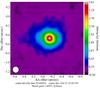 |
Fig. 1 Zero-moment H13CN(4–3) map of R Scl observed with ALMA. The ALMA beam size is shown in the bottom left corner. |
In our modelling, the excitation analysis includes 126 energy levels. Hyperfine splitting of the rotational levels for J = 1 levels are included. In each of the vibrational levels, rotational levels up to J = 29 are considered, and the l-type doubling for ν2 = 1 transitions are also included. For excitation analysis, the same treatment as Schöier et al. (2011), Danilovich et al. (2014) with small adjustments was used.
The HCN vibrational states are mainly radiatively excited (e.g. Lindqvist et al. 2000; Schöier et al. 2013). In our modelling, the radiation arises from the central star, which is assumed to be a black body, and from the dust grains, which are distributed through the CSE.
4.2. Radiative transfer model
To determine the HCN isotopologue abundances and constrain their distributions in the CSE, a non-local thermodynamic equilibrium (LTE) radiative transfer code based on the accelerated lambda iteration (ALI) method was used. The ALI method is described in detail by Rybicki & Hummer (1991). The code has been implemented by Maercker et al. (2008) and was previously used by Maercker et al. (2009) and Danilovich et al. (2014).
The CSE around R Scl is assumed to be spherically symmetric and is formed due to a constant mass loss rate Ṁ ~ 2×10⁻⁷M⊙ yr-1 (Wong et al. 2004, hereafter W04). The inner radius is assumed to be located at rin = 1014 cm. The H2 number density is calculated assuming a constant mass loss rate, as in Schöier & Olofsson (2001).
The gas-expansion profiles is assumed to be: 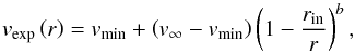 (1)where v∞ is the terminal expansion velocity and vmin is the minimum velocity at rin, which is taken as the sound speed 3 km s-1 and b determines the shape of the radial velocity profile. A detailed discussion on the determination of the two free parameters v∞ and b based on the shape of line profiles at radial offset positions from the ALMA observations is presented in Sect. 5.1.
The radial distribution of the dust temperature is derived based on SED modelling (Maercker, priv. comm.) to be a power-law given by: 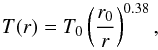 (2)where T0 = 1500 K and r0 = 7 × 1013 cm are the dust condensation temperature and radius. Since ALI does not solve the energy balance equation, the same temperature profile as the dust temperature was used to describe the kinetic temperature of the gas. We also ran models using the gas temperature profile derived by W04, which led to no significant change in the results.
The HCN fractional molecular abundance relative to H2(nHCN/nH2) is assumed to have a gaussian distribution: 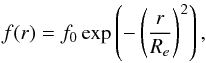 (3)where f0 denotes the initial fractional abundance and Re is the e-folding radius for HCN, the radius at which the abundance has dropped to 1/e (37%). The stellar parameters are presented in Table 2.
Stellar parameters used in the radiative transfer modelling of the H12CN and H13CN isotopologues around R Scl.
5. Results
5.1. Radial expansion velocity profile
We use the spatially resolved ALMA observations of H13CN(4−3) to constrain two free parameters, b and v∞, in the gas radial expansion velocity profile, Eq. (1). We extracted intensities at a series of offset positions sampling every independent beam from the ALMA observations and the corresponding intensities from the modelling results. A series of models with b and v∞ changing in the ranges 0.4 <b< 8.5 and 8.5 <v∞< 13 were run to get good fits to the line shape of spectra at all positions. The model with b = 2.5 and v∞ = 10 km s-1 leads to the best fits to the line shape of the H13CN(4−3) spectra at the offset positions from the centre. The velocity profiles with b = 0.4, 2.5 and 8.5 values are shown in Fig. 2. Models with b < 2.5 did not reproduce the shape of H13CN(4−3) line profiles in the inner part of the envelope (r 0.2′′); they predicted double-peaked line profiles contrary to the observed spectra. On the other hand, models with large b values reproduce narrow line shapes, which are also not consistent with the observations. To illustrate this, we plot the H13CN(4−3) intensity profiles at the centre of the star from ALMA observations and from three models with b = 0.4, 2.5 and 8.5 in Fig. 3. There is red-shifted excess emission in the ALMA H13CN(4−3) that can not be reproduced by our spherically symmetric model. The models with b = 0.4 and 8.5 can predict the total intensity of the H13CN(4−3) pretty well, but they fail to reproduce the line shapes at the inner part of the envelope (r 0.2′′). Without having spatially resolved observations, it is not possible to find out such effects and precisely constrain the gas expansion velocity profile.
It should be noted that the wind-expansion velocity of R Scl likely changes over time (Maercker et al. 2016b). The gas expansion velocity profile used here hence mostly describes the change in terminal expansion velocity, rather than the acceleration due to radiation pressure on dust grains. Typical values for the exponent in accelerated-wind profiles are approx. 1.5 for M-type stars (e.g. Maercker et al. 2016a) and even less for carbon stars. The fact that we derive a larger exponent confirms that the wind-expansion velocity of R Scl has been declining since the formation of the shell.
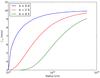 |
Fig. 2 Gas radial expansion velocity profiles for the v∞ = 10 km s-1 and b values of 0.4, 8.5 and 2.5. The model with b = 2.5 leads to the best fits to the line shape of spectra at all radial offset positions from the centre of the star. |
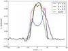 |
Fig. 3 Comparison of the H13CN(4–3) intensity profile at the centre of the star from ALMA observations and three models with b = 0.4, 2.5 and 8.5. The model with b = 2.5 reasonably fits the line spectra, while models with b = 8.5 and 0.4 are not consistent with the observations at the centre of the star. |
5.2. Radial distributions of HCN isotopologues
The molecular photodissociation by UV-radiation is the dominant process controlling HCN survival throughout the CSE. Consequently, it is the most important factor in determining the size of the HCN molecular envelope in the CSE. Since both HCN isotopologues are equally affected by UV radiation, the same molecular distribution is expected for both H12CN and H13CN isotopologues.
To estimate Re, we use the spatially resolved ALMA observations of H13CN(4−3) which strongly constrains the e-folding radius. We ran 102 models with the fixed parameters detailed in Table 2 and simultaneously varying f0 and Re over the ranges 6 × 10⁻⁷<f0< 3 × 10⁻⁶ and 1 × 10¹⁵<Re< 6 × 1015 cm (6 values for f0 and 17 values for Re). To select the model with the best Re, a reduced χ2 statistic is used. The reduced chi-square is defined as  , where 2 is the number of free parameters in our modelling. In
  calculation, we only use the average intensities at the radial offset positions (9 positions) from four directions from the centre of the star which are shown in Fig. 4. The model with the minimum has the e-folding radius Re = (2.0 ± 0.25) × 1015 cm. The cited error is for 1σ uncertainty derived from the distribution.
5.3. The H13CN abundance
To estimate the H13CN initial value f0, we use the total intensities of all three observed lines H13CN(2−1, 3−2, 4−3) in χ2 calculation. The uncertainty of the observed lines in χ2 calculation, σ, is assumed to be 20% for H13CN(2−1) APEX data, 10% for H13CN(4−3) ALMA data and 100% for H13CN(3−2) undetected line. The H13CN(3−2) undetected line was only used to put a limit on the adjustable parameters. Since various rotational transitions come from different regions of the envelope, changing the parameters in the model has a different effect on these transitions. The χ2 map is shown in Fig. 5, accompanied with the map derived using H13CN(4−3) observations to constrain the Re. The best-fitting model is chosen among the six models with Re = 2.0 × 1015 cm and 6 × 10⁻⁷<f0< 3 × 10⁻⁶, which are shown with a red line in the map. The best model with the minimum χ2 has the fractional abundance f0 = (1.9 ± 0.5) × 10-6. The H13CN spectra accompanied with the best-fitting model are presented in Fig. 6. We also compare the average intensities at the radial offset positions from ALMA observations and the best-fitting model results in Fig. 7.
Our excitation analysis shows differences between the kinetic and the excitation temperatures, meaning that all observed lines are formed under non-LTE conditions. The maximum tangential optical depth varies from ~0.09 up to 0.7 for the J = 2−1 to J = 4−3 lines, indicating that all lines are optically thin.
5.4. The H12CN abundance
To estimate the H12CN fractional abundance f0, we ran 11 models with Re = 2.0 × 1015 cm and f0 varying in the range of 1 × 10⁻⁵<f0< 6.5 × 10⁻⁵. Figure 8 shows the H12CN spectra overlaid with the best-fitting model with the minimum  . This model has a fractional abundance of f0 = (5.0 ± 2) × 10-5. In the χ2 calculation, we consider the integrated intensity of the H12CN(2−1, 3−2, 4−3) lines. Since there is evidence of maser emission in the H12CN(J = 1−0) line (e.g. Olofsson et al. 1993, 1998; Lindqvist et al. 2000; Dinh-V-Trung & Rieu 2000; Shinnaga et al. 2009; Schöier et al. 2013), we do not include in the χ2 statistic.
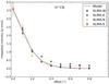 |
Fig. 4 Comparison of the integrated ALMA intensities of H13CN(4−3) at radial offset points in the CSE of R Scl towards the west, east, north and south from the centre of the star with the best-fitting model which constrains the HCN molecular distributions at Re = 2 × 1015 cm. Error-bars on the observational points show 10% uncertainty on the flux calibration. |
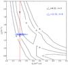 |
Fig. 5 Two |
The difference between the kinetic and the excitation temperatures for H12CN indicates that all observed lines are formed under non-LTE conditions. The maximum tangential optical depth varies from ~8 up to 30 for J = 1−0 to J = 4−3 lines, indicating that all lines are optically thick.
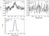 |
Fig. 6 Line emission of H13CN towards R Scl (black) overlaid with the best-fitting model (blue) which has values of f0 = 1.9 × 10⁻⁶ and Re = 2.0 × 1015 cm. Molecular transitions and the telescope used to get data are written in each panel. The H13CN(4−3) ALMA spectrum is extracted with 2′′ beam size. |
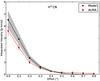 |
Fig. 7 Comparison between the average of integrated intensities of the H13CN(4−3) at radial offset positions with best-fitting model which has values of f0 = 1.9 × 10⁻⁶ and Re = 2.0 × 1015 cm. The grey region shows 1σ confidence level for Re. |
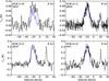 |
Fig. 8 Line emission of H12CN towards R Scl (black) overlaid with the best-fitting model (blue). Molecular transitions and the telescope used to get data are written in each panel. Second peaks in J= 2−1, 3−2, 4−3 transitions are due to maser emission in the (011c0) vibrational state. |
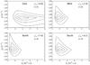 |
Fig. 9 Comparison between four |
6. Discussion
6.1. Comparison of the best-fitting criteria based on single-dish and interferometric observations
Comparison between two χ2 maps in Fig. 5 shows that the best-fitting criteria based on the high-resolution interferometric and low-resolution single-dish observations are different. The single-dish observations require a larger e-folding radius with less fractional abundance, while interferometric observations require a more compact envelope with higher abundance. This illustrates the importance of spatially resolved images of even a subset of the transitions used in molecular modelling. For comparison, a model selected only on the single-dish spectra is presented in the Appendix.
The H12CN modelling for R Scl by W04 also implements the different best-fitting criteria based on the single-dish and interferometric observations. They require a more compact envelope with less abundance to fit the spatially-resolved H12CN(1−0) ATCA observations, while they can not fit the single-dish spectra using the same condition (see Figs. 7 and 8 in W04).
A possible explanation for this discrepancy might be the spherically symmetric molecular distribution considered in our models, especially considering R Scl is known to have a binary companion whose influence gives rise to the spiral pattern observed in CO (Maercker et al. 2012). Constraining this asymmetry in the inner wind is, with the currently available observations, not yet possible. However, while the asymmetry could affect the derived abundances, it does not affect our determination of the isotopologue ratio, which is the main aim of this work.
6.2. Asymmetry in the CSE
Our modelling is based on assuming a spherically symmetric envelope around R Scl. This is a first order approximation, and the east-west asymmetry in the CSE as seen in Fig. 1 possibly due to the binary companion is not taken into account. Indeed, we are not able to precisely constrain the additional free parameters required to fully describe the physical condition such as the molecular distribution profiles from the available data. To find out the effect of this asymmetry in determining the adjustable parameters, we calculate the statistic in four directions from the central star. As seen in Fig. 9, in west, north and south lead to approximately the same range of adjustable parameters, while the contour map from the east shows a larger Re, which is expected to be due to the elongation of the molecular gas towards the east as seen also in Fig. 1.
The east-west elongation of the molecular distribution could also be an explanation of the underestimate of the lower-J HCN emission. Assuming that the lower-J transitions are predominantly excited in the more extended aspherical region, a spherical symmetric model will either overestimate the lower-J transitions when adopting the large Re found in the east-west direction, or underestimate them when adopting a smaller average Re.
6.3. Comparison with previous studies
We compared our results with those of previous studies. The H12CN circumstellar abundance value of (5.0 ± 2) × 10-5 reported here for R Scl is higher than previously reported values of 8.1 × 10⁻⁶ and 1.2 × 10⁻⁵ by Olofsson et al. (1993) and W04, respectively. It should be noted that Olofsson et al. (1993) derived their abundance through a different method (see Eq. (3) in Olofsson et al. 1993). However, our result is consistent with the median value of the H12CN fractional abundances f0 = 3.0 ×10⁻⁵ for a sample of 25 carbon stars studied by Schöier et al. (2013) and the average value of f0 = 4.6 ×10⁻⁵ for a sample of five carbon stars studied by Lindqvist et al. (2000). The derived H12CN abundance here is also in good agreement with results of LTE stellar atmosphere models f = (1−5) × 10-5 reported for carbon-type stars by Willacy & Cherchneff (1998) and Cherchneff (2006).
The e-folding radius of Re = (2.0 ± 0.25) ×1015 cm derived here is smaller than the values reported by W04 and Olofsson et al. (1993) (r = 1.5 × 1016 cm and r = 3.6 × 1015 cm, respectively). However, the result reported in Olofsson et al. (1993) is not based on solving the radiative transfer equation (see Eq. (6) in Olofsson et al. 1993). The excitation analysis of W04 considered a fixed fHCN throughout the envelope out to the outer radius r = 1.5 × 1016 cm to fit the multi-transition spectra. However this radius is not consistent with the J = 1−0 ATCA intensity map, which requires a smaller envelope of r = 5.5 × 1015 cm and a higher photospheric abundance.
We speculate that the difference between the two envelope sizes derived based on the interferometric observations of H12CN(1−0) by W04 (~360 AU) and H13CN(4−3) here (~130 AU) could be due to the influence of the binary companion at ~60 AU. As seen in CO in the outer envelope, the binary interaction causes a spiral density pattern that will alter the physical conditions in the outflow. The relative magnitude of the density pattern grows rapidly beyond the binary companion (e.g. Kim & Taam 2012) and the east-west HCN extension could be the observational indication of the start of the density pattern. The wave might have a stronger effect on the excitation of H12CN(1−0) than that of H13CN(4−3).
6.4. Comparison of the isotopologue ratios
We have derived a ratio of circumstellar H12CN/H13CN = 26.3 ± 11.9 for R Scl which is consistent with the photospheric atomic carbon ratio of 12C/13C ~ 19 ± 6 reported by Lambert et al. (1986). The derived isotopologue ratio is not affected by the limitation in the modelling (e.g. considering the effects of the binary companion on the physical condition), since the abundances are equally affected by these limitations.
The CN molecule is also photodissociated in the continuum (el-Qadi & Stancil 2013). Hence, the 12CN/13CN isotopologue ratio is expected to follow the 12C/13C isotopic ratio. An intensity ratio of 12CN(1−0)/13CN(1−0) ~ 24 for R Scl reported by Olofsson et al. (1996) is consistent with the photospheric 12C/13C and the H12CN/H13CN ratio reported here.
At the same time, the authors of V13 find an average value of 12CO/13CO ~ 19 in the detached shell, consistent with the atomic carbon photospheric estimates, whereas they derive a lower limit of 12CO/13CO > 60 for the present-day mass loss.
Since H12CN/H13CN and 12CN/13CN ratios are consistent with the 12C/13C ratio, the most probable scenario of explaining the unexpectedly high 12CO/13CO ratio in the inner CSE of R Scl is CO isotopologue selective-shielding. The extra photodissociation of less abundant 13CO is most likely by the internal UV radiation as proposed by V13.
In addition, Olofsson et al. (1996) have reported an intensity ratio of 12CN(1−0)/H12CN(1−0) ~4.3 which is higher by a factor of two from the average value 2.0 ± 0.7 reported for C-type stars. Assuming that HCN photodissociation is solely responsible for producing CN in the circumstellar environment, the ratio reported by Olofsson et al. (1996) also supports the extra UV radiation in the CSE of R Scl.
Consequently, taking isotopologue self-shielding of molecules which are dissociated in discrete bands in the UV, e.g. 12CO/13CO, into account is very important in the determination of the isotopologue ratios. Moreover, the isotopologue ratios of these molecules are not always a reliable tracer of the atomic carbon isotope ratio 12C/13C in UV irradiated regions. The discrepancy between the two ratios can be considerable in optically thick regions where the isotopologue self-shielding has more impact.
7. Conclusion
We have performed a detailed non-LTE excitation analysis of H12CN and H13CN in the CSE of R Scl. The derived H12CN/H13CN = 26.3 ± 11.9 is consistent with the photospheric ratio of 12C/13C ~ 19 ± 6 reported by Lambert et al. (1986).
It is clearly shown that constraining the molecular distribution size, the fractional abundance and the radial expansion velocity profile in the CSE requires high-resolution spatially-resolved observations.
Our results show that the circumstellar H12CN/H13CN ratio is a more reliable tracer of the photospheric 12C/13C ratio than the circumstellar 12CO/13CO ratio in the UV irradiated region. These results also support the isotopologue selective-shielding of CO as the reason for the lacking of 13CO in the inner CSE of R Scl as previously claimed by V13. The extra photodissociation of 13CO is most likely due to the internal radiation either from the binary companion or chromospheric activity. This indicates the important role of internal UV radiation as well as the ISRF on the chemical composition of the CSEs. Thus, should be considered in the chemical-physical modelling of the CSEs around evolved stars.
In a more general context, the most abundant molecules in astrophysical regions that control the chemistry, for example H2, CO, N2, C2H2, have sharp discrete absorption bands in UV (Lee 1984), which leads to isotopic fractionation in the UV irradiated regions. Thus, considering the isotopologue selective-shielding is very important in astrochemical models of AGB envelopes and other irradiated environments.
We suggest that the comparison between the photospheric 12C/13C ratio and the circumstellar 12CO/13CO and H12CN/H13CN ratios can indirectly trace the internal embedded UV sources, which are difficult to observe directly, in the CSEs of evolved stars.
This comparison cannot distinguish between the contributions from different potential UV sources such as ISRF, the chromospheric activity and active binary companions. This requires spatially-resolved observations of the photodissociated products such as atomic carbon.
XS is a package developed by P. Bergman to reduce and analyse single-dish spectra. It is publicly available from ftp://yggdrasil.oso.chalmers.se
Acknowledgments
This paper makes use of ALMA data from project No. ADS/JAO.ALMA#2012.1.00097.S. ALMA is a partnership of ESO (representing its member states), the NSF (USA) and NINS (Japan), together with the NRC (Canada), NSC and ASIAA (Taiwan) and KASI (Republic of Korea), in cooperation with the Republic of Chile. The Joint ALMA Observatory is operated by ESO, AUI/NRAO and NAOJ. This work is supported by ERC consolidator grant 614264. M.M. has received funding from the People Programme (Marie Curie Actions) of the EU’s FP7 (FP7/2007–2013) under REA grant agreement No. 623898.11.
References
- Agúndez, M., Cernicharo, J., & Guélin, M. 2010, ApJ, 724, L133 [NASA ADS] [CrossRef] [Google Scholar]
- Bieging, J. H. 2001, ApJ, 549, L125 [NASA ADS] [CrossRef] [Google Scholar]
- Bieging, J. H., Chapman, B., & Welch, W. J. 1984, ApJ, 285, 656 [NASA ADS] [CrossRef] [Google Scholar]
- Bujarrabal, V., Fuente, A., & Omont, A. 1994, A&A, 285, 247 [NASA ADS] [Google Scholar]
- Castro-Carrizo, A., Quintana-Lacaci, G., Neri, R., et al. 2010, A&A, 523, A59 [NASA ADS] [CrossRef] [EDP Sciences] [Google Scholar]
- Cherchneff, I. 2006, A&A, 456, 1001 [NASA ADS] [CrossRef] [EDP Sciences] [Google Scholar]
- Cherchneff, I. 2012, A&A, 545, A12 [NASA ADS] [CrossRef] [EDP Sciences] [Google Scholar]
- Danilovich, T., Bergman, P., Justtanont, K., et al. 2014, A&A, 569, A76 [NASA ADS] [CrossRef] [EDP Sciences] [Google Scholar]
- De Beck, E., Decin, L., de Koter, A., et al. 2010, A&A, 523, A18 [NASA ADS] [CrossRef] [EDP Sciences] [Google Scholar]
- De Beck, E., Lombaert, R., Agúndez, M., et al. 2012, A&A, 539, A108 [NASA ADS] [CrossRef] [EDP Sciences] [Google Scholar]
- Decin, L., De Beck, E., Brünken, S., et al. 2010, A&A, 516, A69 [NASA ADS] [CrossRef] [EDP Sciences] [Google Scholar]
- Dinh-V-Trung, & Rieu, N.-Q. 2000, A&A, 361, 601 [NASA ADS] [Google Scholar]
- Eaton, J. A., & Johnson, H. R. 1988, ApJ, 325, 355 [NASA ADS] [CrossRef] [Google Scholar]
- el-Qadi, W. H., & Stancil, P. C. 2013, ApJ, 779, 97 [NASA ADS] [CrossRef] [Google Scholar]
- González Delgado, D., Olofsson, H., Schwarz, H. E., Eriksson, K., & Gustafsson, B. 2001, A&A, 372, 885 [NASA ADS] [CrossRef] [EDP Sciences] [Google Scholar]
- González Delgado, D., Olofsson, H., Schwarz, H. E., et al. 2003, A&A, 399, 1021 [NASA ADS] [CrossRef] [EDP Sciences] [Google Scholar]
- Greaves, J. S., & Holland, W. S. 1997, A&A, 327, 342 [NASA ADS] [Google Scholar]
- Groenewegen, M. A. T., Baas, F., de Jong, T., & Loup, C. 1996, A&A, 306, 241 [NASA ADS] [Google Scholar]
- Habing, H. J. 1996, A&ARv, 7, 97 [NASA ADS] [CrossRef] [Google Scholar]
- Habing, H. J., & Olofsson, H. 2003, Asymptotic giant branch stars (New York, Berlin: Springer) [Google Scholar]
- Johnson, H. R., Baumert, J. H., Querci, F., & Querci, M. 1986, ApJ, 311, 960 [NASA ADS] [CrossRef] [Google Scholar]
- Kim, H., & Taam, R. E. 2012, ApJ, 759, L22 [NASA ADS] [CrossRef] [Google Scholar]
- Knapp, G. R., Pourbaix, D., Platais, I., & Jorissen, A. 2003, A&A, 403, 993 [NASA ADS] [CrossRef] [EDP Sciences] [Google Scholar]
- Lambert, D. L., Gustafsson, B., Eriksson, K., & Hinkle, K. H. 1986, ApJS, 62, 373 [NASA ADS] [CrossRef] [Google Scholar]
- Lee, L. C. 1984, ApJ, 282, 172 [NASA ADS] [CrossRef] [Google Scholar]
- Lindqvist, M., Schöier, F. L., Lucas, R., & Olofsson, H. 2000, A&A, 361, 1036 [NASA ADS] [Google Scholar]
- Maercker, M., Schöier, F. L., Olofsson, H., Bergman, P., & Ramstedt, S. 2008, A&A, 479, 779 [NASA ADS] [CrossRef] [EDP Sciences] [Google Scholar]
- Maercker, M., Schöier, F. L., Olofsson, H., et al. 2009, A&A, 494, 243 [NASA ADS] [CrossRef] [EDP Sciences] [Google Scholar]
- Maercker, M., Mohamed, S., Vlemmings, W. H. T., et al. 2012, Nature, 490, 232 [NASA ADS] [CrossRef] [PubMed] [Google Scholar]
- Maercker, M., Ramstedt, S., Leal-Ferreira, M. L., Olofsson, G., & Floren, H. G. 2014, A&A, 570, A101 [NASA ADS] [CrossRef] [EDP Sciences] [Google Scholar]
- Maercker, M., Danilovich, T., Olofsson, H., et al. 2016a, A&A, 591, A44 [Google Scholar]
- Maercker, M., Vlemmings, W. H. T., Brunner, M., et al. 2016b, A&A, 586, A5 [NASA ADS] [CrossRef] [EDP Sciences] [Google Scholar]
- Milam, S. N., Woolf, N. J., & Ziurys, L. M. 2009, ApJ, 690, 837 [NASA ADS] [CrossRef] [Google Scholar]
- Neri, R., Kahane, C., Lucas, R., Bujarrabal, V., & Loup, C. 1998, A&AS, 130, 1 [NASA ADS] [CrossRef] [EDP Sciences] [Google Scholar]
- Olofsson, H., Eriksson, K., Gustafsson, B., & Carlstrom, U. 1993, ApJS, 87, 267 [NASA ADS] [CrossRef] [Google Scholar]
- Olofsson, H., Bergman, P., Eriksson, K., & Gustafsson, B. 1996, A&A, 311, 587 [NASA ADS] [Google Scholar]
- Olofsson, H., Lindqvist, M., Nyman, L.-A., & Winnberg, A. 1998, A&A, 329, 1059 [NASA ADS] [Google Scholar]
- Olofsson, H., Maercker, M., Eriksson, K., Gustafsson, B., & Schöier, F. 2010, A&A, 515, A27 [NASA ADS] [CrossRef] [EDP Sciences] [Google Scholar]
- Omont, A., Loup, C., Forveille, T., et al. 1993, A&A, 267, 515 [NASA ADS] [Google Scholar]
- Ortiz, R., & Guerrero, M. A. 2016, MNRAS, 461, 3036 [Google Scholar]
- Quintana-Lacaci, G., Agúndez, M., Cernicharo, J., et al. 2016, A&A, 592, A51 [NASA ADS] [CrossRef] [EDP Sciences] [Google Scholar]
- Ramstedt, S., Schöier, F. L., Olofsson, H., & Lundgren, A. A. 2008, A&A, 487, 645 [NASA ADS] [CrossRef] [EDP Sciences] [Google Scholar]
- Rybicki, G. B., & Hummer, D. G. 1991, A&A, 245, 171 [NASA ADS] [Google Scholar]
- Sahai, R., Findeisen, K., Gil de Paz, A., & Sánchez Contreras, C. 2008, ApJ, 689, 1274 [NASA ADS] [CrossRef] [Google Scholar]
- Savage, B. D., & Sembach, K. R. 1996, ARA&A, 34, 279 [NASA ADS] [CrossRef] [Google Scholar]
- Schöier, F. L., & Olofsson, H. 2000, A&A, 359, 586 [NASA ADS] [Google Scholar]
- Schöier, F. L., & Olofsson, H. 2001, A&A, 368, 969 [NASA ADS] [CrossRef] [EDP Sciences] [Google Scholar]
- Schöier, F. L., Maercker, M., Justtanont, K., et al. 2011, A&A, 530, A83 [NASA ADS] [CrossRef] [EDP Sciences] [Google Scholar]
- Schöier, F. L., Ramstedt, S., Olofsson, H., et al. 2013, A&A, 550, A78 [NASA ADS] [CrossRef] [EDP Sciences] [Google Scholar]
- Shinnaga, H., Young, K. H., Tilanus, R. P. J., et al. 2009, ApJ, 698, 1924 [NASA ADS] [CrossRef] [Google Scholar]
- Visser, R., van Dishoeck, E. F., & Black, J. H. 2009, A&A, 503, 323 [NASA ADS] [CrossRef] [EDP Sciences] [Google Scholar]
- Vlemmings, W. H. T., Maercker, M., Lindqvist, M., et al. 2013, A&A, 556, L1 [NASA ADS] [CrossRef] [EDP Sciences] [Google Scholar]
- Watson, W. D., Anicich, V. G., & Huntress, Jr., W. T. 1976, ApJ, 205, L165 [NASA ADS] [CrossRef] [Google Scholar]
- Whitelock, P. A., Feast, M. W., & van Leeuwen, F. 2008, MNRAS, 386, 313 [NASA ADS] [CrossRef] [Google Scholar]
- Willacy, K., & Cherchneff, I. 1998, A&A, 330, 676 [NASA ADS] [Google Scholar]
- Wong, T., Schöier, F. L., Lindqvist, M., & Olofsson, H. 2004, A&A, 413, 241 [NASA ADS] [CrossRef] [EDP Sciences] [Google Scholar]
Appendix A
An example model which fits the total intensities of H13CN(2–1, 4–3) spectra very well, but is not consistent with the integrated intensities at radial offset positions from ALMA observations, Figs. A.1 and A.2. This model has a radial expansion velocity profile with values b = 0.5 and V∞ = 8.5. As it was mentioned in Sect. 5.1, the models with b < 2.5 give a double peak shape intensity profiles in the inner part ( ). Figure A.3 shows the intensity profile at the central point of the star from the model and ALMA observations. This model has a larger abundance of f0 = 8.0 × 10⁻⁷ and a smaller radius of Re = 5.0 × 1015 cm compared to our best model which was discussed in Sect. 5. Thus, the best-fitting criteria based on the single-dish observations requires a smaller envelope and larger abundance. This model shows the importance of using spatially resolved interferometric data in constraining the adjustable parameters in the modelling of the CSE.
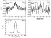 |
Fig. A.1 Line emission of H13CN towards R Scl (black) overlaid with the model results (blue). Molecular transitions and the telescope used to get data are written in each panel. |
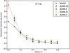 |
Fig. A.2 Comparison of the ALMA integrated intensities of H13CN(4−3) at radial offset points in the CSE of R Scl towards the west, east, north and south from the centre of the star with the model results. Error-bars on the observational points show 10% uncertainty on the flux calibration. |
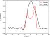 |
Fig. A.3 Comparison of the H13CN(4–3) line emission towards R Scl at the centre of the star from ALMA observations and a model with fast accelerating wind (b = 0.5). |
All Tables
Stellar parameters used in the radiative transfer modelling of the H12CN and H13CN isotopologues around R Scl.
All Figures
|
Fig. 1 Zero-moment H13CN(4–3) map of R Scl observed with ALMA. The ALMA beam size is shown in the bottom left corner. |
| In the text | |
|
Fig. 2 Gas radial expansion velocity profiles for the v∞ = 10 km s-1 and b values of 0.4, 8.5 and 2.5. The model with b = 2.5 leads to the best fits to the line shape of spectra at all radial offset positions from the centre of the star. |
| In the text | |
|
Fig. 3 Comparison of the H13CN(4–3) intensity profile at the centre of the star from ALMA observations and three models with b = 0.4, 2.5 and 8.5. The model with b = 2.5 reasonably fits the line spectra, while models with b = 8.5 and 0.4 are not consistent with the observations at the centre of the star. |
| In the text | |
|
Fig. 4 Comparison of the integrated ALMA intensities of H13CN(4−3) at radial offset points in the CSE of R Scl towards the west, east, north and south from the centre of the star with the best-fitting model which constrains the HCN molecular distributions at Re = 2 × 1015 cm. Error-bars on the observational points show 10% uncertainty on the flux calibration. |
| In the text | |
|
Fig. 5 Two |
| In the text | |
|
Fig. 6 Line emission of H13CN towards R Scl (black) overlaid with the best-fitting model (blue) which has values of f0 = 1.9 × 10⁻⁶ and Re = 2.0 × 1015 cm. Molecular transitions and the telescope used to get data are written in each panel. The H13CN(4−3) ALMA spectrum is extracted with 2′′ beam size. |
| In the text | |
|
Fig. 7 Comparison between the average of integrated intensities of the H13CN(4−3) at radial offset positions with best-fitting model which has values of f0 = 1.9 × 10⁻⁶ and Re = 2.0 × 1015 cm. The grey region shows 1σ confidence level for Re. |
| In the text | |
|
Fig. 8 Line emission of H12CN towards R Scl (black) overlaid with the best-fitting model (blue). Molecular transitions and the telescope used to get data are written in each panel. Second peaks in J= 2−1, 3−2, 4−3 transitions are due to maser emission in the (011c0) vibrational state. |
| In the text | |
|
Fig. 9 Comparison between four |
| In the text | |
|
Fig. A.1 Line emission of H13CN towards R Scl (black) overlaid with the model results (blue). Molecular transitions and the telescope used to get data are written in each panel. |
| In the text | |
|
Fig. A.2 Comparison of the ALMA integrated intensities of H13CN(4−3) at radial offset points in the CSE of R Scl towards the west, east, north and south from the centre of the star with the model results. Error-bars on the observational points show 10% uncertainty on the flux calibration. |
| In the text | |
|
Fig. A.3 Comparison of the H13CN(4–3) line emission towards R Scl at the centre of the star from ALMA observations and a model with fast accelerating wind (b = 0.5). |
| In the text | |
Current usage metrics show cumulative count of Article Views (full-text article views including HTML views, PDF and ePub downloads, according to the available data) and Abstracts Views on Vision4Press platform.
Data correspond to usage on the plateform after 2015. The current usage metrics is available 48-96 hours after online publication and is updated daily on week days.
Initial download of the metrics may take a while.