| Issue |
A&A
Volume 598, February 2017
|
|
|---|---|---|
| Article Number | A25 | |
| Number of page(s) | 22 | |
| Section | Cosmology (including clusters of galaxies) | |
| DOI | https://doi.org/10.1051/0004-6361/201629626 | |
| Published online | 26 January 2017 | |
QuickPol: Fast calculation of effective beam matrices for CMB polarization
1 Sorbonne Universités, UPMC Univ. Paris 6 & CNRS (UMR 7095): Institut d’Astrophysique de Paris, 98bis boulevard Arago, 75014 Paris, France
e-mail: This email address is being protected from spambots. You need JavaScript enabled to view it.
2 Institut de Planétologie et d’Astrophysique de Grenoble, Université Grenoble Alpes, CNRS (UMR 5274), 38000 Grenoble, France
3 Institut d’Astrophysique Spatiale, CNRS (UMR 8617) Université Paris-Sud 11, Bâtiment 121, 91405 Orsay, France
Received: 31 August 2016
Accepted: 2 October 2016
Abstract
Current and planned observations of the cosmic microwave background (CMB) polarization anisotropies, with their ever increasing number of detectors, have reached a potential accuracy that requires a very demanding control of systematic effects. While some of these systematics can be reduced in the design of the instruments, others will have to be modeled and hopefully accounted for or corrected a posteriori. We propose QuickPol, a quick and accurate calculation of the full effective beam transfer function and of temperature to polarization leakage at the power spectra level, as induced by beam imperfections and mismatches between detector optical and electronic responses. All the observation details such as exact scanning strategy, imperfect polarization measurements, and flagged samples are accounted for. Our results are validated on Planck high frequency instrument (HFI) simulations. We show how the pipeline can be used to propagate instrumental uncertainties up to the final science products, and could be applied to experiments with rotating half-wave plates.
Key words: cosmic background radiation / cosmology: observations / polarization / methods: analytical
© ESO, 2017
1. Introduction
We are now entering an era of precise measurements of the cosmic microwave background (CMB) polarization, with potentially enough sensitivity to detect or even characterize the primordial tensorial B modes, the smoking gun of inflation (e.g., Zaldarriaga & Seljak 1997, and references therein). This raises expectations about the control and the correction of contaminations by astrophysical foregrounds, observational features, and instrumental imperfections. As it has in the past, progress will come from the synergy between instrumentation and data analysis. Improvements in instrumentation call for improved precision in final results, which are made possible by improved algorithms and the ability to deal with more and more massive data sets. In turn, expertise gained in data processing allows for better simulations that lead to new instrument designs and better suited observations. An example of such joint developments is the study of the impact of optics- and electronics-related imperfections on the measured CMB temperature and polarization angular power spectra and their statistical isotropy. Systematic effects such as beam non-circularity, response mismatch in dual polarization measurements and scanning strategy imperfections, as well as how they can be mitigated, have been extensively studied in the preparation of forthcoming instruments (including, but not limited to Souradeep & Ratra 2001; Fosalba et al. 2002; Hu et al. 2003; Mitra et al. 2004, 2009; O’Dea et al. 2007; Rosset et al. 2007; Shimon et al. 2008; Miller et al. 2009a,b; Hanson et al. 2010; Leahy et al. 2010; Rosset et al. 2010; Ramamonjisoa et al. 2013; Rathaus & Kovetz 2014; Wallis et al. 2014; Pant et al. 2016), and during the analysis of data collected by WMAP1 (Smith et al. 2007; Hinshaw et al. 2007; Page et al. 2007) or Planck2 (Planck Collaboration VII 2014; Planck Collaboration XVII 2014; Planck Collaboration XI 2016) satellite missions.
At the same time, several deconvolution algorithms and codes have been proposed to clean up the CMB maps from such beam-related effects prior to the computation of the power spectra, like PreBeam (Armitage-Caplan & Wandelt 2009), ArtDeco (Keihänen & Reinecke 2012), and in Bennett et al. (2013) and Wallis et al. (2015), or during their production (Keihänen et al. 2016).
Finally, in a related effort, the FEBeCoP pipeline, described in Mitra et al. (2011) and used in Planck data analysis (Planck Collaboration IV 2014; Planck Collaboration VII 2014), can be seen as a convolution facility, by providing, at arbitrary locations on the sky, the effective beam maps and point spread functions of a detector set, which, in turn, can be used for a Monte-Carlo based description of the effective beam window functions for a given sky model.
In this paper, we introduce the QuickPol pipeline, an extension to polarization of the Quickbeam algorithm used in Planck Collaboration VII (2014). It allows a quick and accurate computation of the leakage and cross-talk between the various temperature and polarization power spectra (TT, EE, BB, TE, etc.) taking into account the exact scanning, sample flags, relative weights, and scanning beams of the considered set(s) of detectors. The end results are effective beam matrices describing, for each multipole ℓ, the mixing of the various spectra, independently of the actual value of the spectra. As we shall see, the impact of changing any time-independent feature of the instrument, such as its beam maps, relative gain calibrations, detector orientations, and polarization efficiencies can be propagated within seconds to the final beam matrices products, allowing extremely fast Monte-Carlo exploration of the experimental features. QuickPol is thus a powerful tool for both real data analysis and forthcoming experiments, simulations and design.
The paper is organized as follows. The mathematical formalism is exposed in Sect. 2 and analytical results are given in Sect. 3. The numerical implementation is detailed in Sect. 4 and compared to the results of Planck simulations in Sect. 5. Section 6 shows the propagation of instrumental uncertainties. We discuss briefly the case of rotating half-wave plates in Sect. 7 and conclude in Sect. 8.
2. Formalism
2.1. Data stream of a polarized detector
As usual in the study of polarization measurement, we will use Jones’ formalism to study the evolution of the electric component of an electro-magnetic radiation in the optical system. Let us consider a quasi monochromatic3 radiation propagating along the z axis, and hitting the optical system at a position  . The incoming electric field
  will be turned into e′(r) = J(r).e(r), where J(r) is the 2 × 2 complex Jones matrix of the system.
A rotation of the optical system by α around the z axis can be seen as a rotation of both the orientation and location of the incoming radiation by −α in the detector reference frame, and the same input radiation is now received as  (1)with
  and the † sign representing the adjoint operation, which for a real rotation matrix, simply amounts to the matrix transpose. The measured signal is
  (4)with
  (5)We now introduce the Stokes parameters of the input signal (dropping the dependence on r)
 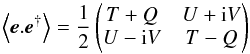 (6)and of the (un-rotated) instrument response
 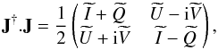 (7)to obtain
![Mathematical equation: \begin{eqnarray} {\rm d}(\alpha) = \frac{1}{2} \int {\rm d}\vecr \left[ \bI (\alpha, \vecr)T(\vecr) +\bQ (\alpha, \vecr)Q(\vecr) +\bU (\alpha, \vecr)U(\vecr) -\bV (\alpha, \vecr)V(\vecr) \right]. \label{eq:datastream_beam} \end{eqnarray}](/articles/aa/full_html/2017/02/aa29626-16/aa29626-16-eq23.png) (8)With the rotated instrument response:
(8)With the rotated instrument response: 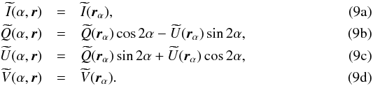 Following Rosset et al. (2010), we can specify the instrument as being a beam forming optics, followed by an imperfect polarimeter in the direction x, with 0 ≤ η ≤ 1, and having an overall optical efficiency 0 ≤ τ ≤ 1:
 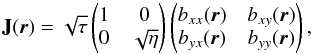 (10)with
 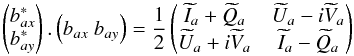 (11)for a = x,y. The Stokes parameters of the instrument are then
  for
for  .
.
If the beam is assumed to be perfectly co-polarized, that is, it does not alter at all the polarization of the incoming radiation, with bxy = byx = 0 and bxx = byy, then  ,
,  , and
, and  ,
,  ,
,  , Eqs. ((8), (9)) become
 ![Mathematical equation: \begin{equation} {\rm d}(\alpha) = \frac{1+\eta}{2} \tau \int {\rm d}\vecr \bI_x(\vecr_\alpha) \left[ T(\vecr) + \cpe\left(Q(\vecr)\cos2\alpha + U(\vecr)\sin2\alpha\right) \right], \label{eq:datastream_copolar} \end{equation}](/articles/aa/full_html/2017/02/aa29626-16/aa29626-16-eq40.png) (12)where
(12)where  (13)is the polar efficiency, such that 0 ≤ ρ ≤ 1 with ρ = 1 for a perfect polarimeter and ρ = 0 for a detector only sensitive to intensity. In the case of Planck high frequency instrument (HFI), Rosset et al. (2010) showed the measured polarization efficiencies to differ by Δρ′ = 1% to 16% from their ideal values, with an absolute statistical uncertainty generally below 1%. The particular case of co-polarized beams is important because in most experimental setups, such as Planck, the beam response calibration is done on astronomical or artificial far field sources. Well known, compact, and polarized sources are generally not available to measure
  and
and  and only the intensity beam response
  is measured. In the absence of reliable physical optics modeling of the beam response, one therefore has to assume and to be perfectly co-polarized.
So far, we have only considered the optical beam response. We should also take into account the scanning beam, which is the convolution of the optical beam with the finite time response of the instrument (or its imperfect correction) as it moves around the sky, as described in Planck Collaboration VII (2014) and Planck Collaboration VII (2016). These time related effects can be a major source of elongation of the scanning beams, and can increase the beam mismatch among sibling detectors. If one assumes the motion of the detectors on the sky to be nearly uniform, as was the case for Planck, then optical beams can readily be replaced by scanning beams in the QuickPol formalism.
2.2. Spherical harmonics analysis
We now define the tools that are required to extend the above results to the full celestial sphere. The temperature T is a scalar quantity, while the linear polarization Q ± iU is of spin ± 2, and the circular polarization V is generally assumed to vanish. They can be written as linear combinations of spherical harmonics (SH): 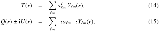 although one usually prefers the scalar and fixed parity E and B components
  (16)such that
  for X = T,E,B. In other terms
 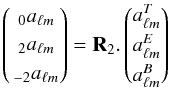 (17)with
  (18)The sign convention used in Eq. (16) is consistent with Zaldarriaga & Seljak (1997) and the HEALPix4 library (Górski et al. 2005).
The response of a beam centered on the North pole can also be decomposed in SH coefficients  while the coefficients of a rotated beam can be computed by noting that under a rotation of angle α around the direction r, the SH of spin s transform as
  (21)The elements of Wigner rotation matrices D are related to the SH via (Challinor et al. 2000)
  (22)with
  .
.
If the beam is assumed to be co-polarized and coupled with a perfect polarimeter rotated by an angle γ, such that  in Cartesian coordinates (or
  in (θ,φ) polar coordinates), simple relations between bℓm and
  can be established. For a Gaussian circular beam of full width half maximum (FWHM)
  and of throughput
  Challinor et al. (2000) found
  The factor c2 = e2σ2 in Eq. (23b) is such that c2−1 < 1.1 × 10⁻⁴ for θFWHM ≤ 1° and c2−1 < 3.1 × 10⁻⁶ for θFWHM ≤ 10′, and will be assumed to be c2 = 1 from now on. For a slightly elliptical Gaussian beam, Fosalba et al. (2002) found
  (24)while we show in Appendix G that Eq. (24) is true for arbitrarily shaped co-polarized beams. This result can also be obtained by noting that an arbitrary beam is the sum of Gaussian circular beams with different FWHM and center (Tristram et al. 2004), each of them obeying Eq. (23b).
The detector associated to a beam is an imperfect polarimeter with a polarization efficiency ρ′ and the overall polarized response of the detector, in a referential aligned with its direction of polarization (the so-called Pxx coordinates in Planck parlance), reads  (25)so that
  (26)We introduced ρ′ to distinguish it from the ρ value used in the map-making, as described below.
2.3. Map making equation
A polarized detector pointing, at time t, in the direction rt on the sky, and being sensitive to the polarization with angle αt with respect to the local meridian, measures ![Mathematical equation: \begin{eqnarray} {\rm d}(\vecr_t,\alpha_t) = \int \dd\vecr' \left[\bI(\vecr_t,\alpha_t; \vecr') T(\vecr') + \bQ(\vecr_t,\alpha_t; \vecr') Q(\vecr') + \bU(\vecr_t,\alpha_t; \vecr') U(\vecr') \right]. \label{eq:TODanybeam} \end{eqnarray}](/articles/aa/full_html/2017/02/aa29626-16/aa29626-16-eq89.png) (27)The factor 1/2 present in Eq. (8) is assumed to be absorbed in the gain calibration, performed on large scale temperature fluctuations, such as the CMB solar dipole (Planck Collaboration VIII 2014), and we assumed the circular polarization V to vanish. With the definitions introduced in Sect. 2.2, this becomes
(27)The factor 1/2 present in Eq. (8) is assumed to be absorbed in the gain calibration, performed on large scale temperature fluctuations, such as the CMB solar dipole (Planck Collaboration VIII 2014), and we assumed the circular polarization V to vanish. With the definitions introduced in Sect. 2.2, this becomes ![Mathematical equation: \begin{eqnarray} {\rm d}(\vecr_t,\alpha_t) = \sum_{\ell ms} \left[ _{0} a_{\ell m}\ _{0} b^{*}_{\ell s} + 1/2\left( _{2} a_{\ell m}\ _{2} b^{*}_{\ell s} + \ _{-2} a_{\ell m}\ _{-2} b^{*}_{\ell s} \right)\right] (-1)^s\, q_{\ell}\, {\rm e}^{{\rm i}s\alpha_t} \ _{-s}Y_{\ell m}(\vecr_t). \label{eq:TOD_from_alm} \end{eqnarray}](/articles/aa/full_html/2017/02/aa29626-16/aa29626-16-eq91.png) (28)The map-making formalism is set ignoring the beam effects, assuming a perfectly co-polarized detector and an instrumental noise n (Tristram et al. 2011, and references therein), so that, for a detector j, Eq. (12) becomes
(28)The map-making formalism is set ignoring the beam effects, assuming a perfectly co-polarized detector and an instrumental noise n (Tristram et al. 2011, and references therein), so that, for a detector j, Eq. (12) becomes  (29)where the leading prefactors are here again absorbed in the gain calibration. Let us rewrite it as
 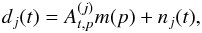 (30)with (Shimon et al. 2008)
 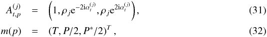 and P = Q + iU. Assuming the noise to be uncorrelated between detectors, with covariance matrix
  for detector j, the generalized least square solution of Eq. (29) for a set of detectors is
 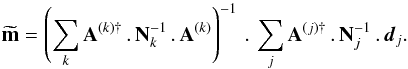 (33)Let us now replace the ideal data stream (Eq. (29)) with the one obtained for arbitrary beams (Eq. (27)) and further assume that the noise is white and stationary with variance
  , so that
  . Let us also introduce the binary flag fj,t used to reject individual time samples from the map-making process; Eq. (33) then becomes
  We have assumed here the pixels to be infinitely small, so that, starting with Eq. (28), the location of all samples in a pixel coincides with the pixel center. The effect of the pixel’s finite size and the so-called sub-pixel effects will be considered in Sect. 3.5.
2.4. Measured power spectra
To compute the cross-power spectrum of any two spin v1 and v2 maps, we first project each polarized component v of  on the appropriate spin weighted sets of spherical harmonics,
  (36)and average these terms according to
  where Eq. (C.6) was used. The detailed derivation of this relation and its associated terms is given in Appendix A. Suffice it to say here that ku terms are either 1 or 1/2,
  terms are inverse noise-weighted beam multipoles, and
  terms are effective weights describing the scanning and depending on the direction of polarization, hit redundancy (both from sky coverage and flagged samples), and noise level of detector j.
Equation (38) is therefore a generalization to non-circular beams of the pseudo-power spectra measured on a masked or weighted map (Hivon et al. 2002; Hansen & Górski 2003), and extends to polarization the Quickbeam non-circular beam formalism used in the data analysis conducted by Planck Collaboration VII (2014). It also formally agrees with Hu et al. (2003)’s results on the impact of systematic effects on the polarization power spectra, with the functions  absorbing the systematic effect parameters relative to detector j. In the next sections, we present the numerical results implied by this result and compare them on full-fledged Planck-HFI simulations.
3. Results
We now apply the QuickPol formalism to configurations representative of current or forthcoming CMB experiments, and to a couple of idealized test cases for which the expected result is already known, as a sanity check. The effect of the finite pixel size is also studied.
 |
Fig. 1 Orientation of polarization measurements in Planck. The two left panels show, for an actual Planck detector, the maps of ⟨cos2α⟩ and ⟨sin2α⟩ respectively, where α is the direction of the polarizer with respect to the local Galactic meridian, which contributes to the spin 2 term |
 |
Fig. 2 Same as Fig. 1 for an hypothetical detector of a LiteBIRD-like mission, except for the right panel plot which has a different y-range. |
3.1. A note about scanning strategies
To begin with, let us consider the scanning strategy of Planck and of another satellite mission optimized for the measurement of CMB polarization.
Figure 1 illustrates the orientation of the polarization measurements achieved in Planck. It shows, for an actual Planck detector, the maps of ⟨cos2α⟩ and ⟨sin2α⟩ respectively, where α is the direction of the polarizer with respect to the local Galactic meridian. These quantities contribute to the spin 2 term  defined in Eq. (A.3). The large amplitude of these two maps is consistent with the fact that for a given detector, the orientation of the polarization measurements is mostly α and −α, as expected when detectors move on almost great circles with very little precession. Another striking feature is the relative smoothness of the maps, which translate into the power spectrum
  of
of  peaking at low ℓ values.
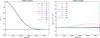 |
Fig. 3 Effective beam window matrix |

Figure 2 shows the same information for an hypothetical LiteBIRD5 like detector (but without half-wave plate modulation) in which we assumed the detector to cover a circle of 45° in radius in one minute, with its spin axis precessing with a period of four days at 50° from the anti-sun direction. As expected for such a scanning strategy, the values of α are pretty uniformly distributed over the range [0,2π], which translates into a low amplitude of the ⟨cos2α⟩ and ⟨sin2α⟩ maps. Even if those maps do not look as smooth as those of Planck, their power spectra peak at fairly low multipole values.
3.2. Arbitrary beams, smooth scanning case
If one assumes that ωs(p) and  vary slowly across the sky, as we just saw in the case of Planck and LiteBIRD – and probably a wider class of orbital and sub-orbital missions – then
  is dominated by low ℓ′ values and one expects ℓ ≃ ℓ′′ because of the triangle relation imposed by the 3J symbols (see Appendix C). If one further assumes Cℓ and bℓ to vary slowly in ℓ, then Eqs. (C.5) and (C.9) can be used to impose s1 + v1 = s2 + v2 = s in Eq. (38) and provide
 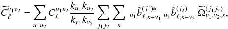 (39)with
 ![Mathematical equation: % subequation 2105 0 \begin{eqnarray} {\tOmega}^{(j_1j_2)}_{v_1,v_2,s} &\equiv & \cpem{j_1,v_1}\cpem{j_2,v_2} \frac{1}{4\pi} \sum_{\ell'm'} {}_{s} {\tomega}^{(j_1) }_{\ell'm'}[v_1] \ {}_{s} {\tomega}^{(j_2)*}_{\ell'm'}[v_2], \label{eq:omega_lm}\\ &=& \cpem{j_1,v_1}\cpem{j_2,v_2} \frac{1}{\npix} \sum_p \tomega_{s}^{(j_1)}[v_1](p)\ \tomega_{s}^{(j_2)*}[v_2](p), \label{eq:omega_pixel}\\ &=& {\tOmega}^{(j_1j_2)*}_{-v_1,-v_2,-s}. \end{eqnarray}](/articles/aa/full_html/2017/02/aa29626-16/aa29626-16-eq136.png) As derived in Appendix E.1, Eq. (39) reduces to a mixing equation relating the observed cross-power spectra to the true ones:
As derived in Appendix E.1, Eq. (39) reduces to a mixing equation relating the observed cross-power spectra to the true ones: 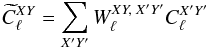 (41)with X,Y,X′,Y′ ∈ { T,E,B }.
In the smooth scanning case representative of past and forthcoming satellite missions, the effect of observing the sky with non-ideal beams is therefore to couple the temperature and polarization power spectra  at the same multipole ℓ through an extended beam window matrix
  , as illustrated in Fig. 3.
3.3. Arbitrary scanning, circular identical beams
If the scanning beams are now assumed to all be circular and identical, the measured  will not depend on the details of the scanning strategy, orientation of the detectors, or relative weights of the detectors. We are indeed exactly in the ideal hypotheses of the map making formalism (Eq. (29)) and get the well known and simple result that the effect of the beam can be factored out.
If one considers detectors with identical circular copolarized beams, and whose actual polarization efficiency was used during the map making:  , such that
 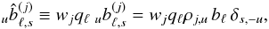 (42)then Eqs. (39) and (40b) feature terms like
 ![Mathematical equation: \hbox{$\sum_{j}\, _{u} \hatb^{(j)*}_{\ell,s-v} \cpem{j,v} \tomega_{s}^{(j)}[v]$}](/articles/aa/full_html/2017/02/aa29626-16/aa29626-16-eq144.png) , which when written in a matrix form, verify the equality
, which when written in a matrix form, verify the equality ![Mathematical equation: \begin{eqnarray} q_\ell b_\ell \sum_{j} w_j \matrixthree { {\tomega_{0 }^{(j)}[0]}} {\cpem{j} {\tomega_{ -2}^{(j)}[0] }} {\cpem{j} {\tomega_{ 2}^{(j)}[0] }} {\cpem{j} {\tomega_{ 2}^{(j)}[2] }} {\cpem{j}^2{\tomega_{0 }^{(j)}[2] }} {\cpem{j}^2{\tomega_{ 4}^{(j)}[2] }} {\cpem{j} {\tomega_{ -2}^{(j)}[-2]}} {\cpem{j}^2{\tomega_{ -4}^{(j)}[-2]}} {\cpem{j}^2{\tomega_{0 }^{(j)}[-2]}} = q_\ell b_\ell \matrixthree {1}{0}{0}{0}{1}{0}{0}{0}{1}, \end{eqnarray}](/articles/aa/full_html/2017/02/aa29626-16/aa29626-16-eq145.png) (43)according to Eq. (B.9). The measured power spectra are then
(43)according to Eq. (B.9). The measured power spectra are then 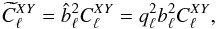 (44)and
  for the Gaussian circular beam introduced in Eq. (23a). Obviously, these very simple results assume that the whole sky is observed. If not, the cut-sky induced ℓ−ℓ and E−B coupling effects mentioned at the end of Sect. 2.4 have to be accounted for, as described, for example, in Chon et al. (2004), Mitra et al. (2009), Grain et al. (2009), and references therein.
3.4. Arbitrary beams, ideal scanning
Let us now consider the case of an ideal scanning of the sky, for which in any pixel p, the number of valid (unflagged) samples is the same for all detectors hj(p) = h(p), and each detector j covers uniformly all possible orientations within that pixel along the duration of the mission. This constitutes the ideal limit aimed at by the scanning strategy illustrated in Fig. 2. The assumption of smooth scanning is then perfectly valid, and details of the calculations can be found in Appendix E.2. We find for instance that the matrix describing how the measured temperature and polarization power spectra are affected by the input TT spectrum reads 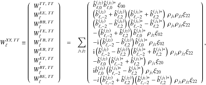 (45)with the normalization factors
  (46)This confirms that in this ideal case, as expected and discussed previously (e.g., Wallis et al. 2014, and references therein), the leakage from temperature to polarization (Eq. (45)) is driven by the beam ellipticity (
 terms) which has the same spin ± 2 as polarization. One also sees that the contamination of the E and B spectra by T are swapped (e.g.,
 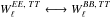 ) when the beams are rotated with respect to the polarimeter direction by 45° (
 ), as shown in Shimon et al. (2008).
3.5. Finite pixel size and sub-pixel effects
As shown in Planck Collaboration VII (2014), in the case of temperature fluctuations, the effect of the finite pixel size is twofold. First, in each pixel, the distance between the nominal pixel center and the center of mass of the observations couples to the local gradient of the Stokes parameters to induce noise terms. Second, there is a smearing effect due to the integration of the signal over the surface of the pixel. Equation (41) then becomes  (47)with
 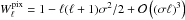 , and
, and  the squared displacement averaged over the hits in the pixels and over the set of considered pixels. As shown in Appendix F, the additive noise term, sourced by the temperature gradient within the pixel, affects both temperature and polarization measurements, with
  and
and  , while the other spectra are much less affected, that is,
  . The sign of this noise term is arbitrary and can be negative when cross-correlating maps with a different sampling of the pixels.
4. Numerical implementation
Numerical implementations of this formalism are performed in three steps, assuming that the individual beam  is already computed for 0 ≤ s ≤ smax + 4 and 0 ≤ ℓ ≤ ℓmax:
- 1.
For each involved detector j, and for 0 ≤ s ≤ smax, one computes the sth complex moment of its direction of polarization in pixel p:
 defined in Eq. (A.3). Since this requires processing the whole scanning data stream, this step can be time consuming. However it has to be computed only once for all cases, independently of the choices made elsewhere on the beam models, calibrations, noise weighting, and other factors. As we shall see below, it may not even be necessary to compute it, or store it, for every sky pixel.
 - 2.
The
computed above are weighted with the assumed inverse noise variance weights wj and polar efficiencies ρj to build the hit matrix H in each pixel, which is then inverted to compute the  , defined in Eq. (A.6). Those are then multiplied together to build the scanning information matrix
  using its pixel space definition (Eq. (40b)). The resulting complex matrix contains 9n1n2(2smax + 1) elements, where n1 and n2 are the number of detectors in each of the two detector assemblies whose cross-spectra are considered. This step can be parallelized to a large extent, and can be dramatically sped up by building this matrix out of a representative subset of pixels. In our comparison to simulations, described in Sect. 5, and performed on HEALPix map with nside = 2048 and
  pixels, we checked that using only Npix/ 64 pixels evenly spread on the sky gave final results almost identical to those of the full calculations.
 Finally, using Eqs. ((E.1)–(41)) we note that
 , so that, for instance, for a given ℓ, the 3x3
  matrix is computed by replacing in Eq. (E.1) its central term Cℓ with its partial derivative, such as
 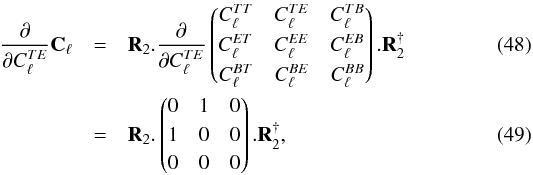 where we assumed in Eq. (49) that, on the sky,
  and generally
  , like for CMB anisotropies. On the other hand, when dealing with arbitrary foregrounds cross-frequency spectra, we would have to assume
  when X′ ≠ Y′, and compute and
  separately. As we shall see in Sect. 6, this final and fastest step is the only one that needs to be repeated in a Monte-Carlo analysis of instrumental errors, and it can be sped up. Indeed, since the input bℓm and output Wℓ are generally very smooth functions of ℓ, it is not necessary to do this calculation for every single ℓ, but rather for a sparse subset of them, for instance regularly interspaced by δℓ. The resulting Wℓ matrix is then B-spline interpolated. In our test cases with θFWHM = 10 to 5′, using δℓ = 10 leads to relative errors on the final product below 10-5 for each ℓ.
In our tests, with smax = 6, ℓmax = 4000, n1 = n2 = 4, and all proposed speed-ups in place, Step 2 took about ten minutes, dominated by IO, while Step 3 took less than a minute on one core of a 3 GHz Intel Xeon CPU. The final product is a set of six (or nine) real matrices , each with 9(ℓmax + 1) elements.
5. Comparison to Planck-HFI simulations
The differential nature of the polarization measurements, in the absence of modulating devices such as rotating half-wave plates, means that any mismatch between the responses of the two (or more) detectors being used will leak a fraction of temperature into polarization. This was observed in Planck, even though pairs of polarized orthogonal detectors observed the sky through the same horn, therefore with almost identical optical beams. Optical mismatches within pairs of detectors were enhanced by residuals of the electronic time response deconvolution which could affect their respective scanning beams differently (Planck Collaboration IV 2014; Planck Collaboration VII 2014). Other sources of mismatch included their different noise levels and thus their respective statistical weight on the maps, which could reach relative differences of up to 80%, and the number of valid samples which could vary by up to 20% between detectors. As seen previously, these detector-specific features can be included in the QuickPol pipeline in order to describe as closely as possible the actual instrument. In this section, we show how we actually did it and how QuickPol compares to full-fledged simulations of Planck-HFI observations.
Noiseless simulations of Planck-HFI observations of a pure CMB sky were run for quadruplets of polarized detectors at three different frequencies (100, 143, and 217 GHz), and identified as 100ds1, 143ds1, and 217ds1 respectively. The input CMB power spectrum  was assumed to contain no primordial tensorial modes, with the traditional
  and
and  . The same mission duration, pointing, polarization orientations (γj) and efficiencies (ρj), flagged samples, and discarded pointing periods (fj) were used as in the actual observations, with computer simulated polarized optical beams for the relevant detectors produced with the GRASP6 physical optics code (Rosset et al. 2007, and references therein) as illustrated on Fig. 4. Data streams were generated with the LevelS simulation pipeline (Reinecke et al. 2006), using the Conviqt code (Prézeau & Reinecke 2010) to perform the convolution of the sky with the beams, including the bℓs for | s | ≤ smax = 14 and ℓ ≤ ℓmax = 4800. Polarized maps of each detector set were produced with the Polkapix destriping code (Tristram et al. 2011), assuming the same noise-based relative weights (wj) as the actual data, and their cross spectra were computed over the whole sky with HEALPix anafast routine to produce the empirical power spectra
  .
.
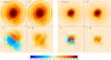 |
Fig. 4 Computer simulated beam maps ( |

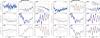 |
Fig. 5 Comparison to simulations for 100ds1x217ds1 (lhs panels) and 143ds1x217ds1 (rhs panels) cross power spectra, for computer simulated beams. In each panel is shown the discrepancy between the actual ℓ(ℓ + 1)Cℓ/ 2π and the one in input, smoothed on Δℓ = 31. Results obtained on simulations with either the full beam model (green curves) or the co-polarized beam model (blue dashes) are to be compared to QuickPol analytical results (red long dashes). In panels where it does not vanish, a small fraction of the input power spectrum is also shown as black dots for comparison. |
The same exercise was reproduced replacing the initial  beam maps with a purely co-polarized beam based on the same , in order to test the validity of the co-polarized assumption in Planck.
Figure 5 shows how the empirical power spectra are different from the input ones, 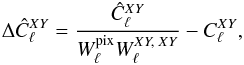 (50)after correction from the pixel and (scalar) beam window functions, and compares those to the QuickPol predictions
 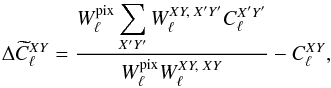 (51)for all nine possible values of XY for the cross-spectra of detector sets 100ds1x217ds1 and 143ds1x217ds1. The results are actually multiplied by the usual ℓ(ℓ + 1)/2π factor, and smoothed on Δℓ = 31. The empirical results are shown both for the full-fledged beam model (green curves) and the purely co-polarized model (blue dashes). One sees that the change, mostly visible in the EE case, is very small, validating the co-polarized beam assumption, at least within the limits of this computer simulated Planck optics. The QuickPol predictions, only shown in the co-polarized case for clarity (long red dashes), agree extremely well with the corresponding numerical simulations. We have checked that this agreement to simulations remains true in the full beam model.
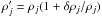
6. Propagation of instrumental uncertainties
We assumed so far the instrument to be non-ideal, but exactly known. In practice, however, the instrument is only known with limited accuracy and the final beam matrix will be affected by at least four types of uncertainties:
-
limited knowledge of the beam angular response, which affects the
 , replacing them with
  while preserving the beam total throughput after calibration (see below)
  . We therefore assume the beam power spectrum Wℓ = ∑ m | bℓm | 2/ (2ℓ + 1) to be the same at ℓ = 0, where the beam throughput is defined, and at ℓ = 1, where the detector gain calibration is usually done using the CMB dipole.
 -
error on the gain calibration of detector j, which translates into
 , with | δcj | ≪ 1,
 -
error on the polar efficiency of detector j, which translates into
 . As discussed in Sect. 2.1, we expect in the case of Planck-HFI a relative uncertainty | δρj/ρj | < 1%.
 -
error on the actual direction of polarization: for each detector j, the direction of polarization measured in a common referential becomes γj− → γj + δγj. In the case of Planck-HFI, Rosset et al. (2010) found the pre-flight measurement of this angle to be dominated by systematic errors of the order of 1° for polarization sensitive bolometers (PSBs). These uncertainties can be larger for spider web bolometers (SWBs), but as we shall see below, the coupling with the low polarization efficiency ρj of those detectors makes them somewhat irrelevant.
All these uncertainties can be inserted in Eq. (E.1) by substituting Eq. (E.4) 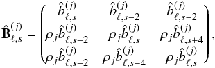 with
with 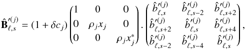 (52)where xj = (1 + δρj/ρj)e2iδγj.
As mentioned in Sect. 3, such substitutions are done in Step 3 of the QuickPol pipeline. A new set of numerical values for the instrument model can therefore be turned rapidly into a beam window matrix (Eq. (41)), allowing, for instance, a Monte-Carlo exploration at the power spectrum level of the instrumental uncertainties.
7. About rotating half-wave plates
In the previous sections we have focused on experiments that rely on the rotation of the full instrument with respect to the sky to have the angular redundancy required to measure the Stokes parameters. An alternative way is to rotate the incoming polarization at the entrance of the instrument while leaving the rest fixed. This is most conveniently achieved with a rotating half-wave plate (rHWP). The rotation is either stepped (POLARBEAR Collaboration 2014) or continuous (Chapman et al. 2014; Essinger-Hileman et al. 2016; Ritacco et al. 2016a). The advantages of this system are numerous, the first of which is the decoupling between the optimization of the scanning strategy in terms of “pure” redundancy and its optimization in terms of “angular” redundancy. It is much easier to control the rotation of a rHWP than of a full instrument and therefore ensure an optimal angular coverage whatever the observation scene is. If the rotation is continuous and fast, typically of the order of 1 Hz, it has the extra advantage of modulating polarization at frequencies larger than the atmospheric and electronics 1 /f noise knee frequency, hence ensuring a natural rejection of these low frequency noises. Furthermore, this allows us to build I, Q, and U maps per detector, without needing to combine different detectors with their associated bandpass mismatch or other differential systematic effects mentioned in the previous sections. Individual detector systematics therefore tend to average out rather than combine to induce leakage between sky components. On the down side, this comes at the price of moving a piece of hardware in the instrument and all its associated systematic effects, starting with a signal that is synchronous with the rHWP rotation as observed in Johnson et al. (2007), Chapman et al. (2014), and Ritacco et al. (2016b).
Such trade-offs are being investigated by current experiments using rHWPs and will certainly be studied in more details in preparation of future CMB orbital and sub-orbital missions, such as CMB-S4 network (CMB-S4 Collaboration 2016). We here briefly comment on how the addition of a rHWP to an instrument can be coped with in QuickPol.
The Jones matrix of a HWP (which shifts the y-axis electric field by a half period) rotated by an angle ψ is (O’Dea et al. 2007) 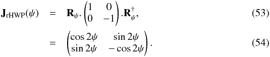 If a rotating HWP is installed at the entrance of the optical system, the Jones matrix of the system becomes
  , and the signal observed in the presence of arbitrary beams (Eq. (8)) becomes (after dropping the circular polarization V terms)
 ![Mathematical equation: \begin{eqnarray} {\rm d}(\alpha,\psi) = \frac{1}{2} \int {\rm d}\vecr \left[ \bI (\alpha, \psi, \vecr)T(\vecr) +\bQ (\alpha, \psi, \vecr)Q(\vecr) +\bU (\alpha, \psi, \vecr)U(\vecr) \right], \label{eq:datastream_beam_rHWP} \end{eqnarray}](/articles/aa/full_html/2017/02/aa29626-16/aa29626-16-eq239.png) (55)with
(55)with 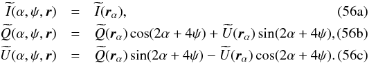 These new beams can then be passed to Eq. (30) and propagated through the rest of QuickPol. Together with Eq. (9), we see that, if ψ is correctly chosen, the modulation of Q and U, by 2α + 4ψ, is now clearly different from that of T which depends only on α via rα, even for non-circular beams. The leakages from temperature to polarization are therefore expected to be much smaller than when the polarization modulation is performed only by a rotation of the whole instrument, and O’Dea et al. (2007) showed, that even for non-ideal rHWP, the induced systematic effects are limited to polarization cross-talks without temperature to polarization leakage.
As previously mentioned, specific systematic effects such as the rotation synchronous signal must be treated with care. Once such time domain systematic effects are identified and modeled, they, together with realistic optical properties of the instrument, can be integrated in the QuickPol formalism in order to be taken into account, quantified, and/or marginalized over at the power spectrum level.
8. Conclusions
Polarization measurements are mostly obtained by differencing observations by different detectors. Mismatch in their optical beams, time responses, bandpasses, and so on induces systematic effects, for example, temperature to polarization leakage. The QuickPol formalism allows us to compute accurately and efficiently the induced cross-talk between temperature and polarization power spectra. It also provides a fast and easy way to propagate instrumental modeling uncertainties down to the final angular power spectra and is thus a powerful tool to simulate observations and to help with the design and specifications of future experiments, such as acceptable beam distortions, polarization modulation optimization, and observation redundancy. It can cope with time varying instrumental parameters, realistic sample flagging, and rejection. The method was validated through comparison to numerical simulations of realistic Planck observations. The hypotheses required on the instrument and survey, described in Sects. 2 and 3, are extremely general and apply to Planck and to forthcoming CMB experiments such as PIXIE, LiteBIRD, COrE, and others. Contrary to Monte-Carlo based methods, such as FEBeCoP, the impact of the beam related imperfections on the measured power spectra are obtained without having to assume any prior knowledge of the sky power spectra.
Of course, the beam matrices provided by QuickPol can be used in the cosmological analysis of a CMB survey. Indeed, the sky power spectra can be modeled as functions of cosmological parameters { θC }, foreground modeling { θF }, and nuisance parameters { θn }. These  can then be generated, multiplied with the beam matrices
  for the set of detectors being analyzed, and compared to the measured
  in a maximum likelihood sense, in the presence of instrumental noise. The parameters { θC } , { θF } , { θn } can be iterated or integrated upon, with statistical priors, until a posterior distribution is built. In this kind of forward approach, it is not necessary to correct the observations from possibly singular transfer functions, nor to back-propagate the noise. At least some of the instrumental uncertainties { θI } affecting the effective beam via
  could be included in the overall analysis, and marginalized over, thanks to the fast calculation times by QuickPol of the impact of changes in the gain calibrations, polarization angles, and efficiencies, as discussed in Sect. 6. While QuickPol has been originally developed and tested in the case of experiments without a rotating half-wave plate, it is straightforward to add one to the current pipeline and assess its impact on the aforementioned systematics. Specific additional effects such as a HWP rotation synchronous signal or the effect of a tilted HWP are expected to show up in real experiments. As long as these can be physically modeled, they can be inserted in QuickPol as well.
Wilkinson microwave anisotropy probe: http://map.gfsc.nasa.gov.
Although it is important when trying to disentangle sky signals with different electromagnetic spectra (Planck Collaboration VI 2014), the finite bandwidth of the actual detectors only plays a minor role in the problem considered here, and will be ignored in this paper.
TICRA: http://www.ticra.com.
Acknowledgments
Thank you to the Planck collaboration, and in particular to D. Hanson, K. Benabed, and F. R. Bouchet for fruitful discussions. Some results presented here were obtained with the HEALPix library.
References
- Armitage-Caplan, C., & Wandelt, B. D. 2009, ApJS, 181, 533 [NASA ADS] [CrossRef] [Google Scholar]
- Bennett, C. L., Larson, D., Weiland, J. L., et al. 2013, ApJS, 208, 20 [Google Scholar]
- Bunn, E. F., Zaldarriaga, M., Tegmark, M., & de Oliveira-Costa, A. 2003, Phys. Rev. D, 67, 023501 [NASA ADS] [CrossRef] [Google Scholar]
- Challinor, A., Fosalba, P., Mortlock, D., et al. 2000, Phys. Rev. D, 62, 123002 [NASA ADS] [CrossRef] [Google Scholar]
- Chapman, D., Aboobaker, A. M., Ade, P., et al. 2014, Am. Astron. Soc. Meet. Abstr., 223, 407.03 [Google Scholar]
- Chon, G., Challinor, A., Prunet, S., Hivon, E., & Szapudi, I. 2004,MNRAS, 350, 914 [Google Scholar]
- CMB-S4 Collaboration 2016, ArXiv e-prints [arXiv:1610.02743] [Google Scholar]
- Edmonds, A. R. 1957, Angular Momentum in Quantum Mechanics (Princeton University Press) [Google Scholar]
- Essinger-Hileman, T., Kusaka, A., Appel, J. W., et al. 2016, Rev. Sci. Inst., 87, 094503 [Google Scholar]
- Fosalba, P., Doré, O., & Bouchet, F. R. 2002, Phys. Rev. D, 65, 063003 [NASA ADS] [CrossRef] [Google Scholar]
- Górski, K. M., Hivon, E., Banday, A. J., et al. 2005, ApJ, 622, 759 [NASA ADS] [CrossRef] [Google Scholar]
- Grain, J., Tristram, M., & Stompor, R. 2009, Phys. Rev. D, 79, 123515 [Google Scholar]
- Hansen, F. K., & Górski, K. M. 2003, MNRAS, 343, 559 [NASA ADS] [CrossRef] [Google Scholar]
- Hanson, D., Lewis, A., & Challinor, A. 2010, Phys. Rev. D, 81, 103003 [NASA ADS] [CrossRef] [Google Scholar]
- Hinshaw, G., Nolta, M. R., Bennett, C. L., et al. 2007, ApJS, 170, 288 [NASA ADS] [CrossRef] [Google Scholar]
- Hivon, E., Górski, K. M., Netterfield, C. B., et al. 2002, ApJ, 567, 2 [NASA ADS] [CrossRef] [Google Scholar]
- Hu, W. 2000, Phys. Rev. D, 62, 043007 [NASA ADS] [CrossRef] [Google Scholar]
- Hu, W., Hedman, M. M., & Zaldarriaga, M. 2003, Phys. Rev. D, 67, 043004 [NASA ADS] [CrossRef] [Google Scholar]
- Johnson, B. R., Collins, J., Abroe, M. E., et al. 2007, ApJ, 665, 42 [NASA ADS] [CrossRef] [Google Scholar]
- Keihänen, E., & Reinecke, M. 2012, A&A, 548, A110 [NASA ADS] [CrossRef] [EDP Sciences] [Google Scholar]
- Keihänen, E., Kiiveri, K., Kurki-Suonio, H., & Reinecke, M. 2016, ArXiv e-prints [arXiv:1610.00962] [Google Scholar]
- Leahy, J. P., Bersanelli, M., D’Arcangelo, O., et al. 2010, A&A, 520, A8 [NASA ADS] [CrossRef] [EDP Sciences] [Google Scholar]
- Lewis, A., & Challinor, A. 2006, Phys. Rep., 429, 1 [Google Scholar]
- Miller, N. J., Shimon, M., & Keating, B. G. 2009a, Phys. Rev. D, 79, 063008 [NASA ADS] [CrossRef] [Google Scholar]
- Miller, N. J., Shimon, M., & Keating, B. G. 2009b, Phys. Rev. D, 79, 103002 [NASA ADS] [CrossRef] [Google Scholar]
- Mitra, S., Sengupta, A. S., & Souradeep, T. 2004, Phys. Rev. D, 70, 103002 [NASA ADS] [CrossRef] [Google Scholar]
- Mitra, S., Sengupta, A. S., Ray, S., Saha, R., & Souradeep, T. 2009, MNRAS, 394, 1419 [NASA ADS] [CrossRef] [Google Scholar]
- Mitra, S., Rocha, G., Górski, K. M., et al. 2011, ApJS, 193, 5 [NASA ADS] [CrossRef] [Google Scholar]
- O’Dea, D., Challinor, A., & Johnson, B. R. 2007, MNRAS, 376, 1767 [NASA ADS] [CrossRef] [Google Scholar]
- Page, L., Hinshaw, G., Komatsu, E., et al. 2007, ApJS, 170, 335 [NASA ADS] [CrossRef] [Google Scholar]
- Pant, N., Das, S., Rotti, A., Mitra, S., & Souradeep, T. 2016, J. Cosmol. Astropart. Phys., 3, 035 [NASA ADS] [CrossRef] [Google Scholar]
- Planck Collaboration IV. 2014, A&A, 571, A4 [NASA ADS] [CrossRef] [EDP Sciences] [Google Scholar]
- Planck Collaboration VI. 2014, A&A, 571, A6 [NASA ADS] [CrossRef] [EDP Sciences] [Google Scholar]
- Planck Collaboration VII. 2014, A&A, 571, A7 [NASA ADS] [CrossRef] [EDP Sciences] [Google Scholar]
- Planck Collaboration VIII. 2014, A&A, 571, A8 [NASA ADS] [CrossRef] [EDP Sciences] [Google Scholar]
- Planck Collaboration XVII. 2014, A&A, 571, A17 [NASA ADS] [CrossRef] [EDP Sciences] [Google Scholar]
- Planck Collaboration VII. 2016, A&A, 594, A7 [NASA ADS] [CrossRef] [EDP Sciences] [Google Scholar]
- Planck Collaboration XI. 2016, A&A, 594, A11 [NASA ADS] [CrossRef] [EDP Sciences] [Google Scholar]
- Polarbear Collaboration 2014, ApJ, 794, 171 [NASA ADS] [CrossRef] [Google Scholar]
- Prézeau, G., & Reinecke, M. 2010, ApJS, 190, 267 [NASA ADS] [CrossRef] [Google Scholar]
- Ramamonjisoa, F. A., Ray, S., Mitra, S., & Souradeep, T. 2013, ArXiv e-prints [arXiv:1309.4784] [Google Scholar]
- Rathaus, B., & Kovetz, E. D. 2014, MNRAS, 443, 750 [NASA ADS] [CrossRef] [Google Scholar]
- Reinecke, M., Dolag, K., Hell, R., Bartelmann, M., & Enßlin, T. A. 2006, A&A, 445, 373 [NASA ADS] [CrossRef] [EDP Sciences] [Google Scholar]
- Ritacco, A., Adam, R., Adane, A., et al. 2016a, ArXiv e-prints [arXiv:1602.01605] [Google Scholar]
- Ritacco, A., Ponthieu, N., Catalano, A., et al. 2016b, ArXiv e-prints [arXiv:1609.02042] [Google Scholar]
- Rosset, C., Yurchenko, V., Delabrouille, J., et al. 2007, A&A, 464, 405 [NASA ADS] [CrossRef] [EDP Sciences] [Google Scholar]
- Rosset, C., Tristram, M., Ponthieu, N., et al. 2010, A&A, 520, A13 [NASA ADS] [CrossRef] [EDP Sciences] [Google Scholar]
- Shimon, M., Keating, B., Ponthieu, N., & Hivon, E. 2008, Phys. Rev. D, 77, 83003 [NASA ADS] [CrossRef] [Google Scholar]
- Smith, K. M., Zahn, O., & Doré, O. 2007, Phys. Rev. D, 76, 043510 [NASA ADS] [CrossRef] [Google Scholar]
- Souradeep, T., & Ratra, B. 2001, ApJ, 560, 28 [NASA ADS] [CrossRef] [Google Scholar]
- Tristram, M., Macías-Pérez, J. F., Renault, C., & Hamilton, J.-C. 2004, Phys. Rev. D, 69, 123008 [NASA ADS] [CrossRef] [Google Scholar]
- Tristram, M., Filliard, C., Perdereau, O., et al. 2011, A&A, 534, A88 [NASA ADS] [CrossRef] [EDP Sciences] [Google Scholar]
- Wallis, C. G. R., Brown, M. L., Battye, R. A., Pisano, G., & Lamagna, L. 2014, MNRAS, 442, 1963 [NASA ADS] [CrossRef] [Google Scholar]
- Wallis, C. G. R., Bonaldi, A., Brown, M. L., & Battye, R. A. 2015, MNRAS, 453, 2058 [NASA ADS] [CrossRef] [Google Scholar]
- Zaldarriaga, M., & Seljak, U. 1997, Phys. Rev. D, 55, 1830 [Google Scholar]
Appendix A: Projection of maps on spherical harmonics
Here we give more details on the steps required to go from Eq. (35) to Eq. (38). Let us recall Eq. (35) and explain it further:
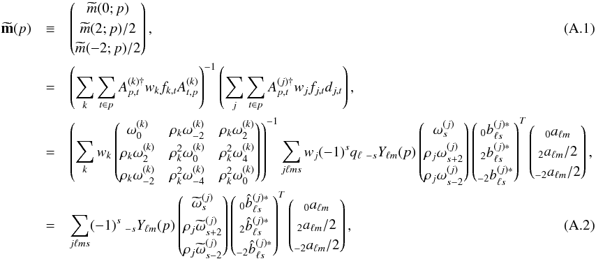 where we introduced the sth complex moment of the direction of polarization for detector j,
 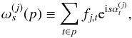 (A.3)the hit matrix H defined for (u,v) ∈ { 0,2,−2 } 2 as
 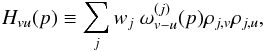 (A.4)with
 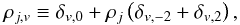 (A.5)the hit normalized moments
 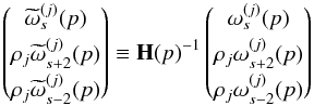 (A.6)which are described in Appendix B, and finally the inverse noise variance weighted beam spherical harmonics (SH) coefficients
 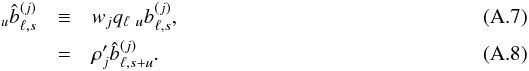 Since the solution of Eq. (33) remains the same when all the noise covariances are rescaled simultaneously by an arbitrary factor a: Nj− → aNj, one can also rescale the weights wj appearing in Eqs (A.4) and (A.7), with for instance wj− → wj/ ∑ kwk without altering the final result.
The components of the observed polarized map are then 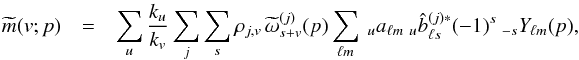 (A.9)with
  (A.10)After expansion of the hit normalized moments (Eq. (A.6)) in spherical harmonics:
 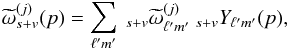 (A.11)the polarized map reads
  (A.12)and the SH coefficients of spin x of map
  are, for pixels of area Ωp,
 ![Mathematical equation: \appendix \setcounter{section}{1} \begin{eqnarray} \ _x \tm_{\ell''m''}(v) &\equiv& \sum_p \Omega_p \tm(v;p)\ _{x}Y^*_{\ell''m''}(p) = \int \dd\vecr\ \tm(v;\vecr)\ _{x}Y^*_{\ell''m''}(\vecr) \\ &=& \sum_u \frac{k_{u}}{k_{v}} \sum_j \sum_{\ell ms \ell'm'} (-1)^s \ _u a_{\ell m} \ _u \hatb^{(j)*}_{\ell s}\, \cpem{j,v} \ _{s+v}\tomega^{(j)}_{\ell'm'} \int \dd \vecr \ _{-s}Y_{\ell m}(\vecr) \ _{s+v} Y_{\ell'm'}(\vecr) \ _x Y^*_{\ell''m''}(\vecr) \nonumber \\ &=& \sum_u \frac{k_{u}}{k_{v}} \sum_{j \ell m s \ell' m'} \ _u a_{\ell m} \ _u \hatb^{(j)*}_{\ell s}\, \cpem{j,v} \ _{s+v}\tomega^{(j)}_{\ell'm'} (-1)^{s+x+m''+\ell+\ell'+\ell''} \left[\frac{(2\ell+1)(2\ell'+1)(2\ell''+1)}{4\pi}\right]^{1/2} \nonumber\\ &&\quad\times \wjjj{\ell}{\ell'}{\ell''}{m}{m'}{-m''} \wjjj{\ell}{\ell'}{\ell''}{-s}{s+v}{-x} \label{eq:map_SH} \end{eqnarray}](/articles/aa/full_html/2017/02/aa29626-16/aa29626-16-eq268.png) which are only non-zero when x = v. The cross power spectrum of spin v1 and v2 maps is then given by Eq. (38).
which are only non-zero when x = v. The cross power spectrum of spin v1 and v2 maps is then given by Eq. (38).
Appendix B: Hit matrix
Introducing, for detector j, 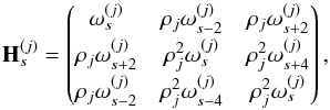 (B.1)the Hermitian hit matrix for a weighted combination of detectors is
 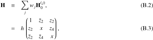 with h,x real and z2,z4 complex numbers, and has for inverse
 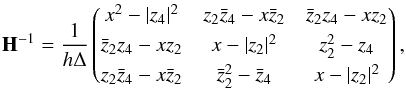 (B.4)with
  (B.5)In Eq. (A.6) we defined
 ![Mathematical equation: \appendix \setcounter{section}{2} \begin{equation} \vectorthree { \tomega_{s}^{(j)}[0]} {\cpem{j}\tomega_{s+2}^{(j)}[2] } {\cpem{j}\tomega_{s-2}^{(j)}[-2]} \equiv \matH^{-1} \vectorthree { \omega_{s }^{(j)}} {\cpem{j} \omega_{s+2}^{(j)}} {\cpem{j} \omega_{s-2}^{(j)}} \end{equation}](/articles/aa/full_html/2017/02/aa29626-16/aa29626-16-eq276.png) (B.6)for any value of s, which provides
(B.6)for any value of s, which provides ![Mathematical equation: \appendix \setcounter{section}{2} \begin{equation} \vectorthree { \tomega_{s}^{(j)}[0]} {\cpem{j}\tomega_{s}^{(j)}[2]} {\cpem{j}\tomega_{s}^{(j)}[-2]} = \frac{1}{h\Delta} \vectorthree { (x^2-\rhob^2)\, \omega_{s}^{(j)} + (\zab-x\cza) \,\cpem{j}\,\omega_{s+2}^{(j)} + (\czab-x\za) \,\cpem{j}\,\omega_{s-2}^{(j)} } { (x-\rhoa^2) \,\cpem{j}\,\omega_{s}^{(j)} + (\czab-x\za)\, \,\omega_{s-2}^{(j)} + (\za^2-\zb) \,\cpem{j}\,\omega_{s-4}^{(j)} } { (x-\rhoa^2) \,\cpem{j}\,\omega_{s}^{(j)} + (\zab-x\cza) \, \,\omega_{s+2}^{(j)} + (\cza^2-\czb)\,\cpem{j}\,\omega_{s+4}^{(j)} }, \end{equation}](/articles/aa/full_html/2017/02/aa29626-16/aa29626-16-eq277.png) (B.7)so that
(B.7)so that  is of spin s, provided z2 and z4 are of spin 2 and 4 respectively. Since
  , we get
 ![Mathematical equation: \hbox{$\tomega_{s}^{(j)*}[2] = \tomega_{-s}^{(j)}[-2]$}](/articles/aa/full_html/2017/02/aa29626-16/aa29626-16-eq282.png) .
.
By definition, ![Mathematical equation: \appendix \setcounter{section}{2} \begin{equation} \matrixthree { {\tomega_{s }^{(j)}[0]}} {\cpem{j} {\tomega_{s-2}^{(j)}[0] }} {\cpem{j} {\tomega_{s+2}^{(j)}[0] }} {\cpem{j} {\tomega_{s+2}^{(j)}[2] }} {\cpem{j}^2{\tomega_{s }^{(j)}[2] }} {\cpem{j}^2{\tomega_{s+4}^{(j)}[2] }} {\cpem{j} {\tomega_{s-2}^{(j)}[-2]}} {\cpem{j}^2{\tomega_{s-4}^{(j)}[-2]}} {\cpem{j}^2{\tomega_{s }^{(j)}[-2]}} = \matH^{-1}. \matH_{s}^{(j)} \end{equation}](/articles/aa/full_html/2017/02/aa29626-16/aa29626-16-eq283.png) (B.8)so that
(B.8)so that ![Mathematical equation: \appendix \setcounter{section}{2} \begin{equation} \sum_j w_j \matrixthree { {\tomega_{0 }^{(j)}[0]}} {\cpem{j} {\tomega_{ -2}^{(j)}[0] }} {\cpem{j} {\tomega_{ 2}^{(j)}[0] }} {\cpem{j} {\tomega_{ 2}^{(j)}[2] }} {\cpem{j}^2{\tomega_{0 }^{(j)}[2] }} {\cpem{j}^2{\tomega_{ 4}^{(j)}[2] }} {\cpem{j} {\tomega_{ -2}^{(j)}[-2]}} {\cpem{j}^2{\tomega_{ -4}^{(j)}[-2]}} {\cpem{j}^2{\tomega_{0 }^{(j)}[-2]}} = \matrixthree {1}{0}{0}{0}{1}{0}{0}{0}{1}. \label{eq:omega0_identity} \end{equation}](/articles/aa/full_html/2017/02/aa29626-16/aa29626-16-eq284.png) (B.9)
(B.9)
Appendix C: Wigner 3J symbols
The Wigner 3J symbols describe the coupling between different spin weighted spherical harmonics at the same location:  (C.1)and the symbol
  is non-zero only when, | mi | ≤ ℓi for i = 1,2,3, m1 + m2 + m3 = 0 and
  (C.2)They obey the relations
  (C.3)and
  (C.4)Their standard orthogonality relations are
  (C.5)and
  (C.6)where δ(ℓ1,ℓ2,ℓ3) = 1 when ℓ1,ℓ2,ℓ3 obey the triangle relation of Eq. (C.2) and vanishes otherwise.
For ℓ1 ≪ ℓ2,ℓ3 (Edmonds 1957, Eq. (A2.1))  (C.7)where d is the Wigner rotation matrix and cosθ = 2m2/ (2ℓ2 + 1). As a consequence, for | m2 | ≪ ℓ2
 (C.8)and an approximate orthogonality relation can therefore be written, for ℓ1, | m1 | , | m2 | ≪ ℓ2,ℓ3
 (C.9)
(C.9)
Appendix D: Spin weighted power spectra
Since a complex field of spin s can be written as Cs = Rs + iIs where Rs and Is are real, with  (D.1)and, with the Condon-Shortley phase convention
  then
then  (D.2)When s = 2, one defines
 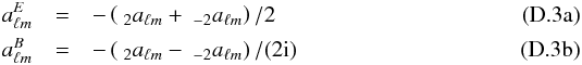 such that
  , with X = E,B, and
 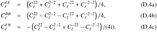 When s = 1, one defines
 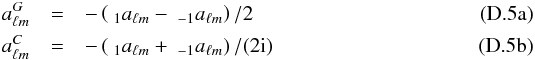 such that , with X = G,C, and
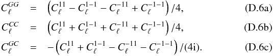
Appendix E: Window matrices W
Appendix E.1: Arbitrary beams, smooth scanning case
Let us come back to Eqs. (39) and (40). These can be cast in a more compact matrix form ![Mathematical equation: \appendix \setcounter{section}{5} \begin{eqnarray} \widetilde{\matC}_{\ell} = \sum_{j_1j_2}\sum_s \left\{ \left[\matD^{-1}. \hat{\matB}^{(j_1)\dagger}_{\ell,s}. \matD\ . \ \matC_{\ell} \ .\ \matD. \hat{\matB}^{(j_2)}_{\ell,s}. \matD^{-1} \right] * \widetilde{\bf \Omega}^{(j_1j_2)}_s \right\} \label{eq:main} \end{eqnarray}](/articles/aa/full_html/2017/02/aa29626-16/aa29626-16-eq321.png) (E.1)where
(E.1)where 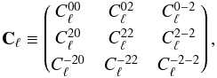 (E.2)
(E.2) (E.3)
(E.3)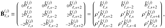 (E.4)and X ∗ Y denotes the elementwise product (also known as Hadamard or Schur product) of arrays X and Y. Noting that
 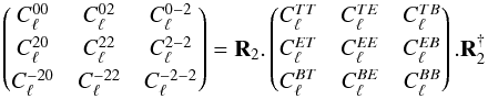 (E.5)where R2 was introduced in Eq. (18), which leads to Eq. (41) that we recall here for convenience:
 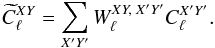 (E.6)Introducing the short-hand
  (E.7)describing the coupled moments of the polarized detectors j1 and j2 orientation, and assuming in Eq. (E.4) the beams to be perfectly co-polarized, with polar efficiencies
  , one gets, for XY = TT,EE,BB,TE,TB,EB,ET,BT,BE:
 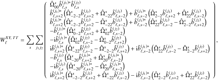 (E.8a)which is illustrated in Fig. 3;
 ![Mathematical equation: \appendix \setcounter{section}{5} % subequation 4741 1 \begin{eqnarray} W_{\ell}^{XY,\; EE} = \sum_s \sum_{j_1j_2} \frac{\cpei{j_1} \cpei{j_2}}{4} \left( \begin{array}{l} \pO_{00} \left( \hatb_{\ell,s-2}^{(j_1)*}+\hatb_{\ell,s+2}^{(j_1)*}\right) \left( \hatb_{\ell,s-2}^{(j_2)} +\hatb_{\ell,s+2}^{(j_2)} \right)\\[1mm] \hatb_{\ell,s}^{(j_1)*} \left[\hatb_{\ell,s}^{(j_2)} \left( \pO_{-2-2}+\pO_{-22}+\pO_{2-2}+\pO_{22} \right) +\hatb_{\ell,s+4}^{(j_2)} \left( \pO_{-2-2}+\pO_{2-2} \right) +\hatb_{\ell,s-4}^{(j_2)} \left( \pO_{-22}+\pO_{22} \right)\right] \\[1mm] \quad\quad +\hatb_{\ell,s+4}^{(j_1)*} \left[\hatb_{\ell,s}^{(j_2)} \left( \pO_{-2-2}+\pO_{-22} \right) +\pO_{-2-2} \hatb_{\ell,s+4}^{(j_2)}+\pO_{-22} \hatb_{\ell,s-4}^{(j_2)} \right] \\[1mm] \end{array} \right),~~~~~~~~~~~~~~~~~~~~~~~~~ \label{eq:wl_xyEE} \end{eqnarray}](/articles/aa/full_html/2017/02/aa29626-16/aa29626-16-eq337.png) (E.8b)
(E.8b)![Mathematical equation: \appendix \setcounter{section}{5} % subequation 4741 2 \begin{eqnarray} W_{\ell}^{XY,\; TE} = \sum_s \sum_{j_1j_2} \frac{\cpei{j_2}}{2} \left( \begin{array}{l} -\pO_{00} \hatb_{\ell,s}^{(j_1)*} \left( \hatb_{\ell,s-2}^{(j_2)}+\hatb_{\ell,s+2}^{(j_2)} \right) \\[1mm] -\hatb_{\ell,s+2}^{(j_1)*} \left[\hatb_{\ell,s}^{(j_2)} \left( \pO_{-2-2}+\pO_{-22} \right) +\pO_{-2-2} \hatb_{\ell,s+4}^{(j_2)}+\pO_{-22} \hatb_{\ell,s-4}^{(j_2)} \right] \\[1mm] \quad\quad -\hatb_{\ell,s-2}^{(j_1)*} \left[\hatb_{\ell,s}^{(j_2)} \left( \pO_{2-2}+\pO_{22} \right) +\pO_{2-2} \hatb_{\ell,s+4}^{(j_2)}+\pO_{22} \hatb_{\ell,s-4}^{(j_2)} \right] \\[1mm] -\hatb_{\ell,s+2}^{(j_1)*} \left[\hatb_{\ell,s}^{(j_2)} \left( \pO_{-2-2}-\pO_{-22} \right) +\pO_{-2-2} \hatb_{\ell,s+4}^{(j_2)}-\pO_{-22} \hatb_{\ell,s-4}^{(j_2)} \right] \\[1mm] \end{array} \right).~~~~~~~~~~~~~~~~~~~~~~~~~ \label{eq:wl_xyTE} \end{eqnarray}](/articles/aa/full_html/2017/02/aa29626-16/aa29626-16-eq338.png) (E.8c)Since, by definition (Eqs. (A.7) and (E.7)),
(E.8c)Since, by definition (Eqs. (A.7) and (E.7)),  and
and  , one can check that each term of is real, as expected.
Appendix E.2: Arbitrary beams, ideal scanning
In the case of ideal scanning described in Sect. 3.4, one gets  , so that the hit matrix is diagonal:
 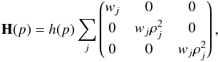 (E.9)and the orientation moments
 ![Mathematical equation: \appendix \setcounter{section}{5} \begin{eqnarray} \tomega^{(j)}_s[0] = \delta_{s,0} \left(\sum_k w_k \right)^{-1}, ~~ \tomega^{(j)}_s[\pm2] = \delta_{s,0} \left(\sum_k w_k\cpem{k}^2\right)^{-1}, \end{eqnarray}](/articles/aa/full_html/2017/02/aa29626-16/aa29626-16-eq343.png) (E.10)are such that
(E.10)are such that 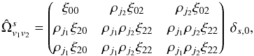 (E.11)with
  (E.12)One then obtains the beam matrices
 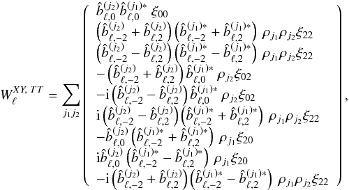 (E.13a)
![Mathematical equation: \appendix \setcounter{section}{5} % subequation 4894 1 \begin{eqnarray} W_{\ell}^{XY,\; EE} = \sum_{j_1j_2} \frac{\cpei{j_1} \cpei{j_2}}{4} \left( \begin{array}{l} \left( \hatb_{\ell,-2}^{(j_2)}+\hatb_{\ell,2}^{(j_2)} \right) \left(\hatb_{\ell,-2}^{(j_1)*}+\hatb_{\ell,2}^{(j_1)*}\right) {\ \myxi_{00}} \\[1mm] \left( \hatb_{\ell,-4}^{(j_2)}+2 \hatb_{\ell,0}^{(j_2)}+\hatb_{\ell,4}^{(j_2)} \right) \left(\hatb_{\ell,-4}^{(j_1)*}+2 \hatb_{\ell,0}^{(j_1)*}+\hatb_{\ell,4}^{(j_1)*}\right) {\ \cpem{j_1}\cpem{j_2}\myxi_{22}} \\[1mm] \left( \hatb_{\ell,-4}^{(j_2)}-\hatb_{\ell,4}^{(j_2)} \right) \left(\hatb_{\ell,-4}^{(j_1)*}-\hatb_{\ell,4}^{(j_1)*}\right) {\ \cpem{j_1}\cpem{j_2}\myxi_{22}} \\[1mm] -\left( \hatb_{\ell,-4}^{(j_2)}+2 \hatb_{\ell,0}^{(j_2)}+\hatb_{\ell,4}^{(j_2)} \right) \left(\hatb_{\ell,-2}^{(j_1)*}+\hatb_{\ell,2}^{(j_1)*}\right) {\ \cpem{j_2}\myxi_{02}} \\[1mm] \end{array} \right),~~~~~~~~~~~~~~~~~~~ \label{eq:wl_xyEE_is} \end{eqnarray}](/articles/aa/full_html/2017/02/aa29626-16/aa29626-16-eq347.png) (E.13b)
(E.13b)![Mathematical equation: \appendix \setcounter{section}{5} % subequation 4894 2 \begin{eqnarray} W_{\ell}^{XY,\; TE} = \sum_{j_1j_2} \frac{\cpei{j_2}}{2} \left( \begin{array}{l} -\left( \hatb_{\ell,-2}^{(j_2)}+\hatb_{\ell,2}^{(j_2)} \right) \hatb_{\ell,0}^{(j_1)*} {\ \myxi_{00}} \\[1mm] -\left( \hatb_{\ell,-4}^{(j_2)}+2 \hatb_{\ell,0}^{(j_2)}+\hatb_{\ell,4}^{(j_2)} \right) \left(\hatb_{\ell,-2}^{(j_1)*}+\hatb_{\ell,2}^{(j_1)*}\right) {\ \cpem{j_1}\cpem{j_2}\myxi_{22}} \\[1mm] -\left( \hatb_{\ell,-4}^{(j_2)}-\hatb_{\ell,4}^{(j_2)} \right) \left(\hatb_{\ell,-2}^{(j_1)*}-\hatb_{\ell,2}^{(j_1)*}\right) {\ \cpem{j_1}\cpem{j_2}\myxi_{22}} \\[1mm] \left( \hatb_{\ell,-4}^{(j_2)}+2 \hatb_{\ell,0}^{(j_2)}+\hatb_{\ell,4}^{(j_2)} \right) \hatb_{\ell,0}^{(j_1)*} {\ \cpem{j_2}\myxi_{02}} \\[1mm] {\rm i} \left( \hatb_{\ell,-4}^{(j_2)}-\hatb_{\ell,4}^{(j_2)} \right) \hatb_{\ell,0}^{(j_1)*} {\ \cpem{j_2}\myxi_{02}} \\[1mm] \end{array} \right).~~~~~~~~~~~~~~~~~~~ \label{eq:wl_xyTE_is} \end{eqnarray}](/articles/aa/full_html/2017/02/aa29626-16/aa29626-16-eq348.png) (E.13c)The implications of Eq. (E.13) are discussed in Sect. 3.4.
(E.13c)The implications of Eq. (E.13) are discussed in Sect. 3.4.
Appendix F: Finite pixel size
Introducing the spin raising and lowering differential operators applied to a function f of spin s, (Zaldarriaga & Seljak 1997; Bunn et al. 2003, and references therein) ![Mathematical equation: \appendix \setcounter{section}{6} \begin{eqnarray} \dbar f &=& - \sin^{s} \theta \left(\frac{\partial}{\partial \theta} + \frac{i}{\sin\theta}\frac{\partial}{\partial \varphi} \right) \left[\sin^{-s}\theta\ f \right] \quad = s \cot\theta\ f - \frac{\partial f}{\partial \theta} - \frac{i}{\sin\theta}\frac{\partial f}{\partial \varphi} ~~~~~~~~~~~~~~~~~~~~\\ \bardbar f &=& - \sin^{-s} \theta \left(\frac{\partial}{\partial \theta} - \frac{i}{\sin\theta}\frac{\partial}{\partial \varphi} \right) \left[\sin^{s}\theta\ f \right] \quad = -s \cot\theta\ f - \frac{\partial f}{\partial \theta} + \frac{i}{\sin\theta}\frac{\partial f}{\partial \varphi}~~~~~~~~~~~~~~~~~~~~ \end{eqnarray}](/articles/aa/full_html/2017/02/aa29626-16/aa29626-16-eq350.png) the spin weighed spherical harmonics are defined as
the spin weighed spherical harmonics are defined as 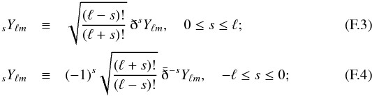 such that
  with
with  .
.
As noticed in Planck Collaboration VII (2014) and Planck Collaboration XVII (2014), the formalism of subpixel effect is very close to the one of gravitational lensing described in Hu (2000) and Lewis & Challinor (2006).
For r = (1,θ,ϕ) = er and dr = (0,dθ,dϕ) = dθeθ + sinθdϕeϕ, 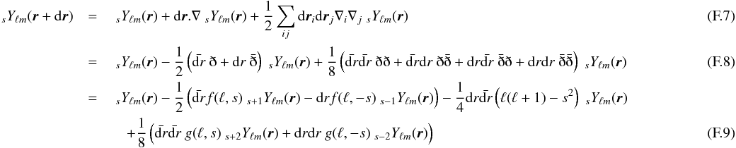 with dr = dr.(eθ + ieϕ) = dθ + isinθdϕ,
  and g(ℓ,s) = f(ℓ,s)f(ℓ,s + 1).
Identifying dr to the position of a measurement relative to the nominal center r of the pixel to which it is attributed, this expansion of  can be injected into Eqs. (28) and (A.14). Assuming dr to be uncorrelated with the orientation of the detector, two extra terms, both quadratic in dr, will appear in the final power spectra.
The first term involves the scalar product of the gradient of the signal in the pixel, assumed to be totally dominated by the temperature, with the weighted sum of dr over all samples in that pixel. Introducing 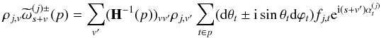 (F.10)which is of spin s + v ± 1 and such that
  , one finds
 ![Mathematical equation: \appendix \setcounter{section}{6} \begin{eqnarray} \Delta \pC^{v_1v_2}_{\ell''} &= & \frac{1}{k_{v_1}k_{v_2}} \sum_{s_1 s_2} (-1)^{s_1+s_2} \sum_{j_1 j_2 \ell} \ell(\ell+1) \frac{2\ell+1}{4\pi} C^{TT}_{\ell} \hatb^{(j_1)*}_{\ell s_1} \, \hatb^{(j_2)}_{\ell s_2} \nonumber \\ &&\ \times \sum_{\ell'} \frac{2\ell'+1}{4}\left[ D^{(j_1j_2)++}_{s_1+v_1,s_2+v_2, \ell'}J^{v1,v2}_{s_1+1,s_2+1} + D^{(j_1j_2)--}_{s_1+v_1,s_2+v_2, \ell'}J^{v1,v2}_{s_1-1,s_2-1} - D^{(j_1j_2)+-}_{s_1+v_1,s_2+v_2, \ell'}J^{v1,v2}_{s_1+1,s_2-1} - D^{(j_1j_2)-+}_{s_1+v_1,s_2+v_2, \ell'}J^{v1,v2}_{s_1-1,s_2+1} \right] \label{eq:subpix_noise_general} \end{eqnarray}](/articles/aa/full_html/2017/02/aa29626-16/aa29626-16-eq366.png) (F.11)with
(F.11)with 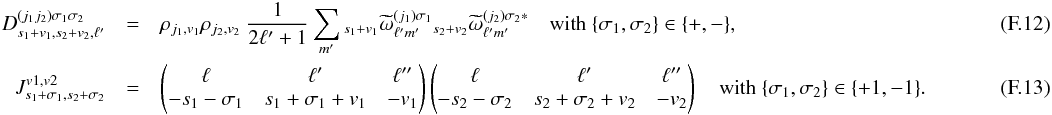 In the case of temperature, and assuming the beams to be circular, this simplifies to
 ![Mathematical equation: \appendix \setcounter{section}{6} \begin{eqnarray} \Delta \pC^{TT}_{\ell''} &=& \sum_{j_1 j_2 \ell} \ell(\ell+1) \frac{2\ell+1}{4\pi} C^{TT}_{\ell} \hatb^{(j_1)*}_{\ell 0} \, \hatb^{(j_2)}_{\ell 0} \nonumber \\ &&\ \times \sum_{\ell'} \frac{2\ell'+1}{4}\wjjj{\ell}{\ell'}{\ell''}{1}{-1}{0}^2 \left[ \left(D^{(j_1j_2)++}_{00, \ell'} + D^{(j_1j_2)--}_{00, \ell'}\right) - (-1)^{\ell+\ell'+\ell''}\left(D^{(j_1j_2)+-}_{00, \ell'} + D^{(j_1j_2)-+}_{00, \ell'}\right) \right] \end{eqnarray}](/articles/aa/full_html/2017/02/aa29626-16/aa29626-16-eq368.png) (F.14)in agreement with Planck Collaboration VII (2014), once one identifies
(F.14)in agreement with Planck Collaboration VII (2014), once one identifies  as the sum of the gradient and curl parts of the (spin 1) displacement field power spectrum and
  as their difference (see Sect. D).
It is instructive to further assume the relative location of the hit’s center of mass to be only weakly correlated between pixels, so that all its derived power spectra can be assumed to be white:  (i.e., with a variance
  in pixels of solid angle Ωpix = 4π/Npix). Equation (C.5) then ensures that the sub-pixel noise of Eq. (F.11) is also white, with constant polarized spectra
  (F.15)with
 ![Mathematical equation: \appendix \setcounter{section}{6} \begin{eqnarray} {\cal W}^{TT}_\ell &\! =\!&\frac{1}{4} \sum_{j_1 j_2 s}\left( \hatb^{(j_1)*}_{\ell s} \, \hatb^{(j_2)}_{\ell s} \left[ D^{(j_1j_2)++}_{ss} + D^{(j_1j_2)--}_{ss} \right] + \hatb^{(j_1)*}_{\ell s} \,\hatb^{(j_2)}_{\ell,s+2} D^{(j_1j_2)+-}_{s,s+2} + \hatb^{(j_1)*}_{\ell,s+2} \, \hatb^{(j_2)}_{\ell s} D^{(j_1j_2)-+}_{s+2,s}\right), \\ &\! \simeq\!&\frac{1}{4} \sum_{j_1 j_2} \hatb^{(j_1)*}_{\ell 0} \, \hatb^{(j_2)}_{\ell 0} \left[ D^{(j_1j_2)++}_{00} + D^{(j_1j_2)--}_{00} \right]; \\ {\cal W}^{EE}_{\ell} = {\cal W}^{BB}_{\ell} &\!=\!& \frac{1}{4} \sum_{j_1 j_2 s}\sum_{v=-2,2}\left( \hatb^{(j_1)*}_{\ell s} \, \hatb^{(j_2)}_{\ell s} \left[ D^{(j_1j_2)++}_{s+v,s+v} + D^{(j_1j_2)--}_{s+v,s+v} \right] + \hatb^{(j_1)*}_{\ell s} \,\hatb^{(j_2)}_{\ell,s+2} D^{(j_1j_2)+-}_{s+v,s+2+v} + \hatb^{(j_1)*}_{\ell,s+2} \, \hatb^{(j_2)}_{\ell s} D^{(j_1j_2)-+}_{s+2+v,s+v} \right), \\ &\!\simeq\!& \frac{1}{4} \sum_{j_1 j_2} \hatb^{(j_1)*}_{\ell 0} \, \hatb^{(j_2)}_{\ell 0} \left[ D^{(j_1j_2)++}_{22} + D^{(j_1j_2)--}_{22} + D^{(j_1j_2)++}_{-2-2} + D^{(j_1j_2)--}_{-2-2} \right]; \\ {\cal W}^{XY}_{\ell} &\!=\!& 0 \quad \text{when }X \ne Y~~~~~~~~~~~~~~~~~~~~~~~~~~~~~~~~~~~~~~~~~~~~~~~~~~~~~~~~~~~~~~~~~~~~~~~~~~~~~~~~~~~~~~~~~~~~~~~~~~~~~~~~~~~~~~~~~~~~~~~~~~~~~~~~~~~~~~~~~~~~~~~ \end{eqnarray}](/articles/aa/full_html/2017/02/aa29626-16/aa29626-16-eq375.png) where the approximate results are obtained for circular beams.
where the approximate results are obtained for circular beams.
Even for more realistic hypotheses on the hits locations, the sub-pixel contributions to the respective power spectra follow the hierarchy  (F.21)Let us consider now the other extra contribution to the power spectrum, involving the Laplacian of the sky signal and the quadratic norm of dr. Introducing
  where
where  is the second order moment of the hit location in pixel p. If we assume this and
  to be slowly varying functions of p, and consider ℓ ≫ s, the power spectra become
  (F.24)which describes to leading order, the smoothing effect of the integration of the signal on the pixel.
Appendix G: Co-polarized beam
For an arbitrarily shaped beam having the intensity harmonics coefficients  (G.1)and assumed to be perfectly co-polarized in direction γ, its polarized harmonics’ content will be
 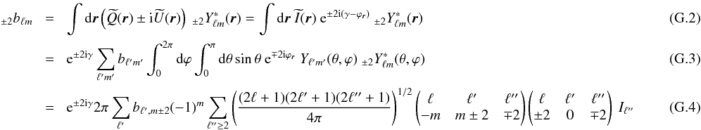 where we used Eq. (C.1) and introduced, for ℓ′′ ≥ 2
 Since Iℓ′′ peaks at ℓ′′ = 2, the 3J symbols will enforce ℓ′′ ≪ ℓ ≃ ℓ′ in Eq. (G.4). If the beam is narrow enough in real space, bℓ′,m will be almost constant over the allowed range ℓ−ℓ′′ ≤ ℓ′ ≤ ℓ + ℓ′′, and we use the approximate orthogonality relation of Eq. (C.9) to write
  (G.8)Finally, we note that in Eq. (G.4), the sum
  to obtain
  (G.12)which is valid for any (narrow) co-polarized beam.
All Figures
|
Fig. 1 Orientation of polarization measurements in Planck. The two left panels show, for an actual Planck detector, the maps of ⟨cos2α⟩ and ⟨sin2α⟩ respectively, where α is the direction of the polarizer with respect to the local Galactic meridian, which contributes to the spin 2 term |
| In the text | |
|
Fig. 2 Same as Fig. 1 for an hypothetical detector of a LiteBIRD-like mission, except for the right panel plot which has a different y-range. |
| In the text | |
|
Fig. 3 Effective beam window matrix |
| In the text | |
|
Fig. 4 Computer simulated beam maps ( |
| In the text | |
|
Fig. 5 Comparison to simulations for 100ds1x217ds1 (lhs panels) and 143ds1x217ds1 (rhs panels) cross power spectra, for computer simulated beams. In each panel is shown the discrepancy between the actual ℓ(ℓ + 1)Cℓ/ 2π and the one in input, smoothed on Δℓ = 31. Results obtained on simulations with either the full beam model (green curves) or the co-polarized beam model (blue dashes) are to be compared to QuickPol analytical results (red long dashes). In panels where it does not vanish, a small fraction of the input power spectrum is also shown as black dots for comparison. |
| In the text | |
Current usage metrics show cumulative count of Article Views (full-text article views including HTML views, PDF and ePub downloads, according to the available data) and Abstracts Views on Vision4Press platform.
Data correspond to usage on the plateform after 2015. The current usage metrics is available 48-96 hours after online publication and is updated daily on week days.
Initial download of the metrics may take a while.