| Issue |
A&A
Volume 598, February 2017
|
|
|---|---|---|
| Article Number | A51 | |
| Number of page(s) | 11 | |
| Section | Extragalactic astronomy | |
| DOI | https://doi.org/10.1051/0004-6361/201629380 | |
| Published online | 01 February 2017 | |
Novel calibrations of virial black hole mass estimators in active galaxies based on X-ray luminosity and optical/near-infrared emission lines
1 Dipartimento di Matematica e Fisica, Università Roma Tre, via della Vasca Navale 84, 00146 Roma, Italy
e-mail: This email address is being protected from spambots. You need JavaScript enabled to view it.
2 SRON, Netherlands Institute for Space Research, Sorbonnelaan 2, 3584 CA, Utrecht, The Netherlands
3 Department of Astrophysics/IMAPP, Radboud University, PO Box9010, 6500 GL Nijmegen, The Netherlands
Received: 22 July 2016
Accepted: 3 October 2016
Abstract
Context. It is currently only possible to accurately weigh, through reverberation mapping (RM), the masses of super massive black holes (BHs) in active galactic nuclei (AGN) for a small group of local and bright broad line AGN. Statistical demographic studies can be carried out considering the empirical scaling relation between the size of the broad line region (BLR) and the AGN optical continuum luminosity. There are still biases, however, against low-luminosity or reddened AGN, in which the rest-frame optical radiation can be severely absorbed or diluted by the host galaxy and the BLR emission lines can be hard to detect.
Aims. Our purpose is to widen the applicability of virial-based single-epoch (SE) relations to measure reliably the BH masses for low-luminosity or intermediate and type 2 AGN, which the current methodology misses. We achieve this goal by calibrating virial relations based on unbiased quantities: the hard X-ray luminosities in the 2–10 keV and 14–195 keV bands that are less sensitive to galaxy contamination, and the full width at half maximum (FWHM) of the most important rest-frame near-infrared (NIR) and optical BLR emission lines.
Methods. We built a sample of RM AGN with both X-ray luminosity, broad optical and NIR FWHM measurements available to calibrate new virial BH mass estimators.
Results. We found that the FWHM of the Hα, Hβ, and NIR lines (i.e. Paα, Paβ, and He iλ10830) all correlate with each other with negligible or small offsets. This result allowed us to derive virial BH mass estimators based on either the 2–10 keV or 14–195 keV luminosity. We also took into account the recent determination of the different virial coefficients, f, for pseudo- and classical bulges. By splitting the sample according to the bulge type and adopting separate f factors, we found that our virial relations predict BH masses of AGN hosted in pseudo-bulges ~0.5 dex smaller than in classical bulges. Assuming the same average f factor for both populations, a difference of ~0.2 dex is still found.
Key words: galaxies: active / galaxies: nuclei / galaxies: bulges / quasars: emission lines / quasars: supermassive black holes / X-rays: galaxies
© ESO, 2017
1. Introduction
Supermassive black holes (SMBHs, with black hole masses MBH = 105−109M⊙), are observed to be common, hosted in the central spheroid in the majority of local galaxies. This discovery, combined with the observation of striking empirical relations between black hole (BH) mass and host galaxy properties, opened an exciting era in extragalactic astronomy in the last two decades. In particular the realization that BH mass correlates strongly with the stellar luminosity, mass, and velocity dispersion of the bulge (Dressler 1989; Kormendy & Richstone 1995; Magorrian et al. 1998; Ferrarese & Merritt 2000; Gebhardt et al. 2000; Marconi & Hunt 2003; Sani et al. 2011; Graham 2016, for a review) suggests that SMBHs may play a crucial role in regulating many aspects of galaxy formation and evolution, for example, through AGN feedback (Silk & Rees 1998; Fabian 1999, 2012; Di Matteo et al. 2005; Croton et al. 2006; Sijacki et al. 2007; Ostriker et al. 2010; King 2014).
One of the most reliable and direct ways to measure the mass of a SMBH residing in the nucleus of an active galaxy (i.e. an active galactic nucleus; AGN) is reverberation mapping (RM; Blandford & McKee 1982; Peterson 1993). The RM technique takes advantage of AGN flux variability to constrain black hole masses through time-resolved observations. With this method, the distance R = cτ of the broad line region (BLR) is estimated by measuring the time lag τ of the response of a permitted broad emission line to the variation of the photoionizing primary continuum emission. Under the hypothesis of a virialized BLR, whose dynamics are gravitationally dominated by the central SMBH, MBH is simply related to the velocity of the emitting gas clouds, Δv, and to the size R of the BLR, i.e. MBH = Δv2RG-1 , where G is the gravitational constant. Usually the width ΔW of a doppler-broadened emission line (i.e. the full width at half maximum; FWHM, or the line dispersion, σline) is used as a proxy of the real gas velocity Δv, after introducing a virial factor f that takes into account our ignorance of the structure, geometry, and kinematics of the BLR (Ho 1999; Wandel et al. 1999; Kaspi et al. 2000),  (1)Operatively, the RM BH mass is equal to f × Mvir, where the virial mass Mvir is ΔW2RG-1. In the last decade, the f factor has been studied by several authors, finding values in the range 2.8–5.5 if the line dispersion σline is used (see e.g. Onken et al. 2004; Woo et al. 2010; Graham et al. 2011; Park et al. 2012; Grier et al. 2013). This quantity is statistically determined by normalizing the RM AGN to the relation between BH mass and bulge stellar velocity dispersion (MBH−σ⋆ relation; see Ferrarese 2002; Tremaine et al. 2002; Hu 2008; Gültekin et al. 2009; Graham & Scott 2013; McConnell & Ma 2013; Kormendy & Ho 2013; Savorgnan & Graham 2015; Sabra et al. 2015) observed in local inactive galaxies with direct BH mass measurements. However, recently Shankar et al. (2016) claimed that the previously computed f factors could have been artificially increased by a factor of at least ~3 because of a presence of a selection bias in the calibrating samples in favour of more massive BHs. Kormendy & Ho (2013) significantly updated the MBH−σ⋆ relation for inactive galaxies, highlighting a large and systematic difference between the relations for pseudo- and classical bulges and/or ellipticals. The classification of galaxies into classical and pseudo-bulges is, however, a difficult task, which depends on a number of selection criteria. These criteria should not be used individually; for example, the Sersic index (Sersic 1968) n< 2 condition alone does not classify a source as a pseudo-bulge (e.g. see Kormendy & Ho 2013; Kormendy 2016). Some authors have also discussed how it could be neither appropriate nor possible to reliably separate bulges into one class or another (Graham 2014), and that in some galaxies there is evidence of a coexistence of classical bulges and pseudo-bulges (Erwin et al. 2015; Dullo et al. 2016).
The results on the MBH−σ⋆ found by Kormendy & Ho (2013) prompted Ho & Kim (2014) to calibrate the f factor separately for the two bulge populations obtaining fCB = 6.3 ± 1.5 for elliptical and/or classical and fPB = 3.2 ± 0.7 for pseudo-bulges when the Hβσline (not the FWHM) is used to compute the virial mass, otherwise the virial coefficient f has to be scaled depending on the FWHM/σline ratio (see e.g. Onken et al. 2004; Collin et al. 2006, for details). For a similar approach, see also Graham et al. (2011) who derived different MBH−σ⋆ relations and f factors for barred and non-barred galaxies.
However, RM campaigns are time consuming and are accessible only for a handful of nearby (i.e. z ≲ 0.1) AGN. The finding of a tight relation between the distance of the BLR clouds R and the AGN continuum luminosity L (R ∝ L0.5; Bentz et al. 2006, 2013) has allowed the calibration of new single-epoch (SE) relations that can be used on larger samples of AGN, such as ![Mathematical equation: \begin{equation} \label{eq:cal} \log \left(\frac{M_{ \mathrm{BH}} }{M_\odot}\right) = a + b \log \left[ \left(\frac{L}{10^{42}~ \mathrm{erg \, s^{-1}} }\right)^{0.5} \left(\frac{{\it FWHM}}{10^4 ~\mathrm{km\, s^{-1} }}\right)^2 \right] ; \end{equation}](/articles/aa/full_html/2017/02/aa29380-16/aa29380-16-eq27.png) (2)where the term log (L0.5 × FWHM2) is generally known as virial product (VP). These SE relations have a typical spread of ~0.5 dex (e.g. McLure & Jarvis 2002; Vestergaard & Peterson 2006). These relations are calibrated with either the broad emission line or the continuum luminosity (e.g. in the ultraviolet and optical, mostly at 5100 Å, L5100; see the review by Shen 2013, and references therein) and the FWHM (or the σline) of optical emission lines, such as Hβ, Mg ii λ2798, and C iv λ1549, even though the latter is still a matter of debate (e.g. Baskin & Laor 2005; Shen & Liu 2012; Denney 2012; Runnoe et al. 2013). As the calibrating RM masses are computed by measuring the BLR line width and its average distance R = cτ, the fit of Eq. (2) corresponds, strictly speaking, to the fit of the τ versus L relation (e.g. Bentz et al. 2006).
(2)where the term log (L0.5 × FWHM2) is generally known as virial product (VP). These SE relations have a typical spread of ~0.5 dex (e.g. McLure & Jarvis 2002; Vestergaard & Peterson 2006). These relations are calibrated with either the broad emission line or the continuum luminosity (e.g. in the ultraviolet and optical, mostly at 5100 Å, L5100; see the review by Shen 2013, and references therein) and the FWHM (or the σline) of optical emission lines, such as Hβ, Mg ii λ2798, and C iv λ1549, even though the latter is still a matter of debate (e.g. Baskin & Laor 2005; Shen & Liu 2012; Denney 2012; Runnoe et al. 2013). As the calibrating RM masses are computed by measuring the BLR line width and its average distance R = cτ, the fit of Eq. (2) corresponds, strictly speaking, to the fit of the τ versus L relation (e.g. Bentz et al. 2006).
But these empirical scaling relations have some problems:
-
Broad Fe ii emission in type 1AGN (AGN1) can add ambiguity in the determination of theoptical continuum luminosity at5100 Å.
-
In low-luminosity AGN, host galaxy starlight dilution can severely affect the AGN ultraviolet and optical continuum emission. Therefore in such sources it becomes very challenging, if not impossible, to isolate the AGN contribution unambiguously.
-
The Hβ transition is at least a factor of three weaker than Hα and hence, from considerations of signal-to-noise ratio (S/N) alone, Hα, if available, is superior to Hβ. In practice, in some cases Hα may be the only line with a detectable broad component in the optical (such objects are known as Seyfert 1.9 galaxies; Osterbrock 1981).
-
The optical SE scaling relations are completely biased against type 2 AGN (AGN2), which lack broad emission lines in the rest-frame optical spectra. However, several studies have shown that most AGN2 exhibit faint components of broad lines if observed with high (≳20) S/N in the rest-frame near-infrared (NIR), where the dust absorption is less severe than in the optical (Veilleux et al. 1997; Riffel et al. 2006; Cai et al. 2010; Onori et al. 2017). Moreover, some studies have shown that NIR lines (i.e. Paα and Paβ) can be reliably used to estimate the BH masses in AGN1 (Kim et al. 2010, 2015; Landt et al. 2013) and for intermediate or type 2 AGN (La Franca et al. 2015, 2016).
In an effort to widen the applicability of such relations to classes of AGN that would otherwise be inaccessible using the conventional methodology (e.g. galaxy-dominated low-luminosity sources, type 1.9 Seyfert and type 2 AGN), La Franca et al. (2015) fitted new virial BH mass estimators based on intrinsic (i.e. absorption corrected) hard X-ray luminosity in the 14–195 keV band; this emission is thought to be produced by the hot corona via Compton scattering of the ultraviolet and optical photons coming from the accretion disk (Haardt & Maraschi 1991; Haardt et al. 1994, 1997). Actually the X-ray luminosity LX is known to be empirically related to the dimension of the BLR, as it is observed for the optical continuum luminosity of the AGN accretion disk (e.g. Maiolino et al. 2007; Greene et al. 2010). Thanks to these R−LX empirical scaling relations, Bongiorno et al. (2014) have also derived virial relations based on the Hα width and on the hard, 2–10 keV, X-ray luminosity, which is less affected by galaxy obscuration (excluding severely absorbed, Compton thick AGN, NH> 1024 cm-2). Indeed, in the 14–195 keV band up to NH< 1024 cm-2 the absorption is negligible, while in the 2–10 keV band the intrinsic X-ray luminosity can be recovered after measuring the NH column density via X-ray spectral fitting.
Recently Ho & Kim (2015) showed that the BH masses of RM AGN correlates tightly and linearly with the optical VP (i.e. FHWM(Hβ) ) with different logarithmic zero points for elliptical (and/or classical) and pseudo-bulges. These authors used the updated database of RM AGN with bulge classification from Ho & Kim (2014) and adopted the virial factors separately for classical (fCB = 6.3) and pseudo-bulges (fPB = 3.2).
Prompted by these results, in this paper we present an update of the calibrations of the virial relations based on the hard 14–195 keV X-ray luminosity published in La Franca et al. (2015). We extend these calibrations to the 2–10 keV X-ray luminosity and to the most intense optical and NIR emission lines, i.e. Hβλ4862.7 Å, Hαλ6564.6 Å, He iλ10830.0 Å, Paβλ12821.6 Å, and Paαλ18756.1 Å. In order to minimize the statistical uncertainties in the estimate of the parameters a and b of the virial relation (Eq. (2)), we verified that reliable statistical correlations exist among the hard X-ray luminosities, L2−10 keV and L14−195 keV, and among the optical and NIR emission lines (as already found by other studies; Greene & Ho 2005; Landt et al. 2008; Mejía-Restrepo et al. 2016). These correlations allowed us first, to compute, using the total dataset, the average FWHM and LX for each object and then derive more statistically robust virial relations; second, to compute our BH mass estimator using any combination of LX and optical or NIR emission line width.
We proceed as follows: Sect. 2 presents the RM AGN dataset; in Sect. 3 we test whether the optical (i.e. Hα and Hβ) and NIR (i.e. Paα, Paβ , and He iλ10830 Å; hereafter He i) emission lines probe similar region in the BLR; in Sect. 4 we present new calibrations of the virial relations based on the average hard X-ray luminosity and the average optical and NIR emission lines width, taking (or not) into account the bulge classification; and finally Sect. 5 addresses the discussion of our findings and the conclusions. Throughout the paper we assume a flat ΛCDM cosmology with cosmological parameters ΩΛ = 0.7, ΩM = 0.3 and H0 = 70 km s-1 Mpc-1. Unless otherwise stated, all the quoted uncertainties are at 68% (1σ) confidence level.
Properties of the RM AGN with both bulge classification and hard X-ray luminosity.
Properties of the additional AGN1 database used in the emission line relation analysis.
2. Data
As we are interested in expanding the applicability of SE relations, we decided to use emission lines that can be more easily measured also in low-luminosity or obscured sources, such as the Hα or the Paα, Paβ, and He i. Moreover, we also want to demonstrate that such lines can give as reliable estimates as those derived using the Hβ (see e.g. Greene & Ho 2005; Landt et al. 2008; Kim et al. 2010; Mejía-Restrepo et al. 2016). For this reason, we built our sample starting from the database of Ho & Kim (2014), which lists 43 RM AGN (i.e. ~90% of all the RM black hole masses available in the literature), which all have bulge-type classifications based on the criteria of Kormendy & Ho (2013, supplemental material). In particular, Ho & Kim (2014) used the most common condition to classify those galaxies having Sersic index (Sersic 1968) n< 2 as pseudo-bulges. However when the nucleus is too bright this condition is not totally reliable because of the difficulty of carefully measuring the bulge properties. In this case Ho & Kim (2014) adopted the condition that the bulge-to-total light fraction should be ≲0.2 (e.g. Fisher & Drory 2008; Gadotti 2009, but see Graham & Worley 2008, for a discussion on the uncertainties of this selection criterion). In some cases, additional clues came from the detection of circumnuclear rings and other signatures of ongoing central star formation.
It should be noted that an offset (~0.3 dex) is observed in the MBH−σ⋆ diagram both when the galaxies are divided into barred and unbarred (e.g. Graham 2008; Graham et al. 2011; Graham & Scott 2013) and into classical and pseudo-bulges (Hu 2008). However, the issue on the bulge-type classification and on which host properties better discriminate the MBH−σ⋆ relation is beyond the scope of this work, and in the following we adopt the bulge-type classification as described in Ho & Kim (2014).
Among this sample, we selected those AGN with available hard X-ray luminosity and at least one emission line width among Hβ, Hα, Paα, Paβ, and He i. The data of 3C 390.3 were excluded since it clearly shows a double-peaked Hα profile (Burbidge & Burbidge 1971; Dietrich et al. 2012), which is a feature that could be a sign of non-virial motions (in particular of accretion disk emission, e.g. Eracleous & Halpern 1994, 2003; Gezari et al. 2007). Therefore our dataset is composed as follows:
-
1.
Hβ sample. The largest sample considered in this work includes 39 RM AGN with Hβ FWHM coming either from a mean or a single spectrum. By requiring that these AGN have an X-ray luminosity measured either in the 2–10 keV or 14–195 keV band reduces the sample to 35 objects.
-
2.
Hα sample. There are 33 AGN with Hα FWHM, but we excluded the source Mrk 202 as the Hα FWHM is deemed to be unreliable (Bentz et al. 2010). Therefore, 32 AGN have Hα FWHM. Among this sample, Mrk 877 and SBS 1116+583A do not have an LX measurement available. Thus the final sample, with available both Hα FWHM and X-ray luminosity, includes 30 galaxies.
-
3.
NIR sample. The FWHM of the NIR emission lines were taken from Landt et al. (2008, 2013, i.e. 19 Paα, 20 Paβ, and 16 He i. We added the measurements of NGC 3783 that we observed simultaneously in the ultraviolet, optical, and NIR with Xshooter (Onori et al. 2017). Therefore the total NIR sample, with available X-ray luminosity, amounts to19 Paα, 21 Paβ, and 17 He i.
The details of each RM AGN are reported in Table 1. The intrinsic hard X-ray luminosities have been taken either from the SWIFT/BAT 70 month catalogue (14–195 keV, L14−195 keV; Baumgartner et al. 2013) or from the CAIXA catalogue (2–10 keV, L2−10 keV; Bianchi et al. 2009). PG 1411+442 has public 2–10 keV luminosity from Piconcelli et al. (2005), while Mrk 1310 and NGC 4748 have public XMM observations; therefore we derived their 2–10 keV luminosity via X-ray spectral fitting. Both X-ray catalogues list the 90% confidence level uncertainties on the LX and/or on the hard X-ray fluxes, which were converted into the 1σ confidence level. For PG 1411+442, as the uncertainty on the L2−10 keV has not been published (Piconcelli et al. 2005), a 6% error (equivalent to 10% at the 90% confidence level) has been assumed. All the FWHMs listed in Table 1 have been corrected for instrumental resolution broadening. When possible, we always preferred to use coeval (i.e. within few months) FWHM measurements of the NIR and optical lines. This choice is dictated by the aim of verifying whether the optical and NIR emission lines are originated at a similar distance in the BLR. The virial masses have been taken mainly from the compilations of Grier et al. (2013) and Ho & Kim (2014) and were computed from the σline(Hβ), measured from the root mean square (rms) spectra, taken during RM campaigns, and the updated Hβ time lags (see Zu et al. 2011; Grier et al. 2013). For 3C 273 and Mrk 335, the logarithmic mean of the measurements available (Ho & Kim 2014) were used.
To the data presented in Table 1, we also added six AGN1 from Landt et al. (2008, 2013, see Table 2 that have neither RM MBH nor bulge classifications, but have simultaneous measurements of optical and/or NIR lines. These AGN1 are the following: H 1821+643, H 1934-063, H 2106-099, HE 1228+013, IRAS 1750+508, and PDS 456. Table 2 also lists the optical data of Mrk 877 and SBS 1116+583A. These additional eight sources that do not appear in Table 1 are used only in the next section in which emission line relations are investigated.
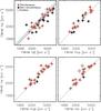 |
Fig. 1 Linear relations between the FWHM of Hα and the FWHM of Hβ, Paα, Paβ, or He i, from left to right and top to bottom. Red filled circles denote simultaneous observations of the two lines, while black filled circles describe non-simultaneous line measurements. Grey open squares indicate the measurements that are classified as outliers (see text for more details) and are not considered in the fits. The black dotted line shows the 1:1 relation in all panels. In the top left panel, the best-fit relation computed on the coeval sample is shown as a red solid line. The relations from Greene & Ho (2005, dashed cyan) and Mejía-Restrepo et al. (2016, dashed blue) are also reported. |
3. Emission line relations
As suggested by several works (e.g. Greene & Ho 2005; Shen & Liu 2012; Mejía-Restrepo et al. 2016), the strongest Balmer lines, Hα and Hβ, seem to come from the same area of the BLR. If we confirm that a linear correlation between H i and He i optical and NIR lines (i.e. Paα, Paβ, and He i) exists, this result has two consequences: it will indicate that these lines come from the same region of the BLR, and that the widely assumed virialization of Hβ also implies the virialization of the Hα and NIR lines.
Figure 1 shows the results of our analysis, by comparing the FWHM of Hα with the FWHMs of the Hβ, Paα, Paβ, and He i lines. In all panels the coeval FWHMs are shown with red filled circles while those not coeval are indicated with black filled circles. Although in some cases the uncertainties are reported in the literature, following the studies of Grupe et al. (2004), Vestergaard & Peterson (2006), Landt et al. (2008), and Denney et al. (2009), we assumed a common uncertainty of 10% on the FWHM measurements.
The top left panel of Fig. 1 shows the relation between the two Balmer emission lines. We find a good agreement between the FWHMs of Hα and Hβ. Using the sub-sample of 23 sources with simultaneous measurements, the Pearson correlation coefficient results to be r ≃ 0.92, with a probability of being drawn from an uncorrelated parent population as low as ~6 × 10⁻¹⁰. The least-squares problem was solved using the symmetrical regression routine FITEXY (Press et al. 2007), which can incorporate errors on both variables and allows us to account for intrinsic scatter. We fitted a log-linear relation to the simultaneous sample and found  (3)The above relation means that Hβ is on average 0.075 dex broader than Hα, with a scatter of ~0.08 dex. This relation has a reduced
  . We performed the F-test to verify the significance of this non-zero offset with respect to a 1:1 relation, getting a probability value of ~2 × 10⁻⁴ that the improvement of the fit was obtained by chance. Throughout this work in the F-test we use a threshold of 0.012, corresponding to a 2.5σ Gaussian deviation to rule out the introduction of an additional fitting parameter. Therefore in this case the relation with a non-zero offset resulted to be highly significant. We also tested whether this offset changes according to the bulge classification, when available. No significant difference was found, as the offset was 0.076 ± 0.020 for the pseudo-bulges and 0.074 ± 0.020 for the elliptical or classical bulges.
Equation (3) is shown as a red solid line in the top left panel of Fig. 1. Our result is in fair agreement (i.e. within 2σ) with other independent estimates, which are shown with cyan (Greene & Ho 2005) and blue (Mejía-Restrepo et al. 2016) dashed lines. If instead we consider the total sample of 34 AGN having both Hα and Hβ measured (i.e. including also non-coeval FWHMs), we get an average offset of 0.091 ± 0.010 with a larger scatter (~0.1 dex). Also in this case, the offset does not show a statistically significant dependence on the bulge classification, as the offset was 0.102 ± 0.014 for elliptical and/or classical bulges and 0.080 ± 0.019 for pseudo-bulges. In all the aforementioned fits, we excluded three outliers1 even though the FWHMs were measured simultaneously. These excluded galaxies are Mrk 1310, Mrk 590, and NGC 5548. The first galaxy was excluded because the Hα measurement is highly uncertain ( km s-1; Bentz et al. 2010), and the latter two have extremely broader Hβ than Hα, Paα, Paβ, and He i. This fact is because of the presence of a prominent “red shelf” in the Hβ of these two sources (Landt et al. 2008). This red shelf is also most likely responsible for the average trend observed between Hβ and Hα, i.e. that Hβ is on average broader than Hα (Eq. (3)). Indeed it is well known (e.g. De Robertis 1985; Marziani et al. 1996, 2013) that the Hβ broad component is in part blended with weak Fe ii multiplets, He iiλ4686 and He iλ4922, 5016 (Véron et al. 2002; Kollatschny et al. 2001). The simultaneous sample gives a relation with lower scatter than the total sample. Indeed, the non-simultaneous measurements introduce additional noise due to the well-known AGN variability phenomenon. Therefore in the following sections we use the average offset between the FWHM of Hα and Hβ computed using the coeval sample (i.e. Eq. (3)), which also better agrees with the relations already published by Greene & Ho (2005) and Mejía-Restrepo et al. (2016).
Results of the fits of the virial relations.
The other three panels of Fig. 1 show the relations between the Hα and the NIR emission lines Paα (19 objects) , Paβ (22), and He i (19). When compared to Hα, the samples have Pearson correlation coefficient r of 0.92, 0.94, and 0.95, with probabilities of being drawn from an uncorrelated parent population as low as ~2 × 10-8,9 × 10-11, and 5 × 10⁻¹⁰ for the Paα, Paβ, and He i, respectively. No significant difference is seen between the emission line widths of the Hα and NIR lines. This is not surprising as Landt et al. (2008) already noted that there was a good agreement between the FWHM of the Paβ and the two strongest Balmer lines, although an average trend of Hβ being larger than Paβ was suggested (a quantitative analysis was not carried out). We fitted log-linear relations to the data and always found that the 1:1 relation is the best representation of the sample. We found a reduced  of 1.54, 1.12, and 1.14 for Paα, Paβ, and He i, respectively. The F-test was carried out to verify quantitatively whether the equality relations are preferred with respect to relations with a non-zero offset or those including a free slope. The improvements obtained with the free-slope relations were not highly significant, and therefore the more physically motivated 1:1 relations were preferred. These best-fitting relations are shown as black dotted lines in the remaining three panels of Fig. 1. The relation between Hα and the Paβ emission line has been fitted using the whole sample, while for the Paα and He i correlations we excluded the sources NGC 7469 (for the Paα), Mrk 79, and NGC 4151 (for He i; shown as grey open squares in the bottom right panel of Fig. 1). Although these three sources have simultaneous optical and NIR observations (Landt et al. 2008), all show a significantly narrower width of the Paα or He i emission lines than all the other available optical and NIR emission lines.
4. Virial mass calibrations
In the previous section we showed that the Hα FWHM is equivalent to the widths of the NIR emission lines, Paα, Paβ, and He i, while it is on average 0.075 dex narrower than Hβ. In order to minimize the uncertainties on the estimate of the zero point and slope that appear in Eq. (2) we used the whole dataset listed in Table 1. This is possible because, besides the linear correlations between the optical and NIR FWHMs, the intrinsic hard X-ray luminosities L2−10 keV and L14−195 keV are also correlated. Indeed, as expected in AGN, we found a relation between the two hard X-ray luminosities  (4)which corresponds to an average X-ray photon index ⟨ Γ ⟩ ≃ 1.67 (fν ∝ ν− (Γ−1)). We can therefore calculate, for each object of our sample, a sort of average VP, which has been computed using the average FWHM of the emission lines (the Hβ has been converted into Hα by using Eq. (3)) and the average X-ray luminosity (converted into 2–10 keV band using Eq. (4)). When computing the average FWHM, the values that were considered outliers in the previous section were again excluded. However we note that each RM AGN has at least one valid FWHM measurement, therefore none of the AGN were excluded. This final RM AGN sample is the largest with available bulge classification (Ho & Kim 2015) and hard LX and counts a total of 37 sources, 23 of which are elliptical and/or classical and 14 are pseudo-bulges. This sample is made of all sources with hard X-ray luminosity measurements among those of Ho & Kim (2014), whose sample of bulge-classified RM AGN includes ~90% of all the RM black hole masses available in the literature.
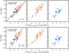 |
Fig. 2 Virial relations between the BH mass MBH = f × Mvir and the average VP given by the mean FWHM (once the Hβ has been converted into Hα) and the mean L2−10 keV (using Eq. (4) to convert L14−195 keV). In the top panels the black hole masses have been calculated assuming ⟨ f ⟩ = 4.31 (Grier et al. 2013), while in the bottom panels two different f factors, fCB = 6.3 for classical bulges and fPB = 3.2 for pseudo-bulges (Ho & Kim 2014), have been adopted to determine MBH. All the VPs are normalized as specified in Eq. (2) (see Tables 3, 4 for the resulting best-fit parameters). In the left panels the total calibrating sample is shown, while in the middle and right panels the sub-samples of classical (red filled squares) and pseudo-bulges (blue open squares) are shown separately. The lines show the best-fitting virial relations derived for each sample. |
We want to calibrate the linear virial relation given in Eq. (2), where MBH is the RM black hole mass, which is equal to f × Mvir, a is the zero point, and b is the slope of the average VP. We fitted Eq. (2) for the whole sample of RM AGN assuming one of the most updated virial factors, ⟨ f ⟩ = 4.31 (Grier et al. 2013), which does not depend on the bulge morphology. The data have a correlation coefficient r = 0.838, corresponding to a probability as low as ~9 × 10-11 that the data are randomly extracted from an uncorrelated parent population. As previously carried out in Sect. 3, we performed a symmetrical regression fit using FITEXY (Press et al. 2007). We first fixed the slope b to unity finding the zero point a = 8.032 ± 0.014. The resulting observed spread ϵobs is 0.40 dex, while the intrinsic spread ϵintr (i.e. once the contribution from the data uncertainties has been subtracted in quadrature) is 0.38 dex. We also performed a linear regression, allowing the slope b to vary. The F-test was carried out to verify quantitatively whether our initial assumption of fixed slope had to be preferred to a relation with a free slope. The F-test gave a probability of ~0.07, which is not significantly small enough to demonstrate that the improvement using a free slope is not obtained by chance. Therefore, we preferred the use of the more physically motivated relation (having slope b = 1), which depends only linearly on the VP. The resulting best-fitting parameters are reported in Table 3, while the virial relation is shown in the top left panel of Fig. 2 (black solid line).
We then splitted the sample into elliptical and/or classical (23) and pseudo-bulges (14), adopting the same virial factor ⟨ f ⟩ = 4.31. The two samples have a correlation coefficient r > 0.7 with probabilities lower than ~10-3 that the data have been extracted randomly from an uncorrelated parent population (see Table 3). Again we first fixed the slope b to unity, obtaining the zero points a = 8.083 ± 0.016 and a = 7.911 ± 0.026 for classical and pseudo-bulges, respectively. We also performed a linear regression allowing a free slope. The F-test was carried out and gave probabilities greater than 0.05 for both the classical and the pseudo-bulge samples. Therefore the more physically motivated relations that depend linearly on the VP were preferred, as previously found for the whole sample. Top middle and top right panels of Fig. 2 show the resulting best-fit virial relations for classical (in red) and pseudo-bulges (in blue). It should be noted that the average difference between the zero points a of the two bulge-type populations is ~0.2 dex.
Obviously, the same fitting results, using these two sub-samples separately, are obtained if the recently determined different f factors of 6.3 and 3.2 for classical and pseudo-bulges (Ho & Kim 2014) are adopted. However, as expected, the difference between the zero points of the two populations becomes larger (~0.5 dex) as the zero points are a = 8.248 ± 0.016 and a = 7.782 ± 0.026 for the classical and pseudo-bulges, respectively.
Finally we performed a calibration of Eq. (2) for the whole sample, adopting the two virial factors fCB = 6.3 and fPB = 3.2 according to the bulge morphological classification. The correlation coefficient of the data is r = 0.831 with a probability as low as ~10-10 to have been drawn randomly from an uncorrelated parent population. As previously described, we first fixed the slope b to unity and then fitted a free slope. The F-test gave a probability lower than 0.01, therefore the solution with slope b = 1.376 ± 0.033 was in this case considered statistically significant (see Table 3). The observed and intrinsic spreads were ~0.5 dex (see Table 3). We note that a slope different than unity imply that the LX−R relation (R ∝ Lα) has a power α ≠ 0.5, in contrast to what was found by Greene et al. (2010). The bottom panels of Fig. 2 show the virial relations that we obtained for the whole sample (left panel, black dot-dashed line) and separately for classical (middle panel, red dashed line) and pseudo-bulges (right panel, blue dotted line), once the two different virial factors f were adopted according to the bulge morphology.
It is possible to convert our virial calibrations − which were estimated using the mean line widths, once converted into the Hα FWHM, and the mean X-ray luminosity, once converted into the L2−10 keV− into other equivalent relations based on the Hβ, Paα, Paβ, and He i FWHM and the L14−195 keV using the correlations shown in Eqs. (3) and (4). To facilitate the use of our virial BH mass estimators, we list in Table 4 how the virial zero point a changes according to the couple of variables that one wishes to use. Moreover, as shown in the virial relation in the top part of Table 4, it is possible to convert the resulting BH masses for different assumed virial f factors adding the term log (f/f0), where f0 is the virial factor that was assumed when each sample was fitted. The values of f0 are also reported in Table 4 for clarity. In the last case, where a solution was found for the total sample using separate f factors for classical and pseudo-bulges, the log (f/f0) correction cannot be used. However, this last virial relation is useful in those cases where the bulge morphological type is unknown and one wishes to use a solution that takes into account the two virial factors for classical and pseudo-bulges as measured by Ho & Kim (2014). Otherwise, the virial BH mass estimator calculated fitting the whole dataset assuming a single ⟨ f ⟩ = 4.31 can be used (and if necessary converted adopting a different average f factor).
Final virial BH mass estimators.
We compared the virial relation derived by La Franca et al. (2015) using the Paβ and L14−195 keV with our two new virial relations. These relations depend on the VP given by the Hα FWHM and L14−195 keV, obtained using the total sample, and assuming either an average virial factor, ⟨ f ⟩ = 4.31 (as used in La Franca et al. 2015), or the two different f, separately for classical and pseudo-bulges. Our two new virial relations give BH masses similar to the relation of La Franca et al. (2015) at MBH ~ 107.5M⊙, while they predict 0.3 (0.8) dex higher BH masses at MBH ~ 108.5M⊙ and 0.2 (0.7) dex lower masses at MBH ~ 106.5M⊙, assuming the average ⟨ f ⟩ = 4.31 (the two f factors fCB = 6.3, fPB = 3.2). These differences are due to the samples used: our dataset includes 15 AGN with MBH ≳ 108M⊙, while in the La Franca et al. (2015) sample there are only three, and at MBH ≲ 107M⊙ our dataset is a factor two larger.
The same comparison was carried out using the VP given by the Hα FWHM and L2−10 keV with the analogous relation in Bongiorno et al. (2014). All the relations predict similar masses in the MBH ~ 107.5M⊙ range, while our new calibrations give 0.1 (0.2) dex smaller (higher) masses at MBH ~ 108.5M⊙ and 0.2 (0.1) dex bigger (lower) BH masses at MBH ~ 106.5M⊙, assuming the average ⟨ f ⟩ = 4.31 (the two f factors fCB = 6.3, fPB = 3.2).
Finally our analysis shows some similarities with the results of Ho & Kim (2015), who recently calibrated SE optical virial relations based on the Hβ FWHM and L1500, using the total calibrating sample of RM AGN, and separately according to the bulge morphology into classical and pseudo-bulges. They found that in all cases the MBH depends on the optical VP with slope b = 1 and with different zero points a for classical and pseudo-bulges. This difference implies that BH hosted in pseudo-bulges are predicted to be 0.41 dex less massive than in classical bulges. When we adopt the same f factors used by Ho & Kim (2015), we similarly find that the zero point a of classical bulges is ~0.5 dex greater than for pseudo-bulges. However we do not confirm their result obtained using the total sample, as we find that the best-fitting parameter b of our VP should be different than one. At variance when the same average ⟨ f ⟩ = 4.31 is adopted, both in the total and in the sub-samples of classical and pseudo-bulges, we find slope b = 1 relations, while the zero points of classical and pseudo-bulges still show an offset of ~0.2 dex.
5. Discussion and conclusions
This work was prompted by the results of Ho & Kim (2015) who have calibrated optical different virial relations according to the bulge morphological classification into classical and/or elliptical and pseudo-bulges (Ho & Kim 2014). Following La Franca et al. (2015), we extended the approach of Ho & Kim (2015) using the intrinsic hard X-ray luminosity and NIR emission lines to provide virial relations to be used both for unabsorbed and moderately absorbed AGN. We thus obtained similar virial relations for the two bulge classes, but with an offset between the two zero points of ~0.2 dex if the same average ⟨ f ⟩ = 4.31 is used. If instead two different virial factors fCB = 6.3 and fPB = 3.2 are assumed, the offset becomes linearly larger by a factor of ~2, confirming the results of Ho & Kim (2015). Neglecting the morphological information leads to a systematic uncertainty of ~0.2–0.5 dex, which is the difference we observe when we split the sample according to the host bulge type. This uncertainty will be difficult to eliminate because of the current challenges at play when attempting to accurately measure the properties of the host, especially at high redshift and/or for luminous AGN. As already stated by Ho & Kim (2015), AGN with MBH ≳ 108M⊙ are most probably hosted by elliptical or classical bulges, as also suggested by the current BH mass measures in inactive galaxies (e.g. Ho & Kim 2014). Similarly, MBH ≲ 106M⊙ are very likely hosted in pseudo-bulges (e.g. Greene et al. 2008; Jiang et al. 2011). However, the two populations significantly overlap in the range 106 ≲ MBH/M⊙ ≲ 108 and therefore without bulge classification the BH mass estimate is accurate only within a factor of ~0.2–0.5 dex. Probably accurate bulge and disk decomposition will also be available for currently challenging sources once extremely large telescopes (ELT, such as the European ELT), become operative for the community. Indeed the high spatial resolution that can be achieved with sophisticated multiple adaptive optics will provide the ability to probe scales of few hundreds of parsecs in the centre of galaxies at z ~ 2 (Gullieuszik et al. 2016).
Obviously, the above results depend on the bulge morphological classification. As discussed in the introduction, this classification should be carried out carefully and the reliability increases by enlarging the number of selection criteria used (Kormendy & Ho 2013; Kormendy 2016). In addition, according to some authors, the main selection criterion should instead be based on the presence (or lack thereof) of a bar (Graham & Li 2009; Graham 2014; Savorgnan & Graham 2015). This simpler selection criterion, which avoids the difficulty arising from the observation that some (at least 10%) galaxies host both a pseudo-bulge and a classical bulge (Erwin et al. 2003, 2015), is supported by dynamical modelling studies by Debattista et al. (2013) and Hartmann et al. (2014). As a matter of fact, an offset of 0.3 dex is also observed in the MBH−σ⋆ diagram when the galaxies are divided into barred and unbarred (e.g. Graham 2008; Graham et al. 2011; Graham & Scott 2013). Moreover, Ho & Kim (2014) note that although the presence of a bar does not correlate perfectly with bulge type, the systematic difference in f between barred and unbarred galaxies qualitatively resembles the dependence on the bulge type that they found.
Recently, Shankar et al. (2016) claimed that all the previously computed f factors could have been artificially increased by a factor of at least ~3 because of a presence of a selection bias in the calibrating samples, in favour of the more massive BHs. This result would imply that all the previous estimate of the virial relations, including those presented in this work, suffer from an almost average artificial offset. If, as discussed by Shankar et al. (2016), the offset is not significantly dependent on MBH, then it is sufficient to rescale our results by a correction factor log (f/f0). The same correction term can also be used to convert our relations assuming virial factors that are different than those used in this work.
By testing whether the Hα probes a velocity field in the BLR that is consistent with the Hβ and the other NIR lines, Paα, Paβ and He i, we widened the applicability of our proposed virial relations. Indeed assuming the virialization of the clouds emitting the Hβ also implies the virialization of the other lines considered in this work. Moreover, these lines can be valuable tools to estimate the velocity of the gas residing in the BLR for intermediate (e.g. Seyfert 1.9) and reddened AGN classes as well, where the Hβ measurement is impossible by definition. The use of these lines, coupled with a hard X-ray luminosity that is less affected by galaxy contamination and obscuration (which can both be correctly evaluated if LX> 1042 erg s-1 and NH< 1024 cm-2; Ranalli et al. 2003; Mineo et al. 2014), assures us that these relations are also able to reliably measure the BH mass in AGN, in which the nuclear component is less prominent and/or contaminated by the hosting galaxy optical emission. We can conclude that our newly derived optical and NIR FWHM and hard X-ray luminosity based virial relations can be of great help in measuring the BH mass in low-luminosity and absorbed AGN and, therefore, in improving the measurement of the complete (AGN1+AGN2) SMBH mass function. In this respect, in the future, a similar technique could also be applied at larger redshift. For example, at redshift ~2–3 the Paβ line could be observed in the 1–5 μm wavelength range with NIRSPEC on the James Webb Space Telescope. While, after a straightforward recalibration, the rest-frame 14–195 keV X-ray luminosity could be substituted by the 10–40 keV hard X-ray band, which is as well not much affected by obscuration for mildly absorbed, Compton thin AGN. At redshift ~2–3, in the observed frame, the 10–40 keV hard band roughly corresponds to the 2–10 keV energy range that is typically observed with the Chandra and XMM-Newton telescopes.
The outlier values are indicated with a dagger in Table 1.
Acknowledgments
We thank A. Graham whose useful comments improved the quality of the manuscript. Part of this work was supported by PRIN/MIUR 2010NHBSBE and PRIN/INAF 2014_3.
References
- Baskin, A., & Laor, A. 2005, MNRAS, 356, 1029 [NASA ADS] [CrossRef] [Google Scholar]
- Baumgartner, W. H., Tueller, J., Markwardt, C. B., et al. 2013, ApJS, 207, 19 [NASA ADS] [CrossRef] [EDP Sciences] [Google Scholar]
- Bentz, M. C., Peterson, B. M., Pogge, R. W., Vestergaard, M., & Onken, C. A. 2006, ApJ, 644, 133 [NASA ADS] [CrossRef] [Google Scholar]
- Bentz, M. C., Walsh, J. L., Barth, A. J., et al. 2009, ApJ, 705, 199 [NASA ADS] [CrossRef] [Google Scholar]
- Bentz, M. C., Walsh, J. L., Barth, A. J., et al. 2010, ApJ, 716, 993 [NASA ADS] [CrossRef] [Google Scholar]
- Bentz, M. C., Denney, K. D., Grier, C. J., et al. 2013, ApJ, 767, 149 [NASA ADS] [CrossRef] [Google Scholar]
- Bianchi, S., Guainazzi, M., Matt, G., Fonseca Bonilla, N., & Ponti, G. 2009, A&A, 495, 421 [NASA ADS] [CrossRef] [EDP Sciences] [Google Scholar]
- Blandford, R. D., & McKee, C. F. 1982, ApJ, 255, 419 [NASA ADS] [CrossRef] [EDP Sciences] [Google Scholar]
- Bongiorno, A., Maiolino, R., Brusa, M., et al. 2014, MNRAS, 443, 2077 [NASA ADS] [CrossRef] [Google Scholar]
- Burbidge, E. M., & Burbidge, G. R. 1971, ApJ, 163, L21 [NASA ADS] [CrossRef] [Google Scholar]
- Cai, H.-B., Shu, X.-W., Zheng, Z.-Y., & Wang, J.-X. 2010, RA&A, 10, 427 [Google Scholar]
- Collin, S., Kawaguchi, T., Peterson, B. M., & Vestergaard, M. 2006, A&A, 456, 75 [NASA ADS] [CrossRef] [EDP Sciences] [Google Scholar]
- Croton, D. J., Springel, V., White, S. D. M., et al. 2006, MNRAS, 365, 11 [NASA ADS] [CrossRef] [Google Scholar]
- De Robertis, M. 1985, ApJ, 289, 67 [NASA ADS] [CrossRef] [Google Scholar]
- Debattista, V. P., Kazantzidis, S., & van den Bosch, F. C. 2013, ApJ, 765, 23 [NASA ADS] [CrossRef] [Google Scholar]
- Denney, K. D. 2012, ApJ, 759, 44 [NASA ADS] [CrossRef] [Google Scholar]
- Denney, K. D., Peterson, B. M., Dietrich, M., Vestergaard, M., & Bentz, M. C. 2009, ApJ, 692, 246 [NASA ADS] [CrossRef] [Google Scholar]
- Di Matteo, T., Springel, V., & Hernquist, L. 2005, Nature, 433, 604 [NASA ADS] [CrossRef] [PubMed] [Google Scholar]
- Dietrich, M., Peterson, B. M., Grier, C. J., et al. 2012, ApJ, 757, 53 [NASA ADS] [CrossRef] [Google Scholar]
- Dressler, A. 1989, in Active Galactic Nuclei, eds. D. E. Osterbrock, & J. S. Miller, IAU Symp., 134, 217 [Google Scholar]
- Dullo, B. T., Martínez-Lombilla, C., & Knapen, J. H. 2016, MNRAS, 462, 3800 [NASA ADS] [CrossRef] [Google Scholar]
- Eracleous, M., & Halpern, J. P. 1994, ApJS, 90, 1 [NASA ADS] [CrossRef] [Google Scholar]
- Eracleous, M., & Halpern, J. P. 2003, ApJ, 599, 886 [NASA ADS] [CrossRef] [Google Scholar]
- Erwin, P., Beltrán, J. C. V., Graham, A. W., & Beckman, J. E. 2003, ApJ, 597, 929 [NASA ADS] [CrossRef] [Google Scholar]
- Erwin, P., Saglia, R. P., Fabricius, M., et al. 2015, MNRAS, 446, 4039 [NASA ADS] [CrossRef] [Google Scholar]
- Fabian, A. C. 1999, MNRAS, 308, L39 [NASA ADS] [CrossRef] [Google Scholar]
- Fabian, A. C. 2012, ARA&A, 50, 455 [NASA ADS] [CrossRef] [Google Scholar]
- Ferrarese, L. 2002, in Current High-Energy Emission Around Black Holes, Proc. of KIAS Astrophys. Workshop, eds. C.-H. Lee, & H.-Y. Chang (World Scientific Publishing Co.), 3 [Google Scholar]
- Ferrarese, L., & Merritt, D. 2000, ApJ, 539, L9 [NASA ADS] [CrossRef] [Google Scholar]
- Fisher, D. B., & Drory, N. 2008, AJ, 136, 773 [NASA ADS] [CrossRef] [Google Scholar]
- Gadotti, D. A. 2009, MNRAS, 393, 1531 [NASA ADS] [CrossRef] [Google Scholar]
- Gebhardt, K., Kormendy, J., Ho, L. C., et al. 2000, ApJ, 543, L5 [NASA ADS] [CrossRef] [Google Scholar]
- Gezari, S., Halpern, J. P., & Eracleous, M. 2007, ApJS, 169, 167 [NASA ADS] [CrossRef] [Google Scholar]
- Graham, A. W. 2008, ApJ, 680, 143 [NASA ADS] [CrossRef] [Google Scholar]
- Graham, A. W. 2014, in Structure and Dynamics of Disk Galaxies, eds. M. S. Seigar, & P. Treuthardt, ASP Conf. Ser., 480, 185 [Google Scholar]
- Graham, A. W. 2016, Galactic Bulges, 418, 263 [NASA ADS] [CrossRef] [Google Scholar]
- Graham, A. W., & Li, I.-H. 2009, ApJ, 698, 812 [NASA ADS] [CrossRef] [Google Scholar]
- Graham, A. W., & Scott, N. 2013, ApJ, 764, 151 [NASA ADS] [CrossRef] [Google Scholar]
- Graham, A. W., & Worley, C. C. 2008, MNRAS, 388, 1708 [NASA ADS] [CrossRef] [Google Scholar]
- Graham, A. W., Onken, C. A., Athanassoula, E., & Combes, F. 2011, MNRAS, 412, 2211 [NASA ADS] [CrossRef] [Google Scholar]
- Greene, J. E., & Ho, L. C. 2005, ApJ, 630, 122 [NASA ADS] [CrossRef] [Google Scholar]
- Greene, J. E., Ho, L. C., & Barth, A. J. 2008, ApJ, 688, 159 [NASA ADS] [CrossRef] [Google Scholar]
- Greene, J. E., Hood, C. E., Barth, A. J., et al. 2010, ApJ, 723, 409 [NASA ADS] [CrossRef] [Google Scholar]
- Grier, C. J., Martini, P., Watson, L. C., et al. 2013, ApJ, 773, 90 [CrossRef] [Google Scholar]
- Grier, C. J., Peterson, B. M., Pogge, R. W., et al. 2012, ApJ, 755, 60 [NASA ADS] [CrossRef] [Google Scholar]
- Grupe, D., Wills, B. J., Leighly, K. M., & Meusinger, H. 2004, AJ, 127, 156 [NASA ADS] [CrossRef] [Google Scholar]
- Gullieuszik, M., Falomo, R., Greggio, L., Uslenghi, M., & Fantinel, D. 2016, A&A, 593, A24 [NASA ADS] [CrossRef] [EDP Sciences] [Google Scholar]
- Gültekin, K., Richstone, D. O., Gebhardt, K., et al. 2009, ApJ, 698, 198 [NASA ADS] [CrossRef] [Google Scholar]
- Haardt, F., & Maraschi, L. 1991, ApJ, 380, L51 [NASA ADS] [CrossRef] [Google Scholar]
- Haardt, F., Maraschi, L., & Ghisellini, G. 1994, ApJ, 432, L95 [NASA ADS] [CrossRef] [Google Scholar]
- Haardt, F., Maraschi, L., & Ghisellini, G. 1997, ApJ, 476, 620 [NASA ADS] [CrossRef] [Google Scholar]
- Hartmann, M., Debattista, V. P., Cole, D. R., et al. 2014, MNRAS, 441, 1243 [NASA ADS] [CrossRef] [Google Scholar]
- Ho, L. 1999, in Observational Evidence for the Black Holes in the Universe, ed. S. K. Chakrabarti, Astrophys. Space Sci. Libr., 234, 157 [Google Scholar]
- Ho, L. C., & Kim, M. 2014, ApJ, 789, 17 [NASA ADS] [CrossRef] [Google Scholar]
- Ho, L. C., & Kim, M. 2015, ApJ, 809, 123 [NASA ADS] [CrossRef] [Google Scholar]
- Hu, J. 2008, MNRAS, 386, 2242 [NASA ADS] [CrossRef] [Google Scholar]
- Jiang, Y.-F., Greene, J. E., Ho, L. C., Xiao, T., & Barth, A. J. 2011, ApJ, 742, 68 [NASA ADS] [CrossRef] [Google Scholar]
- Kaspi, S., Smith, P. S., Netzer, H., et al. 2000, ApJ, 533, 631 [NASA ADS] [CrossRef] [Google Scholar]
- Kim, D., Im, M., & Kim, M. 2010, ApJ, 724, 386 [NASA ADS] [CrossRef] [Google Scholar]
- Kim, D., Im, M., Glikman, E., Woo, J.-H., & Urrutia, T. 2015, ApJ, 812, 66 [NASA ADS] [CrossRef] [Google Scholar]
- King, A. 2014, Space Sci. Rev., 183, 427 [NASA ADS] [CrossRef] [Google Scholar]
- Kollatschny, W., Bischoff, K., Robinson, E. L., Welsh, W. F., & Hill, G. J. 2001, A&A, 379, 125 [NASA ADS] [CrossRef] [EDP Sciences] [Google Scholar]
- Kollatschny, W., Ulbrich, K., Zetzl, M., Kaspi, S., & Haas, M. 2014, A&A, 566, A106 [NASA ADS] [CrossRef] [EDP Sciences] [Google Scholar]
- Kormendy, J. 2016, Galactic Bulges, 418, 431 [NASA ADS] [CrossRef] [Google Scholar]
- Kormendy, J., & Ho, L. C. 2013, ARA&A, 51, 511 [Google Scholar]
- Kormendy, J., & Richstone, D. 1995, ARA&A, 33, 581 [NASA ADS] [CrossRef] [Google Scholar]
- La Franca, F., Onori, F., Ricci, F., et al. 2015, MNRAS, 449, 1526 [NASA ADS] [CrossRef] [Google Scholar]
- La Franca, F., Onori, F., Ricci, F., et al. 2016, Front. Astron. Space Sci., 3, 12 [NASA ADS] [CrossRef] [Google Scholar]
- Landt, H., Bentz, M. C., Ward, M. J., et al. 2008, ApJS, 174, 282 [NASA ADS] [CrossRef] [Google Scholar]
- Landt, H., Ward, M. J., Peterson, B. M., et al. 2013, MNRAS, 432, 113 [NASA ADS] [CrossRef] [Google Scholar]
- Magorrian, J., Tremaine, S., Richstone, D., et al. 1998, AJ, 115, 2285 [NASA ADS] [CrossRef] [Google Scholar]
- Maiolino, R., Shemmer, O., Imanishi, M., et al. 2007, A&A, 468, 979 [NASA ADS] [CrossRef] [EDP Sciences] [Google Scholar]
- Marconi, A., & Hunt, L. K. 2003, ApJ, 589, L21 [NASA ADS] [CrossRef] [Google Scholar]
- Marziani, P., Sulentic, J. W., Dultzin-Hacyan, D., Calvani, M., & Moles, M. 1996, ApJS, 104, 37 [Google Scholar]
- Marziani, P., Sulentic, J. W., Plauchu-Frayn, I., & del Olmo, A. 2013, A&A, 555, A89 [NASA ADS] [CrossRef] [EDP Sciences] [Google Scholar]
- McConnell, N. J., & Ma, C.-P. 2013, ApJ, 764, 184 [NASA ADS] [CrossRef] [Google Scholar]
- McLure, R. J., & Jarvis, M. J. 2002, MNRAS, 337, 109 [NASA ADS] [CrossRef] [Google Scholar]
- Mejía-Restrepo, J. E., Trakhtenbrot, B., Lira, P., Netzer, H., & Capellupo, D. M. 2016, MNRAS, 460, 187 [NASA ADS] [CrossRef] [Google Scholar]
- Mineo, S., Gilfanov, M., Lehmer, B. D., Morrison, G. E., & Sunyaev, R. 2014, MNRAS, 437, 1698 [NASA ADS] [CrossRef] [Google Scholar]
- Onken, C. A., Ferrarese, L., Merritt, D., et al. 2004, ApJ, 615, 645 [NASA ADS] [CrossRef] [Google Scholar]
- Onori, F., La Franca, F., Ricci, F., et al. 2017, MNRAS, 464, 1783 [Google Scholar]
- Osterbrock, D. E. 1981, ApJ, 249, 462 [NASA ADS] [CrossRef] [Google Scholar]
- Ostriker, J. P., Choi, E., Ciotti, L., Novak, G. S., & Proga, D. 2010, ApJ, 722, 642 [NASA ADS] [CrossRef] [Google Scholar]
- Park, D., Kelly, B. C., Woo, J.-H., & Treu, T. 2012, ApJS, 203, 6 [NASA ADS] [CrossRef] [Google Scholar]
- Peterson, B. M. 1993, PASP, 105, 247 [NASA ADS] [CrossRef] [Google Scholar]
- Peterson, B. M., Ferrarese, L., Gilbert, K. M., et al. 2004, ApJ, 613, 682 [NASA ADS] [CrossRef] [Google Scholar]
- Piconcelli, E., Jimenez-Bailón, E., Guainazzi, M., et al. 2005, A&A, 432, 15 [NASA ADS] [CrossRef] [EDP Sciences] [Google Scholar]
- Press, W. H., Teukolsky, S. A., Vetterling, W. T., & Flannery, B. P. 2007, Numerical Recipes: the Art of Scientific Computing, 3rd edn. (Cambridge: Cambridge University Press) [Google Scholar]
- Ranalli, P., Comastri, A., & Setti, G. 2003, A&A, 399, 39 [NASA ADS] [CrossRef] [EDP Sciences] [Google Scholar]
- Riffel, R., Rodríguez-Ardila, A., & Pastoriza, M. G. 2006, A&A, 457, 61 [NASA ADS] [CrossRef] [EDP Sciences] [Google Scholar]
- Runnoe, J. C., Brotherton, M. S., Shang, Z., & DiPompeo, M. A. 2013, MNRAS, 434, 848 [NASA ADS] [CrossRef] [Google Scholar]
- Sabra, B. M., Saliba, C., Abi Akl, M., & Chahine, G. 2015, ApJ, 803, 5 [NASA ADS] [CrossRef] [Google Scholar]
- Sani, E., Marconi, A., Hunt, L. K., & Risaliti, G. 2011, MNRAS, 413, 1479 [NASA ADS] [CrossRef] [Google Scholar]
- Savorgnan, G. A. D., & Graham, A. W. 2015, MNRAS, 446, 2330 [NASA ADS] [CrossRef] [Google Scholar]
- Sersic, J. L. 1968, Atlas de galaxias australes (Cordoba, Argentina: Observatorio Astronomico) [Google Scholar]
- Shankar, F., Bernardi, M., Sheth, R. K., et al. 2016, MNRAS, 460, 3119 [NASA ADS] [CrossRef] [Google Scholar]
- Shen, Y. 2013, BASI, 41, 61 [Google Scholar]
- Shen, Y., & Liu, X. 2012, ApJ, 753, 125 [NASA ADS] [CrossRef] [Google Scholar]
- Sijacki, D., Springel, V., Di Matteo, T., & Hernquist, L. 2007, MNRAS, 380, 877 [NASA ADS] [CrossRef] [Google Scholar]
- Silk, J., & Rees, M. J. 1998, A&A, 331, L1 [NASA ADS] [Google Scholar]
- Tremaine, S., Gebhardt, K., Bender, R., et al. 2002, ApJ, 574, 740 [NASA ADS] [CrossRef] [Google Scholar]
- Veilleux, S., Goodrich, R. W., & Hill, G. J. 1997, ApJ, 477, 631 [NASA ADS] [CrossRef] [Google Scholar]
- Véron, P., Gonçalves, A. C., & Véron-Cetty, M.-P. 2002, A&A, 384, 826 [NASA ADS] [CrossRef] [EDP Sciences] [Google Scholar]
- Vestergaard, M., & Peterson, B. M. 2006, ApJ, 641, 689 [NASA ADS] [CrossRef] [Google Scholar]
- Wandel, A., Peterson, B. M., & Malkan, M. A. 1999, ApJ, 526, 579 [NASA ADS] [CrossRef] [Google Scholar]
- Woo, J.-H., Treu, T., Barth, A. J., et al. 2010, ApJ, 716, 269 [NASA ADS] [CrossRef] [Google Scholar]
- Zu, Y., Kochanek, C. S., & Peterson, B. M. 2011, ApJ, 735, 80 [NASA ADS] [CrossRef] [Google Scholar]
All Tables
Properties of the RM AGN with both bulge classification and hard X-ray luminosity.
Properties of the additional AGN1 database used in the emission line relation analysis.
All Figures
|
Fig. 1 Linear relations between the FWHM of Hα and the FWHM of Hβ, Paα, Paβ, or He i, from left to right and top to bottom. Red filled circles denote simultaneous observations of the two lines, while black filled circles describe non-simultaneous line measurements. Grey open squares indicate the measurements that are classified as outliers (see text for more details) and are not considered in the fits. The black dotted line shows the 1:1 relation in all panels. In the top left panel, the best-fit relation computed on the coeval sample is shown as a red solid line. The relations from Greene & Ho (2005, dashed cyan) and Mejía-Restrepo et al. (2016, dashed blue) are also reported. |
| In the text | |
|
Fig. 2 Virial relations between the BH mass MBH = f × Mvir and the average VP given by the mean FWHM (once the Hβ has been converted into Hα) and the mean L2−10 keV (using Eq. (4) to convert L14−195 keV). In the top panels the black hole masses have been calculated assuming ⟨ f ⟩ = 4.31 (Grier et al. 2013), while in the bottom panels two different f factors, fCB = 6.3 for classical bulges and fPB = 3.2 for pseudo-bulges (Ho & Kim 2014), have been adopted to determine MBH. All the VPs are normalized as specified in Eq. (2) (see Tables 3, 4 for the resulting best-fit parameters). In the left panels the total calibrating sample is shown, while in the middle and right panels the sub-samples of classical (red filled squares) and pseudo-bulges (blue open squares) are shown separately. The lines show the best-fitting virial relations derived for each sample. |
| In the text | |
Current usage metrics show cumulative count of Article Views (full-text article views including HTML views, PDF and ePub downloads, according to the available data) and Abstracts Views on Vision4Press platform.
Data correspond to usage on the plateform after 2015. The current usage metrics is available 48-96 hours after online publication and is updated daily on week days.
Initial download of the metrics may take a while.