| Issue |
A&A
Volume 598, February 2017
|
|
|---|---|---|
| Article Number | A52 | |
| Number of page(s) | 13 | |
| Section | Planets and planetary systems | |
| DOI | https://doi.org/10.1051/0004-6361/201629252 | |
| Published online | 31 January 2017 | |
Escape of asteroids from the main belt
1 Department of Physics, PO Box 64, 00014 University of Helsinki, Finland
e-mail: mgranvik@iki.fi
2 Observatoire de la Côte d’Azur, Boulevard de l’Observatoire, 06304, Nice Cedex 4, France
3 Institute for Astronomy, Charles University, V Holešovičkách 2, 18000 Prague 8, Czech Republic
4 Southwest Research Institute, 1050 Walnut St., Ste. 300, Boulder, CO 80302, USA
5 Institute for Astronomy, University of Hawaii, 2680 Woodlawn Dr., 96822 Honolulu, HI, USA
Received: 5 July 2016
Accepted: 4 November 2016
Aims. We locate escape routes from the main asteroid belt, particularly into the near-Earth-object (NEO) region, and estimate the relative fluxes for different escape routes as a function of object size under the influence of the Yarkovsky semimajor-axis drift.
Methods. We integrated the orbits of 78 355 known and 14 094 cloned main-belt objects and Cybele and Hilda asteroids (hereafter collectively called MBOs) for 100 Myr and recorded the characteristics of the escaping objects. The selected sample of MBOs with perihelion distance q > 1.3 au and semimajor axis a < 4.1 au is essentially complete, with an absolute magnitude limit ranging from HV < 15.9 in the inner belt (a < 2.5 au) to HV < 14.4 in the outer belt (2.5 au < a < 4.1 au). We modeled the semimajor-axis drift caused by the Yarkovsky force and assigned four different sizes (diameters of 0.1, 0.3, 1.0, and 3.0 km) and random spin obliquities (either 0 deg or 180 deg) for each test asteroid.
Results. We find more than ten obvious escape routes from the asteroid belt to the NEO region, and they typically coincide with low-order mean-motion resonances with Jupiter and secular resonances. The locations of the escape routes are independent of the semimajor-axis drift rate and thus are also independent of the asteroid diameter. The locations of the escape routes are likewise unaffected when we added a model for Yarkovsky-O’Keefe-Radzievskii-Paddack (YORP) cycles coupled with secular evolution of the rotation pole as a result of the solar gravitational torque. A Yarkovsky-only model predicts a flux of asteroids entering the NEO region that is too high compared to the observationally constrained flux, and the discrepancy grows larger for smaller asteroids. A combined Yarkovsky and YORP model predicts a flux of small NEOs that is approximately a factor of 5 too low compared to an observationally constrained estimate. This suggests that the characteristic timescale of the YORP cycle is longer than our canonical YORP model predicts.
Key words: minor planets, asteroids: general / methods: numerical / methods: statistical / surveys / celestial mechanics / planets and satellites: dynamical evolution and stability
© ESO, 2017
1. Introduction
The main asteroid belt between Mars and Jupiter is generally considered the source for most near-Earth objects (NEOs), but a global mapping of the different escape routes in the asteroid belt using direct integrations has so far not been reported. We carry out extensive orbital integrations of an unbiased sample of known main-belt asteroids to identify relevant escape mechanisms and escape routes. These integrations also provide a direct estimate for the relative flux of asteroids that escape from different parts of the asteroid belt.
There are two main mechanisms facilitating the escape of asteroids from the asteroid belt. First, the relatively rapid increase in eccentricity that occurs when asteroids evolve into mean-motion or secular resonances (MMR and SR, respectively) and, second, the chaotic diffusion in the semimajor axis in regions where resonances overlap and/or close encounters with Mars or Jupiter are possible (Morbidelli et al. 2002). MMRs occur when the ratio of the mean motion of an asteroid, n, and a planet, m, can be expressed with (small) integers. For instance, n:m = 3:1J implies an MMR in which an object has a mean motion three times faster than that of Jupiter (J stands for Jupiter and E for Earth). SRs occur when the precession of the longitude of node or the longitude of perihelion of a planet and an asteroid coincides. The most important SR for the escape of asteroids from the main belt is the so-called ν6 resonance, which occurs when an asteroid’s longitude of perihelion precesses at the same rate as the longitude of perihelion for, primarily, Saturn.
Escape routes were initially identified in analytical theories of the asteroid belt (see, e.g., Wisdom 1982) and subsequently verified by direct numerical integrations (see, e.g., Wisdom 1983). Surface-physical and dynamical studies of asteroids have since provided solid evidence for the fact that NEOs primarily originate in the asteroid belt with a small contribution from Jupiter-family comets (see, e.g., McFadden et al. 1989; Gladman et al. 1997; Bottke et al. 2000). The relatively short average lifetime of NEOs (≲10 Myr) and the evidence of a nearly-constant steady-state NEO population for up to 3.7−3.8 Gyr (Strom et al. 2015) suggests that there is a nearly constant and non-negligible flux of asteroids continuously escaping the asteroid belt.
The approach for modeling the escape from the asteroid belt has relied on analytically identifying escape routes and subsequently numerically integrating the orbits of test asteroids that have been implanted directly in or in the vicinity of the potential escape routes (see, e.g., Gladman et al. 1997; Bottke et al. 2002; Morbidelli & Vokrouhlický 2003; Greenstreet et al. 2012). There are two potential problems with this approach: (i) the escape routes considered are limited to the analytically identified routes; and (ii) the initial orbital distribution of test asteroids does not necessarily reflect reality. As for the escape routes, the focus has primarily been on low-order MMRs with Jupiter – 3:1J, 8:3J, 5:2J, 7:3J, 9:4J, and 2:1J – and on the ν6 SR. In the verification stage the initial inclination distribution for the test asteroids has been skewed, either by artificially enhancing the signal from families by clustering the inclinations around typical family values (Gladman et al. 1997), or by artificially reducing the signal from families by using a uniform inclination distribution (Bottke et al. 2000; Bottke et al. 2002).
Here, we take an alternative, global approach by starting from a virtually unbiased distribution of MBO orbits and integrating them forward for 100 Myr. Our integrations account for the Yarkovsky effect, and some of them also account for the Yarkovsky-O’Keefe-Radzievskii-Paddack (YORP) effect (Vokrouhlický et al. 2015). The former causes a slow drift in semimajor axis that is due to the anisotropic emission of thermal photons from a small atmosphereless body. The latter effect is caused by the same physical phenomenon and leads to a thermal torque that can modify the rotation rate and obliquity of a small atmosphereless body.
We record the circumstances when test asteroids escape the asteroid belt and use the results to determine the most important escape routes, predict the number of asteroids that escape through those escape routes, and assess how sensitive the escape routes and corresponding escape rates are to varying Yarkovsky drift rates. Finally, we assess whether direct orbital integration with Yarkovsky modeling leads to a realistic escape rate when compared to the NEO population.
In what follows we first describe the methods used for the integrations (Sect. 2). Then we describe how the initial conditions are set up for the integrations (Sect. 3). We present and discuss the results of the integrations in Sect. 4. Finally, in Sect. 5 we offer our conclusions.
2. Methods
We use an augmented version of the SWIFT integrator by Levison & Duncan (1994) for tracking the evolution of asteroid orbits over long time-spans. In the following subsections we describe the extensions (including modeling of the perihelion shift as predicted by general relativity, the Yarkovsky drift, and the YORP evolution) that have been used herein.
2.1. Relativistic effects
We reduced the palette of relativistic effects in the orbital motion of planets to their principal part, that is, to the secular perihelion drift (e.g., Will 1993; Bertotti et al. 2003). See also Saha & Tremaine (1994) for a more sophisticated and complete implementation of the post-Newtonian effects. Moreover, we opted for the simplest possible implementation introduced by Nobili & Roxburgh (1986), see also Nobili et al. (1989), namely by adding a dipole-like perturbing solar potential RGR = (3GM/c2)(GM/r2), where M is the solar mass, c the light velocity, and r the heliocentric distance. This term can conveniently be added to the kick-part of the symplectic scheme (when coordinates are kept constant and momenta are modified according to the perturbing part in the Hamiltonian), along with the planetary perturbations, at very low computational cost.
We tested the effects of our implementation on planetary orbits and verified that the principal result was a ~ 0.4″/yr modification of the g1 frequency of the planetary system. This reproduces the well-known relativistic perihelion advance of Mercury’s orbit. However, in the course of testing our code, we noted problems for test asteroids residing on orbits with extremely low perihelion values, for example, when the perihelion distance q< 5 R⊙, where R⊙ is the solar radius. Upon inspection we realized that despite the short time-step used (one day), the propagation of such extreme orbits suffers inaccuracy or even fails. This is because the symplecticity of the mapping used by SWIFT becomes violated when the perturbation due to the “relativistic solar dipole potential” is no longer small. This limitation of the method does not affect the results presented herein because q> 1.3 au at all times.
2.2. Thermal forces and torques
Next, we briefly describe how the thermal forces and torques are implemented in our integrator (for a general discussion of thermal effects, see, e.g., Bottke et al. 2006; Vokrouhlický et al. 2015). Their key importance is in (i) the identification of escape routes reachable from the asteroid belt; and (ii) the independent estimation of the steady-state flux of asteroids into these escape routes. Owing to their intrinsic size-dependence, the effects of the thermal forces are also important for understanding the relationship between size-frequency distributions (SFDs) in the source regions, intermediate source regions, and target populations such as NEOs (e.g., Morbidelli & Vokrouhlický 2003).
2.2.1. Simple implementation: the Yarkovsky effect
We start with a suitable, although simplified, approximation of the thermal force modeling. In this case, its full complexity and three-dimensional vectorial character is reduced to a transverse force with the principal orbital effect identical to that of the full thermal force, namely a secular change  in semimajor axis a. This approach has initially been used by Nesvorný & Vokrouhlický (2006) and Vokrouhlický & Nesvorný (2008) for past orbital reconstruction of young asteroid families and pairs, and recently, Farnocchia et al. (2013) also used it for an accurate orbit determination of NEOs. See the latter reference for a detailed formulation of the effective transverse force; we use their d = 2 as the exponent of the heliocentric radial dependence of the transverse force. We note that this is by far the most important long-term effect and the one that is relevant for the results presented herein.
In terms of implementation in our code, we followed the approximate methods described in Cordeiro et al. (1997) and Mikkola (1997). Assuming that the orbital perturbation caused by the thermal force is small, we apply a sequence of two additional momenta or velocity modifications (kicks) by the thermal force, each effective over a half-step of the integration, before and after the advance of the system through the gravitational effects. An identical scheme has also been successfully used to implement dynamical effects of the Poynting-Robertson drag onto orbits of interplanetary dust particles (e.g., Nesvorný et al. 2010). We have tested our implementation against analytical results for circular orbits (e.g., Vokrouhlický 1998, 1999) and against a time-consuming integration with a Bulirsch-Stoer integrator. Both numerical implementations resulted in a long-term drift of the semimajor axis that differed by <1% from the analytic prediction.
In addition to the simplicity of its formulation, this implementation of the thermal force also has the advantage of reducing the number of fundamental parameters to a minimum. In particular, we assume that the secular change in semimajor axis depends solely on the asteroid size D and obliquity γ of its spin axis, hence  . Moreover, since the diurnal variant of the Yarkovsky effect nearly always dominates, and all bodies considered in this study are much larger than the penetration depth of the thermal waves (see, e.g., Bottke et al. 2006), we have
  (1)where
  is the canonical value of the secular drift for an asteroid of a reference size D0. Assuming a characteristic bulk density of 2 g/cm3 and a low-eccentricity orbit with a ~ 2.5 au, we have
  for D0 = 1 km. To estimate this value, we also assumed a typical surface thermal inertia Γ ≃ 200 J/m2/s1/2/K for kilometer-scale asteroids (e.g., Delbò et al. 2007; and updates from Marco Delbò 2012, pers. comm.) and a rotation period from a few to a few tens of hours. Since
  , we might expect uniformly spans the interval of values
 ![\hbox{$[-(\overline{{\rm d}a/{\rm d}t})_0,(\overline{{\rm d}a/{\rm d}t})_0]$}](/articles/aa/full_html/2017/02/aa29252-16/aa29252-16-eq41.png) for an isotropic distribution of spin axes among asteroids and D = D0. However, small asteroids typically have spin axes normal to the ecliptic (cosγ ≃ ± 1) (e.g., Hanuš et al. 2011, 2013), and a bimodal distribution
for an isotropic distribution of spin axes among asteroids and D = D0. However, small asteroids typically have spin axes normal to the ecliptic (cosγ ≃ ± 1) (e.g., Hanuš et al. 2011, 2013), and a bimodal distribution  better matches observations. Moreover, since our goal with this variant of the code is primarily to locate relevant escape routes from the main belt, the extreme values enable us to do so faster. We also note that the combination of asteroid diameter and obliquity of spin axis is degenerate.
2.2.2. More advanced implementations: the Yarkovsky and YORP effects
The aforementioned implementation of the Yarkovsky effect is in many ways simplified. Perhaps the most significant approximation concerns the assumption about keeping the maximum drift rate (either positive or negative) in the semimajor axis as if the obliquity were frozen to its extreme values and the rotation period were roughly constant. This is not true because the very same physical effects that produce the change in orbital motion also affect the rotational dynamics through thermal torques (the YORP effect; see, e.g., Bottke et al. 2006; Vokrouhlický et al. 2015). Most importantly, the thermal torques result in a secular evolution of the rotation period P and γ, both of which directly influence the strength of the thermal force. In principle, the two effects must therefore be considered together in a self-consistent manner. A simplified analysis, neglecting details of the heliocentric orbital motion, has been developed to study the structure of asteroid families (e.g., Vokrouhlický et al. 2006b) and the origin of NEOs (e.g., Morbidelli & Vokrouhlický 2003).
To investigate the complicated interplay between the Yarkovsky and YORP effects in our simulations, we extended the SWIFT code with a secular symplectic integrator of asteroid spin axes (see Breiter et al. 2005). We also modeled the thermal force, needed for orbital motion, slightly more accurately by taking the effect of surface thermal parameters and rotation state into account in the analytically estimated semimajor axis drift rate. Hence we now have  . Both P and γ evolve as a result of the YORP effect, and this is self-consistently modeled by our simultaneous propagation. Obliquity may also exhibit long-term variations caused by an interplay between the gravitational torque caused by the Sun and the inertial torque caused by the secular evolution of the orbital plane (e.g., Vokrouhlický et al. 2006a). This effect may also significantly influence through its γ-dependence, and we therefore also include it in our integrations. We note that the scheme of Breiter et al. (2005) is naturally set to allow this extension. Here we use the opposite feedback between the orbital and rotational motion, that is to say, the integrated orbital parameters characterize how the orbital plane evolves over time, and this information is used for spin secular dynamics.
We used the LP2 scheme by Breiter et al. (2005, Sect. 3.2) and incorporated the YORP effect as described in their Sect. 4. Since the spin part of our code describes secular evolution, we used a much longer time-step dtspin (typically 50 yr) than in the orbital part. Nevertheless, there are difficulties in modeling the YORP effect that need to be briefly discussed here because they directly influence our results.
First, the accurate value of the thermal torque may sensitively depend on both large- and small-scale surface irregularities (e.g., Statler 2009). As such, the YORP strength is individual to a given body. Since we apply our integrations to an artificial population of objects, we must use a statistical characterization of the YORP strength. To that purpose we adopted results from Čapek & Vokrouhlický (2004), who evaluated the YORP effect on a sample of 250 Gaussian spheres. We considered their high-conductivity case, approximately corresponding to kilometer-sized objects, and used the median values and their standard deviation for obliquity dependence of the torques, which changes the spin rate and tilts the obliquity (see also Fig. 6 in Morbidelli & Vokrouhlický 2003). We should also mention that we adopted the simplifying assumption that asteroids rotate about the shortest principal axis of the inertia tensor. This neglects the possibility of a free precession of the angular velocity vector in the body frame (that is, tumbling), which is frequently seen at the slow-rotation state (e.g., Pravec et al. 2005). It is very likely that YORP itself naturally drives asteroids to slow rotation and directly triggers the tumbling state (e.g., Vokrouhlický et al. 2007; Cicalò & Scheeres 2010; Breiter et al. 2011). While it would be too computationally challenging to implement such a complex evolution for the purpose of this paper, we admit that its omission necessarily produces some uncertainty in our work (see below).
Second, a difficult aspect of the long-term YORP evolution modeling is the boundary-conditions problem. The YORP effect results in the secular increase or decrease of P, but this trend can hold only within certain limits. The tumbling begins when the rotation period becomes too long, for instance, 12 h <P< 72 h, depending on the size of the asteroid (e.g., Pravec et al. 2005). When the rotation period becomes too short, 2 h <P< 4 h depending on shape, rotational fission disrupts asteroids larger than ~ 200 m in diameter. The characteristic timescale for the evolution from a generic initial rotation frequency ω = P-1 to either one of these asymptotic states is called the YORP-cycle timescale TYORP ≃ ω/ (dω/ dt) (e.g., Rubincam 2000). Importantly, TYORP is on the order of 10 to a few 10s of Myr for asteroids of 1 km diameter in the inner part of the main belt and scales as TYORP ∝ D2 with the diameter D of the object. Hence it quickly becomes short for objects with diameters smaller than 1 km. As a result, any asteroid delivery modeling effort that includes the YORP effect faces the problem of how to implement emergence from the YORP-asymptotic states when they are reached. Our approximate method resolves the problem in the following manner.
When P becomes too long, we set a hard limit of P = 1000 h and freeze the rotation period. This has little influence on the Yarkovsky effect because slowly rotating bodies always have a minimum value (e.g., Vokrouhlický 1998, 1999). The evolution is followed by a subcatastrophic collisional reset of the rotation state. A characteristic timescale Treor for such a collision was derived by Farinella et al. (1998) and then used by Morbidelli & Vokrouhlický (2003). The re-initialization of the spin state is modeled as a Poissonian (uncorrelated and random) process with a single parameter Treor. This is probed at every step dtspin of the spin integrator, when dtspin/Treor is compared with a random deviate value, but this ratio is non-negligible only when the rotation period becomes significantly long (for which Treor is short). When the collisional re-initialization of the spin state is deemed to occur, ω is given a random value following a Maxwellian distribution equivalent to the most likely rotation frequency of three cycles per day, and a dispersion of  cycles per day was used (see Pravec et al. 2002, for definition). We also initially prevented rotation frequencies outside an interval of one to six rotation cycles per day (equivalent to 4 h <P< 24 h). At the same time, obliquity was given a random orientation in space (i.e., −1 < cosγ< 1).
When P becomes too small, we set a hard limit of P = 2.5 h, and the body is deemed to rotationally fission. Obviously, two (or more) daughter products, either a binary or a pair of asteroids, emerge from this event, but our integration setup does not have the ability to model this process. Instead, we kept one body in our integration. The rotation rate is slowed down by the equivalent of angular momentum carried away by the secondary component in the pair, and this was calibrated by observations of Pravec et al. (2010). We used Eq. (15) in the supplementary information of Pravec et al. (2010), which relates the post-fission rotation frequency ωf of the primary to its pre-fission value ωi as  . Here, q is the mass ratio of the secondary to primary, and K is a constant calibrated from observations. For every modeled fission event we chose a random log q value in the range 0.002 to 0.2 (Fig. 1 of Pravec et al. 2010). The obliquity was kept constant in this case.
In both previous cases we reset the coefficient of the YORP effect anew, in particular allowing the spin rate to evolve to either lower or higher values.
A final layer of complexity in modeling the YORP effect arises from the aforementioned sensitivity of the YORP strength to the fine details of the asteroid shape (e.g., Statler 2009; Breiter et al. 2009; Golubov & Krugly 2012; Rozitis & Green 2012). This implies that minute reshaping processes driven either by impacts or by centrifugal forces when the asteroid rotates fast could constantly modify the YORP effect strength. This observation motivated Bottke et al. (2015) to introduce the concept of variable YORP (as opposed to the static YORP). We leave details to that reference, but briefly, this means that the YORP strength may be a function of time rather than reflecting only major events such as collisional or fission-related global reshaping of the body.
3. Initial conditions for test asteroids
We used three different sets of initial conditions in this work: A, B, and C. All sets are based on the orbit distribution of known asteroids listed in the orbit file (MPCORB.DAT) compiled by the Minor Planet Center. We note that the orbit file constantly changes, primarily because estimates for the parameters, such as the absolute magnitude H, are improved, the ongoing searches for new asteroids, and the continuous search for new linkages between discovered asteroids. The sets described below are therefore not directly comparable with each other or with sets based on newer versions of the orbit file.
The first set, A, was used for a small-scale pilot study testing the general approach. To this end, we selected all asteroids with perihelion distance q> 1.3 au, semimajor axis a< 3.2 au, and absolute magnitude H< 13.5 on 2011-09-23. The selection resulted in 15 328 orbits. All asteroids with H< 13.5 (diameter D ≳ 5 km) are known, and sample A is therefore unbiased. To guarantee a reasonable accuracy for the orbital elements and H magnitudes, we also required that the selected asteroids had been observed for at least 30 days. We note that while the H magnitudes may have errors of some tenths of magnitudes, it is more important that any systematic effects affect all asteroids in a nearly similar way.
For sets B and C we needed better statistics and obtained initial conditions for our test asteroids from the known asteroids with absolute magnitudes H<Hc, where Hc is the assumed survey completeness limit. That is, we assume that essentially all asteroids with H<Hc are known. We divided the main asteroid belt into two components because the survey completeness varies substantially between the inner and outer parts of the belt. Interior to the 3:1J MMR (centered at a ~ 2.5 au) we selected all asteroids with q> 1.3 au and H< 15.9. Exterior to the 3:1J MMR we selected all asteroids with q> 1.3 au, H< 14.4 and a< 4.1 au. The Hc limits were iteratively adjusted so that essentially no asteroids with H<Hc were discovered in the few months leading to the extraction date. The ongoing asteroid surveys have since pushed the completeness limit in the asteroid belt to smaller sizes, possibly up to Hc ~ 17.5 (Denneau et al. 2015). The extraction for set B on 2012-04-30 resulted in 78 659 different orbits and the extraction for set C in 2012-07-21 in 78 355 different asteroids.
To further increase the sample of Hungaria and Phocaea asteroids in set C, we cloned them seven and three times, respectively, by keeping (a,e,i) constant and adding uniform random deviates −0.001 rad <ϵ< 0.001 rad to (Ω,ω,M0). The cloning increased the total number of test asteroids to 92 449 (Fig. 1).
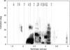 |
Fig. 1 Initial orbit distribution for the test asteroids used in the integrations. The orbit distribution corresponds to an unbiased orbit distribution of known asteroids with different selection criteria for orbits interior and exterior to the 3:1J MMR. |
We made the simplifying assumption that there is no correlation between asteroid orbit and size distributions to the first order because this assumption allows us to assign any physical size to a given test asteroid. The assumption leads to an important caveat with all sets of initial conditions because the size distribution of asteroid families is typically steeper than the background population, and the number of small asteroids belonging to asteroid families is therefore likely to be underestimated. Another caveat is that the assumption is not strictly valid close to resonances where the competition between the size-dependent Yarkovsky drift and the size-independent chaotic diffusion leads to an excess of small asteroids (Guillens et al. 2002). We randomly assigned cosγ = ± 1 to all test asteroids as explained in Sect. 2, and this leads to yet another caveat close to resonances: small asteroids close to resonances should preferentially have an obliquity that would drive them toward the resonance. Imagine a small asteroid on the left side of 3:1J as an example. A retrograde spin would imply that it drifts away from the resonance, but only a small fraction of asteroids are able to cross strong resonances without being ejected from the main belt. Thus a population of small asteroids on the left side of 3:1J should preferentially have prograde rotation, leading to a drift toward the resonance. YORP cycles may revert the direction in some cases, but the overall tendency should be that small asteroids close to a resonance drift toward the resonance. This may slightly affect the estimated fluxes because we generate a random but equal distribution of prograde and retrograde test asteroids close to resonances.
4. Results and discussion
In what follows, we present results using the combined Yarkovsky-YORP model only in Sect. 4.2. That is, in all other sections we only account for the Yarkovsky effect.
4.1. Time-constant Yarkovsky drift for 0.1 km < D < 3 km
We first use set A to assess the sensitivity of the results to different Yarkovsky drift rates. We assigned four different sizes to the test asteroids (0.1 km, 0.3 km, 1.0 km, and 3.0 km) and integrate them for up to 100 Myr with a 10-day time step with the eight planets from Venus through Neptune included as perturbers. We integrated the test asteroids until they were ejected from the solar system or entered the NEO region (q ≤ 1.3 au), and recorded the orbital elements every 10 kyr.
We note that the maximum integration time is dictated by the collisional lifetime in the asteroid belt. The collisional lifetime increases with asteroid size and is about 70 Myr for D = 0.1 km (Bottke et al. 2005). If the integrations spanned much longer than 100 Myr, then we would need to account for the collisional evolution for some parts of the analysis that follows.
Number and fraction of test asteroids achieving q< 1.3 au in the integrations of set A as well as the total number of test asteroids escaping the main belt.
The integrations using set A reveal, as expected, that the number of test asteroids that escape from the main belt dramatically increases when the test asteroid size decreases: the fraction of MBOs escaping in 100 Myr is about 1/37 for D = 3.0 km and about 2/3 for D = 0.1 km (Table 1). If the fractions represented reality, then the main belt and NEO SFDs should be very different. However, the shape of the NEO SFD and the main-belt SFD for D< 1 km (the latter represented by non-saturated craters on Vesta and Gaspra), for example, are in fair agreement with one another. This suggests that there has to exist a mechanism that can slow down the escape of small objects. This also agrees with simplistic estimates from Bottke et al. (2005), who found in their 1D model for the collisional evolution of the main belt that the escape fraction for small objects is not strongly size dependent.
Table 1 also shows that an overwhelming majority of the test asteroids are discarded because the perihelion distance reaches the NEO limit, whereas an ejection from the inner solar system is a rare outcome. In general, an ejection from the inner solar system is typically caused by a close encounter with Jupiter, and the geometry is such that most asteroids need to have q < 1.3 au to have aphelion distance Q >qJ, where qJ is Jupiter’s perihelion distance. Since the integrations presented here are stopped when q = 1.3 au, it is not a surprise that ejections from the inner solar system are rare.
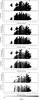 |
Fig. 2 Dynamical stability maps for the main asteroid belt in (a,e,i). The stability is defined as the fraction of test asteroids not escaping in 100 Myr: zero implies that all asteroids have escaped the asteroid belt, and one implies that no asteroids have escaped the asteroid belt (but may have drifted away from the initial location). Test asteroid diameters from top to bottom: 3.0 km, 1.0 km, 0.3 km, and 0.1 km. |
Most of the test particles with D ≥ 0.3 km that escape during the 100 Myr integration were initially close to strong resonances (Fig. 2). For D = 0.1 km the trend is reversed, and regions close to strong resonances appear most stable. The explanation for the apparent discrepancy is that on one hand, test asteroids initially residing close to a resonance and surviving the 100 Myr integration drift away from the resonance. On the other hand, the drift direction for test asteroids initially residing farther from resonances but between two strong resonances is irrelevant because they drift fast enough to reach a resonance on either side of the initial orbit. Hence in a relative sense, the most unstable regions for the smaller asteroids are those midway between strong resonances rather than very close to strong resonances. This explanation raises the question how accurate our model is for small test asteroids that escape in less than 100 Myr and apparently can originate far from the resonances.
Based on the discussion above and in Sect. 2.2.2, it is clear that Yarkovsky-only modeling will not produce realistic escape rates because the obliquity was fixed at cosγ = ± 1 and we did not account for YORP cycles. We return to this issue in Sect. 4.2.
4.1.1. Correlations between size and orbital characteristics of the escaping asteroids
We now make use of the better statistics offered by set B to study whether the orbital characteristics of escaping asteroids varies as a function of size. To maximize the potential difference in the orbital characteristics, we assigned the test asteroids diameters D = 0.1 km and D = 3.0 km. The integration setup was identical to the integrations carried out using set A and described above.
In Fig. 3 we show the fraction of test asteroids escaping through the four different escape-route complexes as a function of their initial semimajor axis. We recall that these results were computed without accounting for the YORP effect. As expected, large test asteroids tend to originate close to the escape route, whereas small test asteroids arrive at the escape route from greater distance. The distributions are nevertheless surprisingly similar considering that the test asteroid diameter (and hence drift rate in semimajor axis) changes by a factor of 30. In other words, the ultimate source regions for asteroids escaping the main belt do not change dramatically as a function of the asteroid size.
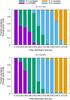 |
Fig. 3 Fraction of test asteroids escaping through four different escape-route complexes as a function of their initial semimajor axes for D = 0.1 km (top) and D = 3.0 km (bottom). |
The last recorded orbital elements for escaping test asteroids with D = 0.1 km and D = 3.0 km show that the locations of the escape routes associated with MMRs and SRs are virtually unaffected by the drift in semimajor axis caused by the Yarkovsky force (Fig. 4). A closer look at the final inclination distributions for escaping test asteroids show that they are also mostly independent of the Yarkovsky drift rate (Fig. 5). Only the inclination distribution corresponding to test asteroids escaping through 7:2J and 9:4J have relatively clear correlations with diameter in that the mode of the distribution increases when the diameter decreases. When comparing the inclination distributions in Figs. 4 and 5, we note that the Hungaria and Phocaea test asteroids were removed before associating test asteroids to the MMRs. For example, the high-inclination group in 7:2J in Fig. 4 belongs to Phocaeas and is not shown in the 7:2J MMR distribution in Fig. 5. The apparent diameter-inclination correlation for Hungarias may be explained by small number statistics. The more likely explanation is that the escaping small test asteroids sample a different part of the initial inclination distribution compared to their larger counterparts because the smaller objects can drift farther in semimajor axis in 100 Myr. Indeed, Fig. 6 shows that the semimajor-axis distribution is markedly different for the two size regimes. We note that the inclination distributions are clearly non-uniform as opposed to the assumption by Bottke et al. (2002) and Greenstreet et al. (2012), for instance.
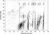 |
Fig. 4 Last recorded a,i of escaping test asteroids for D = 0.1 km (gray) and D = 3.0 km (black). The escape routes coinciding with the MMRs and SRs are identical regardless of the diameter and, hence, the drift rate in semimajor axis of the test asteroid. |
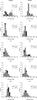 |
Fig. 5 Distributions of last recorded inclinations of test asteroids escaping the asteroid belt for D = 0.1 km and D = 3.0 km. Gray indicates overlapping histograms. |
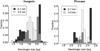 |
Fig. 6 Distributions of last recorded semimajor axes of test asteroids escaping the Hungaria and Phocaea groups for D = 0.1 km and D = 3.0 km. Gray indicates overlapping histograms. The 4:1J MMR is clearly visible as the highest peak in the Hungaria distribution and the left peak in the Phocaea distribution. The middle and right peaks in the Phocaea distribution are the 7:2J and 3:1J MMRs, respectively. |
4.1.2. Overall escape rate of test asteroids
The initial conditions in set B correspond to the distribution of real asteroids with diameters D ≳ 2 km. It is therefore reassuring to see that our nominal Yarkovsky model is producing a nearly constant flux of test asteroids with a diameter of 3 km for the entire 100 Myr integration interval (Fig. 7). The peak at the beginning is due to test asteroids that oscillate between the NEO and MBO regions, enter the NEO region early in the integration, and are thus not integrated further.
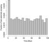 |
Fig. 7 Fraction of test asteroids with D = 3 km escaping as a function of time. The bin size is 5 Myr. |
We integrated the orbits of known NEOs and MBOs with H< 13.5 with the Bulirsch-Stoer (BS) integrator in the MERCURY package (Chambers 1999) to study the oscillation between MBO (q> 1.3 au) and NEO (q< 1.3 au) states. The typical timescale for this oscillation is on the order of tens of thousands of years (Figs. 8 and 9).
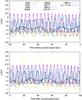 |
Fig. 8 100 kyr backward (top) and forward (bottom) integration of the nine large (H< 13.5) MBOs that enter the NEO region within the next 50 kyr. The integration was carried out with the BS integrator without GR and Yarkovsky. |
Nine known MBOs with H < 13.5 are currently oscillating between MBO and NEO states (Fig. 8). The nine oscillating MBOs spend about a quarter of their time in the NEO region when averaged over 200 kyr. This implies that out of the objects oscillating between NEO and MBO states, about three should be NEOs with H < 13.5 at any given time.
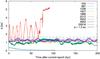 |
Fig. 9 200 kyr integration of the nine largest (H < 13.5) NEOs. The integration was carried out with the BS integrator without GR and Yarkovsky. The red unstable orbit corresponds to the exceptional case of (3552) Don Quixote, a near-Earth comet on a Jupiter-crossing orbit (a ~ 4.2 au, e ~ 0.71, and i ~ 31°), and the blue orbit evolving to small perihelion distance is (2212) Hephaistos, which is predicted to be destroyed in an encounter with the Sun in about 100 kyr. |
There are currently nine NEOs with H< 13.5, and orbital integrations over 200 kyr suggest that three to four of these NEOs are oscillating in the same quasiperiodic manner as the nine current MBOs (Fig. 9). The match is surprisingly good given the small number statistics.
We note that one of the oscillating MBOs may regularly attain an Earth-crossing orbit in the future, thus occasionally increasing the small number of large NEOs on Earth-crossing orbits by 20–100%. There should be a much larger population of smaller objects that oscillate in a similar manner. A fraction of these should periodically be on Earth-crossing orbits. We note that some of these objects may belong to the Kozai class of dynamical behaviour (Milani et al. 1989), which allows for very stable orbits due to the lack of nodal crossings (and hence close encounters) with planets.
For D = 0.1 km the escape rate of test asteroids is no longer flat over 100 Myr (Fig. 10). The explanation for the shape of the distribution is that the initial orbit distribution reflects the distribution of known MBOs with diameters of a few kilometers, but the test asteroids are assigned a much smaller diameter. The escape rate is thus misleading in the beginning of the orbital integration as there are very few large MBOs in the vicinity of the resonances. The semimajor-axis distribution is uniform as long as the drift timescale is short compared to the diffusion timescale. The latter becomes quite short in the vicinity of resonances. Large asteroids, for which the drift timescale is long, therefore show a deficit near the resonances. Figure 10 shows that the flux grows rapidly with time until a maximum is reached, and eventually, the growth turns into a slow decent. We interpret the growth as evidence of the biased distribution of test asteroids in the vicinity of resonances: it takes some time for the gaps to be replenished by test asteroids that start up at larger distances. The slow descent is explained by the fact that our population starts to be thin out toward the end of the integration and thus the escape rate drops. The population would need to be maintained in steady state for the escape flux to remain constant. In reality, therefore, either the population is far less depleted than in the simulation due to YORP, or it is regenerated by collisions, which we did not take into account. We find it unlikely that collisions could support the escape rate discussed here.
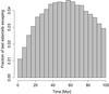 |
Fig. 10 Fraction of test asteroids with D = 0.1 km escaping as a function of time. The bin size is 5 Myr. |
It is interesting to note that the fraction of test asteroids with D = 0.1 km escaping the Hungaria and Phocaea populations is very high: 99.2% of the Hungarias and 96.5% of the Phocaeas had escaped after 100 Myr. These percentages correspond to 1.8% and 3.7% of all test asteroids escaping the main belt. The Hungaria and Phocaea populations are neither dominant nor negligible sources for NEOs when compared to the other source regions (Granvik et al. 2016). Again, we interpret these unrealistically high escape rates as a consequence of not accounting for the YORP effect.
4.1.3. Relative and absolute escape fluxes
Returning to the analysis of set A, we find that the relative importance of the different escape routes is only weakly correlated with size and the statistical uncertainties often overlap (Fig. 11). While the results for D = 3.0 km (and D = 0.1 km with YORP; see Sect. 4.2) may be misleading because of the small number statistics, we used set B to improve the number statistics and found that the relative fluxes are virtually identical to those obtained for set A. An equally good agreement between the relative fluxes was also found for D = 0.1 km (without YORP). The agreement suggests that the lack of small asteroid-family members in the initial conditions has a negligible effect on the relative fluxes when the initial conditions are based on real MBOs with D ≳ 2 km.
The 2:1J MMR is primarily fed from the inside because the 2:1J defines the outer boundary of the main belt. Bottke et al. (2002) concluded that the 2:1J is of negligible importance as a source for NEOs because the vicinity to Jupiter will produce very short-lived NEOs. However, a large amount of material escaping through this MMR works in the other direction, and given that 2:1J appears to be more efficient at smaller sizes, it cannot be ruled out a priori.
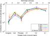 |
Fig. 11 Relative fluxes from the main asteroid belt to the NEO region as a function of escape route or source region as well as test asteroid diameter. |
There is an alternative approach to testing whether escape routes change with the size of a test asteroid: according to Eq. (1), the Yarkovsky drift rate is inversely proportional to the diameter of the test asteroid, that is,  , where a = −1. If the escape routes for the test asteroids are identical regardless of their assigned diameter, then we should find that the fraction of test asteroids escaping in unit time should also be ∝Db with b = a. A fit to the fraction of asteroids entering the NEO region in 100 Myr (Table 1) shows that b = −0.970 ± 0.029, that is, b is statistically indistinguishable from a (Fig. 12). The similarity indicates that each test asteroid that eventually escapes typically does so through the same escape route, regardless of its size and hence Yarkovsky drift rate. That is, it is not common for test asteroids to jump over major resonances as their drift rate increases.
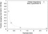 |
Fig. 12 Fraction f of test asteroids escaping the main belt and entering the NEO region as a function of diameter D (crosses). The continuous line is the best-fit function of the form f = cDb with parameters c = 0.0675 ± 0.0043 and b = −0.970 ± 0.029. |
We now consider the absolute flux of asteroids from the asteroid belt to the NEO region and compare with observational evidence. Starting from large asteroids, we have f(D = 3 km) = 0.03 based on integrations of set A, that is, 3% of all MBOs with diameter of 3 km escape in 100 Myr when accounting for Yarkovsky only (also 3% based on set B). Assuming an average geometric albedo pV = 0.14 means that D = 3 km is approximately equivalent to H = 15.4. As of 2016-05-06, there are 118 940 known MBOs, that is, asteroids with perihelion distance q ≥ 1.3 au and semimajor axis a ≤ 4.1 au, with H < 15.4, and the sample can be considered unbiased, as discussed in Sect. 3. Most MBOs in the sample will have H ~ 15.4 because of the SFD slope, and 3568 of these should escape the asteroid belt in 100 Myr and become NEOs according to our model. The average dynamical lifetime for NEOs weighted over source regions is about 4 Myr (Bottke et al. 2002). Our model thus predicts that there should be approximately 143 NEOs with H< 15.4, whereas the observed number is 96 as of 2016-05-06, that is, our model predicts 49% more than is observed. We note that although a new NEO model has recently been presented by Granvik et al. (2016), we here refer to the results in Bottke et al. (2002) for the average lifetimes and fluxes because they were explicitly reported. The use of unpublished numbers derived from the model by Granvik et al. (2016) would not significantly change the results presented here.
To be able to compare the predicted escape-route-specific flux of large asteroids to previous observationally constrained estimates, we need to correct the raw flux of test asteroids escaping the main belt for the skewed distribution of initial conditions close to MMRs and the different completeness limits inside (a < 2.5 au) and outside (a > 2.5 au) 3:1J (cf. Sect. 3). Once this correction has been made, we can compare the relative fluxes obtained from direct integrations of test asteroids with the predictions made by Bottke et al. (2002). The best match should be obtained when the test asteroids’ assigned sizes roughly match the sizes of the asteroids that are the source for the initial orbit distribution. The direct integrations reproduce the fluxes inferred by Bottke et al. (2002) when assigning D = 3 km to the test particles (Table 2).
Relative fluxes, fdirect, of test asteroids with D = 3 km escaping through three main routes compared to predictions by Bottke et al. (2002), fB02.
For smaller sizes the offset between observed and predicted numbers grows larger. Our integrations suggest that 6% of all asteroids with a diameter of 1 km escape in 100 Myr. The known MBO population at this size is not completely known (582 116 MBOs with H< 17.8 known as of 2016-05-06), but we can assume that there are on the order of 106 MBOs with H< 17.8 (Jedicke et al. 2015). This means that about 60 000 should escape in 100 Myr, and that implies a steady-state number of 2400 NEOs with H< 17.8. The most recent estimate for the population is about 1000 (Harris & D’Abramo 2015; Granvik et al. 2016). Our Yarkovsky-only model thus overpredicts the population size by a factor of about 2.
The integrations show that 63% of all asteroids with diameters of 0.1 km escape in 100 Myr when accounting for Yarkovsky only (63% also based on set B). Assuming that there are on the order of 107 MBOs with H< 22.7 (Jedicke et al. 2015), we find that 6 × 10⁶ asteroids escape per 100 Myr, which in turn suggests a steady-state NEO population of about 2.4 × 10⁵. The most recent models agree with each other and predict an order of magnitude fewer (roughly 5 × 10⁴) NEOs with H< 22.7 (Harris & D’Abramo 2015; Granvik et al. 2016). The overprediction is now up to a factor of 5.
An overprediction that systematically increases for smaller asteroids is challenging, if not impossible, to explain by statistics alone. This suggests that some mechanism must be reducing the effective Yarkovsky drift rate and thus the escape of small asteroids from the belt. The most obvious candidate is YORP, which has a larger effect on smaller asteroids and explains the systematically increasing offset with decreasing size.
4.2. Effect of YORP cycles on the net Yarkovsky drift
We now consider YORP more closely as a potential solution to the two apparent contradictions with observations mentioned above, that is, the possibility that asteroids with a diameter of 100 m that escape in just 100 Myr could originate anywhere in the asteroid belt and the overprediction of the flux of small asteroids. We assess the importance and effect of YORP for populating escape routes in the main belt by integrating set A of test asteroids for 100 Myr and simultaneously accounting for YORP. All test asteroids have a diameter of 0.1 km and the initial spin poles are identical to the runs without YORP. The initial rotation rates are uniformly distributed between 1 and 12 h. The density is set to 2.5 g cm-3 and Δ = [C−0.5(A + B)] /C, where A, B, and C are the principal moments of the inertia tensor, follows a Gaussian distribution in the range 0 ≤ Δ ≤ 0.5 with the peak at 0.3 and a standard deviation of 0.1.
In total 285 test asteroids with D = 0.1 km enter the NEO region in 100 Myr when accounting for both Yarkovsky and YORP. We note that this is somewhat less than the 415 for the Yarkovsky-only integration with D = 3 km. The initial and final (a,i) of test asteroids escaping the main belt shows that accounting for YORP cycles reduces the distance from which test asteroids are able to reach a given escape route in 100 Myr (Fig. 13).
The fraction of test asteroids with 0.1 km diameters that are ejected from the main belt in 100 Myr drops from 63% to 2% when accounting for both Yarkovsky and YORP. Again, assuming that there are on the order of 107 MBOs with H< 22.7 (Jedicke et al. 2015), we find that 2 × 10⁵ asteroids escape per 100 Myr, which in turn suggests a steady-state NEO population of 8 × 10³. The latest debiased models predict 5 × 10⁴ NEOs with H< 22.7 (Harris & D’Abramo 2015; Granvik et al. 2016), which suggests that either the MBO population is a factor of 5–6 larger than the above extrapolation suggests, or the YORP modeling employed here is too simplistic.
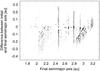 |
Fig. 13 Difference between the initial and final semimajor axis for test asteroids escaping the asteroid belt with (black) and without (gray) YORP modeling. The test asteroids are assigned D = 0.1 km in both cases. |
One possible solution of the mismatch could be the so-called variable YORP mentioned in Sect. 2.2.2 (Bottke et al. 2015), which is based on the idea that the strength of the YORP effect does not only depend on size, but also on time. The reason for the time dependence may originate in YORP’s sensitivity to small-scale surface irregularities (such as crater or boulder fields). If the irregularities change enough on a short timescale, then the YORP strength may also change. An alternative scenario is that the averaged YORP equations for the rotation rate and obliquity are not well determined. Some recent results may even suggest this: Rozitis & Green (2013) claimed that mutual irradiation of small-scale structures may significantly decrease the way in which YORP changes the rotation rate, thus effectively increasing TYORP.
4.3. Characterizing the NEO escape routes
For the remaining part of the analysis we essentially redo the integrations presented in Sect. 4.1, but use a larger number of test asteroids to improve statistics to discuss the NEO escape routes in greater detail. Based on the previous tests, it is clear that the Yarkovsky drift and YORP cycles do not dramatically affect the locations of the escape routes. We therefore focus on test asteroids of a single diameter, D = 0.1 km, and exclude the YORP modeling.
We integrated the entire C set containing 92 449 test asteroids for 100 Myr (or until they were ejected from the solar system or attained q ≤ 1.3 au) with a one-day time step with the eight planets from Mercury through Neptune included as perturbers. We recorded the orbital elements every 10 kyr as before.
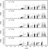 |
Fig. 14 Alternative definitions for the escape routes. The a,i of discarded test asteroids with D = 0.1 km is recorded just before the perihelion distance q reaches the value given in the upper left corner of each subplot. |
At the end of the 100 Myr integration, 21 400 test asteroids were still in the main asteroid belt. A collision with Mars was the end state for 114 test asteroids (0.12% of all test asteroids). The initial orbital elements for Mars-impacting test asteroids typically placed them on Mars-crossing orbits. A close encounter with Jupiter or Saturn ejected 227 test asteroids (0.25%) to either the outer regions of the solar system or completely beyond its limits. The ejected test asteroids were initially on orbits around or beyond the 2:1J MMR, which is responsible for about 96% of the ejections from the inner solar system.
The remaining 70 708 test asteroids (76.5%) escaped the main asteroid belt during the 100 Myr integration and entered the NEO region1. We now focus on the characteristics of this remaining population.
4.3.1. Escape routes from the main asteroid belt and into the NEO region
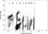 |
Fig. 15 Orbit distribution for test asteroids with q ≃ 1.3 au. |
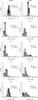 |
Fig. 16 Distributions of initial and last recorded inclinations. Gray indicates overlapping histograms. |
The orbital elements of test asteroids escaping the main asteroid belt depend on how the escape route is defined. Here we have defined a test asteroid escape route using its orbital elements, primarily semimajor axis a and inclination i, at the instant when q ≤ qesc for the first time during the integration. Escape routes associated with MMRs stay nearly constant, as expected, when changing the qesc (Fig. 14). The slanted SRs, on the other hand, change with qesc because the eccentricity e changes. The escape route for a test asteroid may therefore depend on the definition of the escape route. In what follows we use qesc = 1.3 au because this is the formal distinction between NEOs and non-NEOs.
Figure 15 shows the (a,i) distribution for test asteroids that are in the process of entering the NEO region. There is a good match between the essentially empty regions in the (a,i) distribution in the observed main asteroid belt (corresponding to mean-motion and secular resonances; see Fig. 1) and the escape routes from the main asteroid belt to the NEO region. The escape routes associated with MMRs are clearly identifiable as test asteroids extended in inclination and concentrated in semimajor axis at the time of entering the NEO region (Fig. 15). Most of the MMRs in the main belt are well known, but the non-negligible contribution from the 1:2E, 5:1J, and 2:5E MMRs was unexpected. The source for test asteroids escaping through these MMRs is the Hungaria population, which primarily resides exterior to the 2:5E MMR.
Neglecting the vertical concentrations of test asteroids escaping through MMRs, we are left with a number of curved and slanted concentrations of test asteroids that can be identified with secular resonances, most notably the ν6 with approximate coordinates for the cluster centered at a ~ 2.1 au and i ~ 5°. We also find putative identifications to other linear and nonlinear SRs by comparing the test asteroids’ osculating orbital elements to published maps of SRs based on proper elements (e.g., Milani & Knežević 1994; Michel et al. 1998; Milani et al. 2010): the “wings” extending from the 4:1J MMR caused by the ν16 at high inclinations and the ν5 at slightly lower inclinations, the U-shaped ν6 between the 3:1J and 5:2J MMRs (2.51 au <a< 2.78 au), and the slanted z2 between the 5:2J and 2:1J MMRs (2.84 au <a< 3.15 au).
We note that maps of SRs based on analytical proper elements (e.g., Milani & Knežević 1994) are useful in the qualitative sense, but synthetic elements are much more accurate and therefore preferable for assigning a specific asteroid to a certain resonance (Knežević et al. 2002). However, here we are mainly concerned with providing approximate classifications to separate between different source regions. Furthermore, our putative identifications are based on maps in (aprop, iprop) space where eprop is held constant and typically attains values up to 0.25. The escaping test asteroids’ osculating elements, on the other hand, are constrained by the requirement that a(1−e) = 1.3 au, which implies that 0 <e ≲ 0.68 when 1.3 au <a< 4.1 au. So there are no accurate maps for 0.25 <e< 0.68 and accurate SR maps for q = 1.3 au exist only for 1.3 au ≲ a ≲ 1.7 au. All our candidate identifications are for SRs with a> 1.8 au and are thus approximate. The lack of maps of secular resonances at higher eccentricities is explained by the fact that their calculation is extremely challenging in the presence of close planetary encounters, and higher eccentricities imply orbits that cross the orbits of the terrestrial planets. Maps of SRs for planet-crossing orbits could potentially be computed using the secular theory for NEO orbits developed by Gronchi & Milani (2001) and Gronchi (2002).
SRs are able to modify inclinations over time (e.g., Froeschle & Scholl 1986), whereas MMRs should not affect the inclinations in the first approximation. Comparing the initial and final inclination distributions of escaping test asteroids, we find that the distributions for the 8:3J, 5:2J and 7:3J MMRs are virtually constant (Fig. 16). The orbits of test asteroids escaping through ν6 and 3:1J are systematically shifted to higher inclinations, those escaping through 7:2J on high (low) inclinations systematically shift to lower (higher) inclinations, and those escaping through 9:4J are systematically shifted to lower inclination. The explanation for the changing inclinations in MMRs are the secular resonances embedded in them (Moons & Morbidelli 1995). The 3:1J MMR is a good example that has been numerically verified in the past (Morbidelli & Moons 1995), and the inclination effects in 7:2J are caused by ν6. The width of the inclination distributions for Phocaeas and Hungarias increases over time, which, particularly for the latter, implies that they cannot explain missing NEOs with 20° ≲ i ≲ 30° without also affecting the inclination distribution exterior to that range of values.
4.3.2. Relation between escape route and test asteroid source region
Most of the test asteroids escaping through any given escape route, for example, the ν6, were initially adjacent to that escape route. This makes sense because even test asteroids with diameters of 100 m typically drift too slowly in semimajor axis to cross powerful resonances without becoming ejected from the main asteroid belt.
Although the fraction of test asteroids that are able to cross strong resonances is small, the integrations show that they do exist. For instance, Fig. 17 shows the initial orbital distribution of test asteroids (black) that will cross the 3:1J MMR before eventually escaping through ν6 as well as their orbital elements at the time of the escape (gray). About 1.5% of all test asteroids that escape through ν6 have initially had a> 2.51 au, that is, they have had to cross the 3:1J MMR. The fraction of test asteroids crossing neighboring major resonances is substantially smaller for test asteroids escaping through major MMRs such as 3:1J, 5:2J, 9:4J, and 2:1J. We note that the fraction of test asteroids able to cross major resonances will be reduced compared to the values shown here if accounting for YORP cycles because the net drift rates in semimajor axis will be lower.
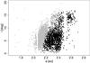 |
Fig. 17 Orbital elements corresponding to the initial conditions (black) and situation at the time of escape (gray) for test asteroids escaping through ν6. |
5. Conclusions
We have carried out extensive orbital integrations for a representative set of main-belt objects to locate escape routes into the near-Earth space. Our global approach allowed us to find all important source regions for NEOs, and it provided a detailed and realistic (a,i) distribution for asteroids that are about to enter the NEO region.
The escape rate of large test asteroids (D ≳ 3 km) is about 50% higher than the observed flux of NEOs when only accounting for the drift in semimajor axis caused by the Yarkovsky effect, and the difference between predicted and observed flux grows larger for smaller asteroids. The predicted and observationally constrained escape rates can be reconciled by accounting for the changes in the Yarkovsky drift rate caused by YORP cycling.
The escape routes are unaffected when the drift rate changes, but the source regions depend on the drift rate (and thus the size of the asteroid). The source regions and orbit distributions for test asteroids entering the NEO region were used to construct a new debiased model of the NEO population (Granvik et al. 2016).
The initial and final orbital elements are available at http://www.iki.fi/mgranvik/data/Granvik+_2017_A&A
Acknowledgments
We thank Andrea Milani for the thorough referee report that helped us improve the paper. M.G. was supported by grants #137853 and #299543 from the Academy of Finland and D.V. by grant GA13-01308S from the Czech Science Foundation. Computing resources for this study were provided by CSC – IT Center for Science and the Finnish Grid Infrastructure.
References
- Bertotti, B., Farinella, P., & Vokrouhlický, D. 2003, in Physics of the Solar System (New York: Kluwer Academic Publishers) [Google Scholar]
- Bottke, W. F., Jedicke, R., Morbidelli, A., Petit, J.-M., & Gladman, B. 2000, Science, 288, 2190 [NASA ADS] [CrossRef] [PubMed] [Google Scholar]
- Bottke, W. F., Morbidelli, A., Jedicke, R., et al. 2002, Icarus, 156, 399 [NASA ADS] [CrossRef] [Google Scholar]
- Bottke, W. F., Durda, D. D., Nesvorný, D., et al. 2005, Icarus, 179, 63 [NASA ADS] [CrossRef] [Google Scholar]
- Bottke, W., Vokrouhlický, D., Rubincam, D., & Nesvorný, D. 2006, Ann. Rev. Earth Planet. Sci., 34, 157 [Google Scholar]
- Bottke, W. F., Vokrouhlický, D., Walsh, K. J., et al. 2015, Icarus, 247, 191 [NASA ADS] [CrossRef] [Google Scholar]
- Breiter, S., Nesvorný, D., & Vokrouhlický, D. 2005, AJ, 130, 1267 [NASA ADS] [CrossRef] [Google Scholar]
- Breiter, S., Bartczak, P., Czekaj, M., Oczujda, B., & D., V. 2009, ApJ, 507, 1073 [Google Scholar]
- Breiter, S., Rożek, A., & Vokrouhlický, D. 2011, MNRAS, 417, 2478 [NASA ADS] [CrossRef] [Google Scholar]
- Chambers, J. E. 1999, MNRAS, 304, 793 [NASA ADS] [CrossRef] [MathSciNet] [Google Scholar]
- Cicalò, S., & Scheeres, D. 2010, Mech. Dyn. Astron., 106, 301 [NASA ADS] [CrossRef] [Google Scholar]
- Cordeiro, R., Gomes, R., & Vieira Martins, R. 1997, Mech. Dyn. Astron., 65, 407 [Google Scholar]
- Delbò, M., Dell’Oro, A., Harris, A., Mottola, S., & Mueller, M. 2007, Icarus, 90, 236 [CrossRef] [Google Scholar]
- Denneau, L., Jedicke, R., Fitzsimmons, A., et al. 2015, Icarus, 245, 1 [NASA ADS] [CrossRef] [Google Scholar]
- Farinella, P., Vokrouhlický, D., & Hartman, W. 1998, Icarus, 132, 378 [NASA ADS] [CrossRef] [Google Scholar]
- Farnocchia, D., Chesley, S. R., Vokrouhlický, D., et al. 2013, Icarus, 224, 1 [NASA ADS] [CrossRef] [Google Scholar]
- Froeschle, C., & Scholl, H. 1986, A&A, 166, 326 [NASA ADS] [Google Scholar]
- Gladman, B. J., Migliorini, F., Morbidelli, A., et al. 1997, Science, 277, 197 [NASA ADS] [CrossRef] [Google Scholar]
- Golubov, O., & Krugly, Y. 2012, ApJ, 752, L11 [NASA ADS] [CrossRef] [Google Scholar]
- Granvik, M., Morbidelli, A., Jedicke, R., et al. 2016, Nature, 530, 303 [Google Scholar]
- Greenstreet, S., Ngo, H., & Gladman, B. 2012, Icarus, 217, 355 [NASA ADS] [CrossRef] [Google Scholar]
- Gronchi, G. F. 2002, Mech. Dyn. Astron., 83, 97 [NASA ADS] [CrossRef] [Google Scholar]
- Gronchi, G. F., & Milani, A. 2001, Icarus, 152, 58 [NASA ADS] [CrossRef] [Google Scholar]
- Guillens, S., Vieira Martins, R., & Gomes, R. 2002, AJ, 124, 2322 [NASA ADS] [CrossRef] [Google Scholar]
- Hanuš, J., Ďurech, J., Brož, M., et al. 2011, A&A, 530, A134 [NASA ADS] [CrossRef] [EDP Sciences] [Google Scholar]
- Hanuš, J., Ďurech, J., Brož, M., et al. 2013, A&A, 551, A67 [NASA ADS] [CrossRef] [EDP Sciences] [Google Scholar]
- Harris, A. W., & D’Abramo, G. 2015, Icarus, 257, 302 [NASA ADS] [CrossRef] [Google Scholar]
- Jedicke, R., Granvik, M., Micheli, M., et al. 2015, in Surveys, Astrometric Follow-Up, and Population Statistics, eds. P. Michel, F. E. DeMeo, & W. F. Bottke (Tucson: University of Arizona Press), 795 [Google Scholar]
- Knežević, Z., Lemaître, A., & Milani, A. 2002, in Asteroids III, eds. W. F. Bottke, Jr., A. Cellino, P. Paolicchi, & R. P. Binzel (Tucson: University of Arizona Press), 603 [Google Scholar]
- Levison, H. F., & Duncan, M. J. 1994, Icarus, 108, 18 [NASA ADS] [CrossRef] [Google Scholar]
- McFadden, L.-A., Tholen, D. J., & Veeder, G. J. 1989, in Asteroids II, eds. R. P. Binzel, T. Gehrels, & M. S. Matthews (Tucson: University of Arizona Press), 442 [Google Scholar]
- Michel, P., Froeschlé, C., & Farinella, P. 1998, Mech. Dyn. Astron., 69, 133 [NASA ADS] [CrossRef] [Google Scholar]
- Mikkola, S. 1997, Cel. Mech. Dyn. Astron., 68, 249 [Google Scholar]
- Milani, A., & Knežević, Z. 1994, Icarus, 107, 219 [NASA ADS] [CrossRef] [Google Scholar]
- Milani, A., Carpino, M., Hahn, G., & Nobili, A. M. 1989, Icarus, 78, 212 [NASA ADS] [CrossRef] [Google Scholar]
- Milani, A., Knežević, Z., Novaković, B., & Cellino, A. 2010, Icarus, 207, 769 [NASA ADS] [CrossRef] [Google Scholar]
- Moons, M., & Morbidelli, A. 1995, Icarus, 114, 33 [NASA ADS] [CrossRef] [Google Scholar]
- Morbidelli, A., & Moons, M. 1995, Icarus, 115, 60 [NASA ADS] [CrossRef] [Google Scholar]
- Morbidelli, A., & Vokrouhlický, D. 2003, Icarus, 163, 120 [NASA ADS] [CrossRef] [Google Scholar]
- Morbidelli, A., Bottke, W. F., Jr., Froeschlé, C., & Michel, P. 2002, in Asteroids III, eds. W. F. Bottke, Jr., A. Cellino, P. Paolicchi, & R. P. Binzel (Tucson: University of Arizona Press), 409 [Google Scholar]
- Nesvorný, D., & Vokrouhlický, D. 2006, AJ, 132, 1950 [NASA ADS] [CrossRef] [Google Scholar]
- Nesvorný, D., Jenniskens, P., Levison, H., Bottke, W., Vokrouhlický, D., & Gounelle, M. 2010, ApJ, 713, 816 [NASA ADS] [CrossRef] [Google Scholar]
- Nobili, A.-M., & Roxburgh, I. 1986, in Relativity in celestial mechanics and astrometry, eds. J. Kovalevsky, & V. Brumberg (Dordrecht: D. Reidel Publishing), 105 [Google Scholar]
- Nobili, A.-M., Milani, A., & Carpino, M. 1989, A&A, 210, 313 [NASA ADS] [Google Scholar]
- Pravec, P., Harris, A. W., & Michalowski, T. 2002, in Asteroids III, eds. W. Bottke, A. Cellino, P. Paolicchi, & R. P. Binzel (Tucson: University of Arizona Press), 113 [Google Scholar]
- Pravec, P., Harris, A. W., Scheirich, P., et al. 2005, Icarus, 173, 108 [NASA ADS] [CrossRef] [Google Scholar]
- Pravec, P., Vokrouhlický, D., Polishook, D., et al. 2010, Nature, 466, 1085 [NASA ADS] [CrossRef] [Google Scholar]
- Rozitis, B., & Green, S. F. 2012, MNRAS, 423, 367 [NASA ADS] [CrossRef] [Google Scholar]
- Rozitis, B., & Green, S. F. 2013, MNRAS, 433, 603 [NASA ADS] [CrossRef] [Google Scholar]
- Rubincam, D. P. 2000, Icarus, 148, 2 [NASA ADS] [CrossRef] [Google Scholar]
- Saha, P., & Tremaine, S. 1994, AJ, 108, 1962 [NASA ADS] [CrossRef] [Google Scholar]
- Statler, T. 2009, Icarus, 202, 502 [NASA ADS] [CrossRef] [Google Scholar]
- Strom, R. G., Renu, M., Xiao, Z.-Y., et al. 2015, RA&A, 15, 407 [Google Scholar]
- Čapek, D., & Vokrouhlický, D. 2004, Icarus, 172, 526 [NASA ADS] [CrossRef] [Google Scholar]
- Vokrouhlický, D. 1998, A&A, 335, 1093 [NASA ADS] [Google Scholar]
- Vokrouhlický, D. 1999, A&A, 344, 362 [NASA ADS] [Google Scholar]
- Vokrouhlický, D., & Nesvorný, D. 2008, AJ, 136, 280 [NASA ADS] [CrossRef] [Google Scholar]
- Vokrouhlický, D., Nesvorný, D., & Bottke, W. F. 2006a, Icarus, 184, 1 [NASA ADS] [CrossRef] [Google Scholar]
- Vokrouhlický, D., Brož, M., Bottke, W., Nesvorný, D., & Morbidelli, A. 2006b, Icarus, 182, 118 [NASA ADS] [CrossRef] [Google Scholar]
- Vokrouhlický, D., Breiter, S., Nesvorný, D., & Bottke, W. F. 2007, Icarus, 191, 636 [NASA ADS] [CrossRef] [Google Scholar]
- Vokrouhlický, D., Bottke, W. F., Chesley, S. R., Scheeres, D. J., & Statler, T. S. 2015, in Asteroids IV, eds. P. Michel, F. E. DeMeo, & W. F. Bottke (Tucson: University of Arizona Press), 509 [Google Scholar]
- Will, C. 1993, in Theory and Experiment in Gravitational Physics (Cambridge: Cambridge University Press) [Google Scholar]
- Wisdom, J. 1982, AJ, 87, 577 [NASA ADS] [CrossRef] [Google Scholar]
- Wisdom, J. 1983, Icarus, 56, 51 [NASA ADS] [CrossRef] [Google Scholar]
All Tables
Number and fraction of test asteroids achieving q< 1.3 au in the integrations of set A as well as the total number of test asteroids escaping the main belt.
Relative fluxes, fdirect, of test asteroids with D = 3 km escaping through three main routes compared to predictions by Bottke et al. (2002), fB02.
All Figures
|
Fig. 1 Initial orbit distribution for the test asteroids used in the integrations. The orbit distribution corresponds to an unbiased orbit distribution of known asteroids with different selection criteria for orbits interior and exterior to the 3:1J MMR. |
| In the text | |
|
Fig. 2 Dynamical stability maps for the main asteroid belt in (a,e,i). The stability is defined as the fraction of test asteroids not escaping in 100 Myr: zero implies that all asteroids have escaped the asteroid belt, and one implies that no asteroids have escaped the asteroid belt (but may have drifted away from the initial location). Test asteroid diameters from top to bottom: 3.0 km, 1.0 km, 0.3 km, and 0.1 km. |
| In the text | |
|
Fig. 3 Fraction of test asteroids escaping through four different escape-route complexes as a function of their initial semimajor axes for D = 0.1 km (top) and D = 3.0 km (bottom). |
| In the text | |
|
Fig. 4 Last recorded a,i of escaping test asteroids for D = 0.1 km (gray) and D = 3.0 km (black). The escape routes coinciding with the MMRs and SRs are identical regardless of the diameter and, hence, the drift rate in semimajor axis of the test asteroid. |
| In the text | |
|
Fig. 5 Distributions of last recorded inclinations of test asteroids escaping the asteroid belt for D = 0.1 km and D = 3.0 km. Gray indicates overlapping histograms. |
| In the text | |
|
Fig. 6 Distributions of last recorded semimajor axes of test asteroids escaping the Hungaria and Phocaea groups for D = 0.1 km and D = 3.0 km. Gray indicates overlapping histograms. The 4:1J MMR is clearly visible as the highest peak in the Hungaria distribution and the left peak in the Phocaea distribution. The middle and right peaks in the Phocaea distribution are the 7:2J and 3:1J MMRs, respectively. |
| In the text | |
|
Fig. 7 Fraction of test asteroids with D = 3 km escaping as a function of time. The bin size is 5 Myr. |
| In the text | |
|
Fig. 8 100 kyr backward (top) and forward (bottom) integration of the nine large (H< 13.5) MBOs that enter the NEO region within the next 50 kyr. The integration was carried out with the BS integrator without GR and Yarkovsky. |
| In the text | |
|
Fig. 9 200 kyr integration of the nine largest (H < 13.5) NEOs. The integration was carried out with the BS integrator without GR and Yarkovsky. The red unstable orbit corresponds to the exceptional case of (3552) Don Quixote, a near-Earth comet on a Jupiter-crossing orbit (a ~ 4.2 au, e ~ 0.71, and i ~ 31°), and the blue orbit evolving to small perihelion distance is (2212) Hephaistos, which is predicted to be destroyed in an encounter with the Sun in about 100 kyr. |
| In the text | |
|
Fig. 10 Fraction of test asteroids with D = 0.1 km escaping as a function of time. The bin size is 5 Myr. |
| In the text | |
|
Fig. 11 Relative fluxes from the main asteroid belt to the NEO region as a function of escape route or source region as well as test asteroid diameter. |
| In the text | |
|
Fig. 12 Fraction f of test asteroids escaping the main belt and entering the NEO region as a function of diameter D (crosses). The continuous line is the best-fit function of the form f = cDb with parameters c = 0.0675 ± 0.0043 and b = −0.970 ± 0.029. |
| In the text | |
|
Fig. 13 Difference between the initial and final semimajor axis for test asteroids escaping the asteroid belt with (black) and without (gray) YORP modeling. The test asteroids are assigned D = 0.1 km in both cases. |
| In the text | |
|
Fig. 14 Alternative definitions for the escape routes. The a,i of discarded test asteroids with D = 0.1 km is recorded just before the perihelion distance q reaches the value given in the upper left corner of each subplot. |
| In the text | |
|
Fig. 15 Orbit distribution for test asteroids with q ≃ 1.3 au. |
| In the text | |
|
Fig. 16 Distributions of initial and last recorded inclinations. Gray indicates overlapping histograms. |
| In the text | |
|
Fig. 17 Orbital elements corresponding to the initial conditions (black) and situation at the time of escape (gray) for test asteroids escaping through ν6. |
| In the text | |
Current usage metrics show cumulative count of Article Views (full-text article views including HTML views, PDF and ePub downloads, according to the available data) and Abstracts Views on Vision4Press platform.
Data correspond to usage on the plateform after 2015. The current usage metrics is available 48-96 hours after online publication and is updated daily on week days.
Initial download of the metrics may take a while.