| Issue |
A&A
Volume 597, January 2017
|
|
|---|---|---|
| Article Number | A40 | |
| Number of page(s) | 13 | |
| Section | Interstellar and circumstellar matter | |
| DOI | https://doi.org/10.1051/0004-6361/201629506 | |
| Published online | 20 December 2016 | |
History of the solar-type protostar IRAS 16293–2422 as told by the cyanopolyynes
1 Univ. Grenoble Alpes,
CNRS, IPAG, 38000 Grenoble, France
e-mail: This email address is being protected from spambots. You need JavaScript enabled to view it.
;This email address is being protected from spambots. You need JavaScript enabled to view it.
2 University of AL-Muthanna, College of
Science, Physics Department, 38028
AL-Muthanna,
Iraq
3 University College
London, Gower
Street, London
WC1E 6BT,
UK
4 Dipartimento di
Chimica, Biologia e
Biotecnologie, 06123
Perugia,
Italy
5 Université de Toulouse,
UPS-OMP, IRAP, 31400
Toulouse,
France
6 CNRS, IRAP, 9 Av. Colonel Roche, BP 44346, 31028
Toulouse Cedex 4,
France
7 LOMC – UMR 6294, CNRS-Université du
Havre, 25 rue Philippe
Lebon, BP 1123,
76063
Le Havre,
France
8 Instituto de Astronomia, Geofísica e
Ciencias Atmosféricas, Universidade de São Paulo, 05508-090
São Paulo, SP, Brazil
Received:
9
August
2016
Accepted:
22
September
2016
Abstract
Context. Cyanopolyynes are chains of carbon atoms with an atom of hydrogen and a CN group on either side. They are detected almost everywhere in the interstellar medium (ISM), as well as in comets. In the past, they have been used to constrain the age of some molecular clouds, since their abundance is predicted to be a strong function of time. Finally, cyanopolyynes can potentially contain a large portion of molecular carbon.
Aims. We present an extensive study of the cyanopolyynes distribution in the solar-type protostar IRAS 16293-2422. The goals are (i) to obtain a census of the cyanopolyynes in this source and of their isotopologues; (ii) to derive how their abundance varies across the protostar envelope; and (iii) to obtain constraints on the history of IRAS 16293-2422 by comparing the observations with the predictions of a chemical model.
Methods. We analysed the data from the IRAM-30 m unbiased millimeter and submillimeter spectral survey towards IRAS 16293-2422 named TIMASSS. The derived spectral line energy distribution (SLED) of each detected cyanopolyyne was compared with the predictions from the radiative transfer code GRenoble Analysis of Protostellar Envelope Spectra (GRAPES) to derive the cyanopolyyne abundances across the envelope of IRAS 16293-2422. Finally, the derived abundances were compared with the predictions of the chemical model UCL_CHEM.
Results. We detect several lines from cyanoacetylene (HC3N) and cyanodiacetylene (HC5N), and report the first detection of deuterated cyanoacetylene, DC3N, in a solar-type protostar. We found that the HC3N abundance is roughly constant (~1.3 × 10⁻¹¹) in the outer cold envelope of IRAS 16293-2422, and it increases by about a factor 100 in the inner region where the dust temperature exceeds 80 K, namely when the volcano ice desorption is predicted to occur. The HC5N has an abundance similar to HC3N in the outer envelope and about a factor of ten lower in the inner region. The comparison with the chemical model predictions provides constraints on the oxygen and carbon gaseous abundance in the outer envelope and, most importantly, on the age of the source. The HC3N abundance derived in the inner region, and where the increase occurs, also provide strong constraints on the time taken for the dust to warm up to 80 K, which has to be shorter than ~103−104 yr. Finally, the cyanoacetylene deuteration is about 50% in the outer envelope and ≤5% in the warm inner region. The relatively low deuteration in the warm region suggests that we are witnessing a fossil of the HC3N abundantly formed in the tenuous phase of the pre-collapse and then frozen into the grain mantles at a later phase.
Conclusions. The accurate analysis of the cyanopolyynes in IRAS 16293-2422 unveils an important part of its past story. It tells us that IRAS 16293-2422 underwent a relatively fast (≤105 yr) collapse and a very fast (≤103−104 yr) warming up of the cold material to 80 K.
Key words: astrochemistry / ISM: abundances / ISM: individual objects: IRAS 16293-2422
© ESO, 2016
1. Introduction
Cyanopolyynes, H-C2n-CN, are linear chains of 2n carbons bonded at the two extremities with a hydrogen atom and a CN group, respectively. They seem to be ubiquitous in the interstellar medium (ISM), as they have been detected in various environments, from molecular clouds to late-type carbon-rich asymptotic giant branch (AGB) stars. The detection of the largest cyanopolyyne, HC11N, has been reported and then dismissed in the molecular cloud TMC-1 (Bell et al. 1997; Loomis et al. 2016), which shows an anomalously large abundance of cyanopolyynes with respect to other molecular clouds. Curiously enough, in star-forming regions, only relatively short chains have been reported in the literature so far, up to HC7N, in dense cold cores and warm carbon-chain chemistry (WCCC) sources (e.g. Sakai et al. 2008; Cordiner et al. 2012; Friesen et al. 2013). For many years, cyanopolyynes have been suspected to be possible steps in the synthesis of simple amino acids (e.g. Brack 1998). More recently, the rich N-chemistry leading to large cyanopolyynes chains observed in Titan has renewed the interest in this family of molecules, as Titan is claimed to be a possible analogue of the early Earth (Lunine 2009). An important property of cyanopolyynes that is particularly relevant for astrobiological purposes is that they are more stable and robust against the harsh interstellar environment compared to their monomer, and hence they may better resist the exposure to UV and cosmic rays (Clarke & Ferris 1995). Very recent observations towards the comet 67P/Churyumov-Gerasimenko by Rosetta seem to support the idea that cyanide polymers, and, by analogy, cyanopolyynes, are abundant on the comet’s surface (Goesmann et al. 2015).
Regardless of the role of cyanopolyynes in prebiotic chemistry, when trapped in interstellar ices, they can certainly carry large quantities of carbon atoms. It is, therefore, of interest to understand in detail their formation, carbon chain accretion, and evolution in solar-like star-forming regions. The goal of this article is to provide the first census of cyanopolyynes in a solar-like protostar. To this end, we used the 3−1 mm unbiased spectral survey TIMASSS (Sect. 3) towards the well-studied protostar IRAS 16293-2422 (Sect. 2), to derive the abundance across the envelope and hot corino of HC3N, HC5N and their respective isotopologues (Sect. 4). The measured abundance profiles provide us with constraints on the formation routes of these species (Sect. 5). Section 6 discusses the implications of the analysis, and Sect. 7 summarises our conclusions.
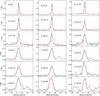 |
Fig. 1 Observed spectra of the detected lines of HC3N. The red curves show the Gaussian fits. The temperature is a main-beam antenna temperature. |
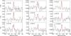 |
Fig. 2 Observed spectra of the detected lines of HC5N. The red curves show the Gaussian fits. The temperature is a main-beam antenna temperature. |
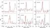 |
Fig. 3 Observed spectra of the detected lines of DC3N. The red curves show the Gaussian fits. The temperature is a main-beam antenna temperature. |
2. Source description
IRAS 16293-2422 (hereafter IRAS 16293) is a solar-type Class 0 protostar in the ρ Ophiuchus star-forming region, at a distance of 120 pc (Loinard et al. 2008). It has a bolometric luminosity of 22 L⊙ (Crimier et al. 2010). Given its proximity and brightness, it has been the target of numerous studies that have reconstructed its physical and chemical structure. Briefly, IRAS 16293 has a large envelope that extends up to ~6000 AU and that surrounds two sources, named I16293-A and I16293-B in the literature, separated by ~5″ (~600 AU; Wootten 1989; Mundy et al. 1992). I16293-A sizes are ~1″, whereas I16293-B is unresolved at a scale of ~0.4″ (Zapata et al. 2013). I16293-A itself is composed of at least two sources, each one emitting a molecular outflow (Mizuno et al. 1990; Loinard et al. 2013). I16293-B possesses a very compact outflow (Loinard et al. 2013) and is surrounded by infalling gas (Pineda et al. 2012; Zapata et al. 2013). From a chemical point of view, IRAS 16293 can be considered as composed of an outer envelope, characterised by low molecular abundances, and a hot corino, where the abundance of many molecules increases by orders of magnitude (e.g. Ceccarelli et al. 2000; Schöier et al. 2002; Cazaux et al. 2003; Jaber et al. 2014). The transition between the two regions is presumed to occur at ~100 K, which is the sublimation temperature of the icy grain mantles.
3. Data set
3.1. Observations
We used data from The IRAS 16293 Millimeter And Submillimeter Spectral Survey (TIMASSS; Caux et al. 2011). Briefly, the survey covers the 80−280 GHz frequency interval and it has been obtained at the IRAM-30 m during the period January 2004 to August 2006 (~200 h). Details on the data reduction and calibration can be found in Caux et al. (2011). We recall here the main features that are relevant for this work. The telescope beam depends on the frequency and varies between 9′′ and 30′′. The spectral resolution varies between 0.3 and 1.25 MHz, corresponding to velocity resolutions between 0.51 and 2.25 km s-1. The achieved rms ranges from 4 to 17 mK. We note that it is given in a 1.5 km s-1 bin for observations taken with a velocity resolution ≤1.5 km s-1, and in the resolution bin for higher velocity resolutions. The observations are centered on I16293-B at α(2000.0) = 16h32m22s.6 and δ(2000.0) = −24°28′33′′. We note that the I16293-A and I16293-B components are both inside the beam of the observations at all frequencies.
3.2. Species identification
We searched for the lines of cyanopolyynes and their isotopologues using the spectroscopic databases Jet Propulsion Laboratory (JPL; Pickett et al. 1998) and the Cologne Database for Molecular Spectroscopy (CDMS; Müller et al. 2005). We then used the package CASSIS (Centre d’Analyse Scientifique de Spectres Instrumentaux et Synthétiques)1 to fit a Gaussian to the lines. For the line identification we adopted the following criteria:
-
The line is detected with more than 3σ in the integrated line intensity.
-
The line is not blended with other molecular lines.
-
The line intensity is compatible with the spectral line energy distribution (SLED): since cyanopolyyynes are linear molecules, their SLED is a smooth curve, so that lines are discarded when their intensities are out of the SLED defined by the majority of the lines, as shown in Fig. A.1.
-
The full width at half-maximum (FWHM) of the line is similar to that of the other cyanopolyyne lines with a similar upper level energy. In practice, a posteriori the FWHM is about 2 km s-1 for lines with J ≤ 12 and increases to 6–7 km s-1 for J = 22−30 lines.
-
The line rest velocity VLRS does not differ by more than 0.5 km s-1 from the VLRS of the other cyanopolyyne lines.
The first two criteria lead to the detection of 18 lines of HC3N (from J = 9−8 to J = 30−29), 9 lines of HC5N (from J = 31−30 to J = 39−38), and the detection of 6 lines of DC3N (from J = 10−9 to J = 17−16). The full list of detected lines with their spectroscopic parameters is reported in Table 1. All the spectra are shown in Figs. 1−3 for HC3N, HC5N, and DC3N, respectively. We did not detect any line from the 13C isotopologues of HC3N.
We applied the remaining three criteria and then discarded four HC3N lines (at 109.173, 245.606, 254.699, and 263.792 GHz) that had calibration problems (Caux et al. 2011) and/or were blended with unidentified species (see Fig. A.1). Similarly, one HC5N line (at 95.850 GHz) was discarded because of its abnormal values of the intensity, FWHM, and velocity compared to the rest of the lines (see Table 1). Finally, one DC3N (at 135.083 GHz) is considered as tentatively detected.
In summary, we clearly detected HC3N, HC5N, and DC3N, for which 14, 8, and 6 lines were identified following the five criteria above. We did not detect any 13C isotopologue of HC3N, nor cyanopolyynes larger than HC5N.
Parameters of the detected cyanopolyynes lines.
4. Line modelling
4.1. Model description
As in our previous work (Jaber et al. 2014), we used the package GRAPES (GRenoble Analysis of Protostellar Envelope Spectra), which is based on the code described in Ceccarelli et al. (1996, 2003), to interpret the SLED of the detected cyanopolyynes. Briefly, GRAPES computes the SLED from a spherical infalling envelope for a given density and temperature structure. The code uses the beta escape probability formalism to locally solve the level population statistical equilibrium equations and consistently computes each line optical depth by integrating it over the solid angle at each point of the envelope. The predicted line flux is then integrated over the whole envelope after convolution with the telescope beam. The abundance X (with respect to H2) of the considered species is assumed to vary as a function of the radius with a power law α in the cold part of the envelope, and as a jump to a new abundance in the warm part, corresponding to the sublimation of ices (e.g. Caselli & Ceccarelli 2012). The transition between the two regions is set by the dust temperature, to simulate the sublimation of the ice mantles, and occurs at Tjump.
The abundance is therefore given by 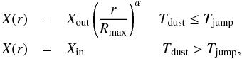 (1)where Rmax represents the largest radius of the envelope. We here used the physical structure of the IRAS 16293 envelope derived by Crimier et al. (2010), where the maximum radius is 1 × 1017 cm.
We carried out non-local thermal equilibrium (NLTE) calculations for all detected species. We used the collisional coefficients for HC3N computed by Faure et al. (2016). For DC3N collisional coefficients, we assumed the same as those of HC3N. Finally, the collisional coefficients for HC5N have been computed by Lique et al. (in prep.). Briefly, HC5N rate coefficients were extrapolated from HCN (Ben Abdallah et al. 2012) and HC3N (Wernli et al. 2007) considering that the cyanopolyyne rate coefficients are proportional to the size of the molecules as first suggested by Snell et al. (1981). However, to improve the accuracy of the estimation, we considered scaling factors that also depend on the transition and the temperature. Hence, the ratio of HC3N to HCN rate coefficients was also used to evaluate the HC5N coefficients as follows: ![Mathematical equation: \begin{eqnarray} k_{HC_5N}(T) = k_{\rm HC_3N}(T) * \left[\frac{1}{2} + \frac{1}{2} \frac{k_{\rm HC_3N}(T)}{k_{HCN}(T)}\right] \cdot \label{eq:2} \end{eqnarray}](/articles/aa/full_html/2017/01/aa29506-16/aa29506-16-eq52.png) (2)We assumed the Boltzmann value for the ortho-to-para ratio of H2. Finally, we note that the disadvantage of GRAPES, namely its inability to compute the emission separately for the two sources I16293-A and I16293-B (Jaber et al. 2014), can be neglected here because previous interferometric observations by Chandler et al. (2005) and Jørgensen et al. (2011) have demonstrated that the cyanopolyyne line emission arises from source I16293-A, as also found by the analysis by Caux et al. (2011).
(2)We assumed the Boltzmann value for the ortho-to-para ratio of H2. Finally, we note that the disadvantage of GRAPES, namely its inability to compute the emission separately for the two sources I16293-A and I16293-B (Jaber et al. 2014), can be neglected here because previous interferometric observations by Chandler et al. (2005) and Jørgensen et al. (2011) have demonstrated that the cyanopolyyne line emission arises from source I16293-A, as also found by the analysis by Caux et al. (2011).
We ran large grids of models varying the four parameters, Xin, Xout, α, and Tjump, and found the best fit to the observed fluxes. In general, we explored the Xin − Xout parameter space by running 10 × 10 and 20 × 20 grids for α equal to −1, 0, +1, and +2, and Tjump from 10 to 200 K in steps of 10 K. We note that we first started with a range of 3 or 4 orders of magnitude in Xin and Xout to find a first approximate solution, and then we fine-tuned the grid around it.
4.2. Results
4.2.1. HC3N
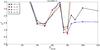 |
Fig. 4 Results of the HC3N modelling. The best reduced χ2 optimised with respect to Xin and Xout as a function of Tjump. |
The HC3N SLED has been analysed in two steps, as follows.
Step 1: we first ran a grid of models varying Tjump, Xin, and Xout with α = 0. The best fit for this first step was obtained with Tjump = 80 K, Xin = 3.6 × 10⁻¹⁰, and Xout = 6.0 × 10⁻¹¹. However, the fit is not very good (reduced χ2 = 1.7). We plotted for each line the predicted velocity-integrated flux emitted from a shell at a radius r (namely dF/ dr ∗ r) as a function of the radius, as shown in Fig. A.2. For the three lines with the lowest J (from J = 9 to 11) the predicted shell-flux increases with the radius and abruptly stops at the maximum radius of the envelope. This means that these three lines are very likely contaminated by the molecular cloud, which could explain the poor χ2. In the second modelling step, we therefore excluded these lines and repeated the modelling, as described below.
Results of the HC3N modelling.
Step 2: we ran a grid of models as in step 1 and found a better χ2 (0.8). We therefore extended the analysis by varying the α parameter between −1 and +2, together with the other three parameters Tjump, Xin, and Xout. The results are reported in Fig. 4 and Table 2. We note that in Table 2, we also report the values of the abundance of the envelope, XT20, at a radius equal to the angular size of the beam with the lowest frequencies, namely  in diameter. At this radius, which is 2.75 × 1016 cm (around 1800 AU), the envelope dust temperature is 20 K.
Figure 4 shows the χ2 obtained for each value of α, minimised with respect to Xin and Xout, as a function of Tjump. A χ2 lower than unity is obtained with Tjump equal to 80 K and α equal to 0 and 1 (Table 2). Figure 5 shows the abundance profiles of HC3N as predicted by the best-fit models. We note that the four models have the same Tjump (80 K), and the same Xin (9 × 10⁻¹⁰) and XT20 at 20 K (~1 × 10-11), within a factor 2. Therefore, the determination of Tjump, Xin, and Xout at 20 K is very robust and depends very little on the assumption of the HC3N abundance distribution.
Given the similarity of our results regardless of α, in the following we only consider the case of α = 0. Figure A.3 shows the χ2 contour plots as a function of the inner Xin and outer Xout with Tjump = 80 K. Figure A.4 reports the ratio of the observed over predicted line fluxes as a function of the upper level energy of the transition, to show the goodness of the best-fit model. Finally, Fig. A.5 shows the predicted shell-flux as a function of the radius for a sample of lines. As a final remark, we note that we also ran LTE models and obtained approximately the same results, within 20% for Xin and Xout and the same Tjump and α.
Results of the analysis.
4.2.2. HC5N
Because we now had fewer lines, we decided to assume that HC5N follows the spatial distribution of HC3N and ran a grid of models with α = 0, and T = 80 K and Xin and Xout as free parameters. The Xin − Xoutχ2 surface is shown in Fig. A.3 and the ratio between the observed and best-fit predicted intensities is shown in Fig. A.4. Table 3 summarises the best-fit values. We only obtained an upper limit to the Xin abundance, ≤8 × 10-11, while the Xout abundance is ~1 × 10-11. When compared to HC3N, the HC5N abundance is therefore more than ten times lower in the hot corino region, while it is the same in the outer cold envelope.
4.2.3. DC3N
Following the discussion on the HC3N line analysis, we did not consider the three DC3N lines with the lowest upper level energy, as they are likely contaminated by the molecular cloud.
For the remaining three lines, we adopted the same strategy as for HC5N for the SLED analysis, namely we adopted α = 0, and T = 80 K and varied Xin and Xout. The results are shown in Figs. A.3 and A.4, and summarised in Table 3. We obtained an upper limit of Xin ≤ 4 × 10-11, while Xout is ≤5 × 10-12. This implies a deuteration ratio of ≤5% and 50% in the hot corino and cold envelope, respectively.
4.2.4. Undetected species and final remarks on the observations
As mentioned earlier, we did not detect larger cyanopolyynes or 13C isotopologues. For the undetected species we derived the upper limits to the abundance by assuming that the non-detected emission arises in the hot corino (with a temperature of 80 K, diameter = 2″, N(H2) = 1.5 × 1023 cm-2, and line FWHM = 6 km s-1), and cold envelope (with a temperature of 20 K, a diameter = 30′′, N(H2) = 3.5 × 1022 cm-2, and line FWHM = 3 km s-1), respectively. The results are listed in Table 3.
From the HC5N and DC3N modelling, we conclude that the detected lines of both species are dominated by the emission from the cold outer envelope, as we only obtain upper limits to their abundance in the warm inner region. This conclusion is coherent with the line widths reported in Table 1. The HC3N lines (see also Fig. A.1) show a clear separation between the low-energy transitions, for which the FWHM is around 3 km s-1, and the high-energy transitions, for which the FWHM is around 6 km s-1 or higher. This difference strongly suggests that the two sets of lines probe different regions. As the low-energy lines correspond to Eup values lower than 80 K, a very natural explanation is that they are dominated by emission from the cold envelope, whereas the high-energy lines (Eup ≥ 110 K) are dominated by emission from the inner warm region. As the HC5N and DC3N lines have a FWHM of about 3 km s-1, it is not surprising that our modelling concludes that they are dominated by emission from the cold envelope.
5. Chemical origin of HC3N
As discussed in the Introduction, HC3N is an ubiquitous molecule in the ISM. There are several routes by which a high HC3N abundance may arise. Briefly, HC3N can form through the following neutral-neutral reactions (e.g. Wakelam et al. 2015): 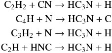 under typical dense-cloud conditions. Roughly, the first reaction contributes to about 80–90% of the formation of HC3N, with the other three swapping in importance depending on the initial conditions, but together contributing the remaining 20%. Its main destruction channels are either through reactions with He+ or reactions with atomic carbon, both contributing 30−40% to the destruction, depending on the initial conditions assumed. In dark clouds (nH~104−105 cm-3), it is well known that HC3N is abundant, together with other carbon chain molecules (e.g. Suzuki et al. 1992; Caselli et al. 1998). Thus, based on its routes of formation and destruction, we would expect the HC3N abundance to increase as a function of gas density, at least before freeze-out onto the dust grains takes over. Interestingly, however, the HC3N abundance with respect to H2 estimated in both the envelope and in the hot corino of IRAS 16293 is rather low (~10-11 and ~10-9, respectively). In this section we therefore discuss the possible physical conditions that may lead to such low abundances of HC3N.
5.1. Cold envelope
First of all, we investigated qualitatively which conditions in the cold envelope may lead to a fractional abundance of HC3N as low as 10-11. We would like to emphasise that this is difficult because very small changes in the main atomic elements (O, C, N) or molecular species (CO) can lead to very large changes in the abundances of tracers species. Hence, it is likely that small uncertainties in the initial elemental abundances of the cloud as well as its depletion history (which is dependent on the time the gas remains at a particular gas density) can easily lead to differences in the abundances of species such as HC3N of orders of magnitude.
For our analysis, we made use of the time-dependent chemical model UCL_CHEM (Viti et al. 2004). The code was used in its simplest form, namely we only included gas-phase chemistry with no dynamics (the gas was always kept at a constant density and temperature). The gas-phase chemical network is based on the UMIST database (McElroy et al. 2013) augmented with updates from the KIDA database as well as new rate coefficients for the HC3N and HC5N network as estimated by Loison et al. (2014). The chemical evolution was followed until chemical equilibrium was reached. To understand the chemical origin of the HC3N abundance that we measured in the cold envelope of IRAS 16293 (~10-11), we modelled a gas density of 2 × 106 cm-3 and a gas temperature of 20 K, which are the values inferred by Crimier et al. (2010) at a radius equivalent to the observations telescope beam (see Sect. 4.2.1).
We ran a small grid of models where we varied
the carbon and oxygen elemental abundances in the range of0.3–1 and 1–3 ×10⁻⁴, respectively;
the nitrogen elemental abundance: 6 (solar) and 2 × 10⁻⁵;
the cosmic-ray ionisation rate: 5 × 10-17 s-1 (assumed as our standard value) and 10 times higher.
We note that varying the C, O, and N elemental abundances can be considered approximately as mimicking qualitatively the degree of depletion of these elements onto the grain mantles. Furthermore, we varied the cosmic-ray ionisation rate because it is a rather uncertain parameter that could be enhanced with respect to the standard value because of the presence of X-rays or an energetic ≥ MeV particles source embedded inside the envelope (e.g. Doty et al. 2004; Ceccarelli et al. 2014b).
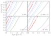 |
Fig. 6 Predicted HC3N abundance (in log) as a function of the O/H (x-axis) and C/H (y-axis) for four cases: the reference model, described in the text (upper left panel), and then the same, but with a cosmic-ray ionisation rate increased by a factor ten (upper right panel), a nitrogen elemental abundance decreased by a factor three (lower left panel) and at a time of 105 yr (lower right panel). The thick red lines mark the HC3N abundance measured in the cold envelope of IRAS 16293. |
The results of the modelling are plotted in Fig. 6. The top left panel is our reference model, with a standard cosmic-ray ionisation rate (5 × 10-17 s-1), at chemical equilibrium (≥106 yr), and with a solar abundance of nitrogen (6.2 × 10⁻⁵). The values of the HC3N abundances are log of the fractional abundance with respect to the total number of hydrogen nuclei, hence the best match with the observations is for a value of −11.3. We find that this value is reached within our reference model for low values of O/H (≤1.5 × 10⁻⁴) and for a O/C ratio between 1.5 and 2, with the lowest O/C ratio needed with the highest O/H abundance. This implies that both oxygen and carbon are mostly frozen onto the grain icy mantles by about the same factor, as the O/C ratio is similar to the one in the Sun (1.8; see e.g. Asplund et al. 2009) and in the HII regions (1.4; see e.g. García-Rojas & Esteban 2007). Increasing the cosmic-ray ionisation rate by a factor of ten changes the above conclusions little, having as an effect a slightly larger parameter space in O/H and O/C to reproduce the observed HC3N abundance. In contrast, decreasing N/H by a factor of three slightly diminishes the O/H and O/C parameter space. Finally, the largest O/H and O/C parameter space that reproduces the observed HC3N abundance in the cold envelope of IRAS 16293 is obtained by considering earlier times, 105 yr (bottom right of Fig. 6). This possibly implies that the gas in the envelope is at a similar age to that of the protostar.
5.2. Hot corino
As we move towards the centre of the protostar(s), a jump in the HC3N abundance by roughly two orders of magnitude is observed at around 80 K. This means that the first question to answer is what this 80 K represents. According to the temperature programmed desorption (TPD) experiments by Collings et al. (2004) and successive similar works, in general, the ice sublimation is a complex process and does not occur at one single temperature, but in several steps. In the particular case of iced HC3N, it is expected to have two sublimation peaks, at a dust temperature of about 80 and 100 K, respectively (for details, see Viti et al. 2004). The first corresponds to the so-called volcano ice desorption, and the second corresponds to the ice co-desorption, namely the whole ice sublimation. Therefore, our measured jump temperature of 80 K indicates that the most important sublimation is due to the volcano desorption, while the co-desorption injects back only a minor fraction of the frozen HC3N. In addition, the 80 K jump also tells us that any other processes contributing to the formation of HC3N at lower (≤80 K) temperatures have to be negligible. In other words, considering the reactions in the synthesis of HC3N reported at the beginning of Sect. 5, the desorption of C-bearing iced species, for example CH4, has to provide a negligible contribution to the HC3N abundance.
To understand what all this implies, we ran UCL_CHEM again, but this time we included freeze-out of the gas species in the cold phase to simulate the cold and dense prestellar phase. We then allowed thermal evaporation of the icy mantles as a function of the species and temperature of the dust following the recipe of Collings et al. (2004), in which the ice sublimation occurs in several steps (for details, see Viti et al. 2004). We find that the jump in the HC3N abundance from 10-11 to 10-9 occurs only if thermal evaporation due to the volcano peak occurs quickly, on a timescale of ≤103−4 yr, implying that the increase in the dust temperature to ~80 K must also occur quickly, on a similar timescale. In addition, if frozen species containing C, such as CO and CH4, sublimate at earlier times, namely at colder temperatures, and remain in the gas for too long before the volcano explosion, then the HC3N abundance reaches much too high abundances too quickly. In other words, the sublimation of these species must have occurred not much before the volcano sublimation, again on timescales of ≤103 yr.
5.3. HC5N
We finally note that none of our models can reproduce an HC5N abundance comparable to the one of HC3N, as observed in the cold envelope of IRAS 16293. All models predict a much lower HC5N abundance, by more than a factor ten, than the HC3N abundance. Since in the warm (T ≥ 80 K) region we only derive an upper limit for the HC5N abundance (which is at least ten times lower than that of HC3N), the models cannot be constrained. The failure of our models to reproduce HC5N in the cold envelope is most likely due to a lack of a comprehensive network for the formation and destruction of the species HC5N and therefore calls for a revision of its gaseous chemistry. Here we briefly summarize the main routes of formation and destruction for this species in our models: 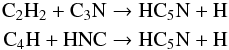 contributing to its formation by ~70% and 30%, respectively, and
 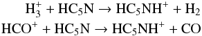 contributing to its destruction by ~50% and 40%, respectively.
It is clear that since both HC3N and HC5N are tracer species (with abundances ≤10-9), at least in this particular source, a more complete network is required, possibly including cyanopolynes with a higher number of carbon than included here, together with a proper treatment of the gas-grain chemistry that is needed to properly model the cold envelope. This will be the scope of future work.
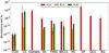 |
Fig. 7 Abundances of cyanopolynes in different sources: IRAS 16293 outer envelope (IT20) and inner region (Iin; this work), cold clouds (CC; Winstanley & Nejad 1996; Miettinen 2014), comet Hale-Bopp at 1 AU assuming H2O/H2 = 5 × 10⁻⁵ (Comets; Bockelé- Morvan et al. 2000), first hydrostatic core sources (FHSC; Cordiner et al. 2012), warm carbon-chain chemistry sources (WCCC; Sakai et al. 2008, 2004), massive hot cores (HC; Schöier et al. 2002; Esplugues et al. 2013), outflow sources (OF; Bachiller & Pérez Gutiérrez 1997; Schöier et al. 2002, Galactic Centre clouds (GCC; Marr et al. 1993; Aladro et al. 2011), and external galaxies (EG; Aladro et al. 2011). |
6. Discussion
6.1. General remarks on cyanopolyynes in different environments
In the Introduction, we mentioned that cyanopolyynes are almost ubiquitous in the ISM. Here we compare the cyanopolyyne abundance derived in this work with that found in various Galactic and extragalactic environments that possess different conditions (temperature, density, and history). Figure 7 graphically shows this comparison. From this figure, we note the following: (i) HC3N is present everywhere in the ISM with relatively high abundances; (ii) the abundance in the cold envelope of IRAS 16293 is the lowest in the plot, implying a high degree of freezing of oxygen and carbon, as indeed suggested by the chemical model analysis; (iii) HC3N and HC5N have relatively similar abundances in the IRAS 16293 outer envelope, cold cloud, first hydrostatic core (FHSC), and WCCC sources, namely in the cold objects of the figure, implying that the derived ratio HC5N/HC3N ~ 1 in the IRAS 16293 cold envelope is not, after all, a peculiarity, but probably due to the cold temperature; and finally; (iv) DC3N is only detected in cold objects except in the warm envelope of IRAS 16293 and the hot cores, suggesting that in these sources, it is linked to the mantle sublimation, in one way or another, as again found by our chemical modelling.
6.2. Present and past history of IRAS 16293
Our analysis of the TIMASSS spectral survey reveals the presence of HC3N, HC5N, and DC3N in IRAS 16293. HC3N was previously detected by van Dishoeck et al. (1993), and its abundance has been analysed by Schöier et al. (2002) with a two-step abundance model, where the jump was assumed to occur at 90 K. Schöier et al. (2002) found HC3N/H2 ~ 10-9 in the inner warm part and ≤~10-10 in the outer envelope. We note that they were unable to derive a value for the outer envelope or estimate where the jump occurs because they only detected three lines. Nonetheless, their estimates are in excellent agreement with our new estimates (Table 3).
A very important point is that we were not only able to estimate the cold envelope abundance, but also to determine where the jump occurs, an essential information for the determination of the origin of HC3N in IRAS 16293. Our chemical modeling (Sect. 5) showed that in the cold envelope, the HC3N abundance is reproduced for low values of oxygen and carbon in the gas phase, implying that these species are heavily frozen onto the grain mantles. The O/C ratio is between 1.5 and 2, similar to solar, if the chemistry of the envelope is a fossil, namely built up during the ~107 yr life of the parental molecular cloud. If, in contrast, the chemistry was reset (for any reason) and evolved in a shorter time, for instance in 105 yr, the O/C ratio that reproduces the observations could be as high as 3, but the oxygen and carbon have anyway remained mostly frozen onto the grain mantles. Probably the most important point to remark is that the HC3N abundance is very low, a very tiny fraction of the CO abundance, the main reservoir of the carbon, so that little variation in the CO abundance results in large variation in the HC3N abundance.
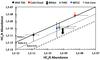 |
Fig. 8 Abundance of HC5N as a function of the abundance of HC3N in different protostellar and cold sources: inner (black arrow) and outer envelope (T20) of IRAS 16293 (black filled circle) presented in this work, warm carbon-chain chemistry (WCCC) sources (blue diamond; Sakai et al. 2008; Jørgensen et al. 2004), first hydrostatic core (FHSC) source (green triangle; Cordiner et al. 2012), hot cores sources (cross; Schöier et al. 2002; Esplugues et al. 2013), and Galactic Centre clouds (red square; Marr et al. 1993; Aladro et al. 2011). |
A second extremely interesting point is that the HC3N abundance undergoes a jump of about one hundred when the dust temperature reaches 80 K. These two values provide us with very strong constraints on how the collapse of IRAS 16293 occurred: it must have occurred so fast that the sublimation of C-bearing ices, such as CO and methane, has not yet produced HC3N in enough large abundances to mask the jump that is due to the volcano sublimation of the ices at 80 K (Collings et al. 2004; Viti et al. 2004). An approximate value of this time is ~103 yr, based on our modelling. In other words, the HC3N measured abundance jump temperature and abundance in the warm envelope both suggest that IRAS 16293 is a very young object, as expected, and that the envelope dust heating took no more than ~103 yr to occur.
A third result from the present study is the large measured abundance of HC5N, for the first time detected in a solar-type protostar. It is indeed only ten times lower than HC3N in the inner warm region and similar to the HC3N abundance in the outer cold envelope. When compared to other protostellar sources where HC5N has been detected, this ratio is not so anomalous. Figure 8 shows the two abundances in several protostellar sources and cold clouds. The two coldest sources have both an HC5N/HC3N ~ 1, while in the other sources this ratio is ~0.1. However, our chemical model fails to reproduce such a high abundance of HC5N, even though we included part of the most updated chemical network, recently revised by Loison et al. (2014). Evidently, we are missing key reactions that form this species.
6.3. HC3N deuteration
Finally, we detected for the first time the DC3N in a solar-type protostar. The deuteration of HC3N is about 50% in the outer cold envelope and lower than 5% in the warm part. This also provides us with important clues on the present and past history of IRAS 16293. First, the high deuteration in the cold envelope tells us that this is a present-day product, namely it is caused by a cold and CO-depleted gas, in agreement with previous observations and theoretical predictions (e.g. Ceccarelli et al. 2014a).
The very low deuteration in the warm part is, in contrast, more intriguing. It cannot be the result of an initial high deuteration that has been diminished by gas-phase reactions, because, as we have argued above, HC3N is the result of the volcano sublimation, which occurred because of a quick, ≤103 yr, heating of the dust. This means that it must be a fossil from the dust before the warming phase. This is probably one of the few very clear cases of fossil deuteration where there are no doubts that it is pristine (another one, to our knowledge, is the one of HDCO in the protostellar molecular shock L1157-B1; Fontani et al. 2014). The deuteration in IRAS 16293 is very high in general, with a doubly deuterated ratio of formaldehyde of ~30%, for example (Ceccarelli et al. 1998), and a triply deuterated ratio of methanol of a few percent (Parise et al. 2004). While at present we still do not have a clear measure of the formaldehyde deuteration in the warmer and colder envelope separately (e.g. Ceccarelli et al. 2001), methanol should be entirely concentrated in the warm region. However, recently, deuterated formamide (NH2CDO and NHDCHO) has been detected by ALMA in IRAS 16293, and the observations clearly show that formamide line emission is associated with the warm hot corino (Coutens et al. 2016). The measured deuteration ratio is a few percent, similar to that found in HC3N in the present work. Therefore, the molecular deuteration is a complex phenomenon even within the same source.
If our reasoning above is correct, namely the present-day gaseous HC3N is the sublimation product of previously frozen HC3N, then its relatively low deuteration tells us that this species is an early chemical product, namely it was formed in a time when the gas temperature was not too low and, mostly importantly, the CO was not depleted yet (see e.g. Ceccarelli et al. 2014a). This is in perfect agreement with the models of HC3N formation, which show that HC3N is abundantly formed before the full trapping of carbon into CO (see e.g. Loison et al. 2014, and Sect. 5). Therefore, the low DC3N/HC3N in the warm part is well explained by the picture that abundant HC3N has been formed during the tenuous molecular cloud phase and then frozen onto the ice mantles when the condensation that gave birth to IRAS 16293 increased in density while it decreased in temperature. Then, we predict that the deuteration of HC3N in the hot corino regions could be a good probe of the timescale of the collapse as well. Of course, detailed modelling will be necessary to quantify this prediction.
Meanwhile, the collection of previous measures of DC3N/HC3N, shown in Fig. 9, provides support to our thesis. With the exception of the cold envelope of IRAS 16293, all other sources where DC3N has been observed, possess a HC3N deuteration of a few percent, in agreement with the hypothesis that HC3N is an early chemical product.
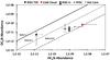 |
Fig. 9 Abundance of DC3N as a function of the abundance of HC3N in different protostellar and cold sources. The symbols are the same as those in Fig. 8. |
7. Conclusions
We detected several lines from cyanoacetylene (HC3N) and cyanodiacetylene (HC5N), and provided an upper limit to the abundance of cyanotriacetylene (HC7N) and other undetected cyanopolyynes. We also reported the first detection of deuterated cyanoacetylene, DC3N, in a solar-type protostar. In contrast, we did not detect any 13C cyanopolyyne isotopologue. We found that the HC3N abundance is roughly constant (~1.3 × 10⁻¹¹) in the outer cold envelope of IRAS 16293-2422 and it increases, as a step-function, by about a factor 100 in the inner region where the dust temperature exceeds 80 K. The HC5N has an abundance similar to HC3N in the outer envelope and about a factor of ten lower in the inner region.
A comparison with a chemical model provided constraints on the oxygen and carbon gaseous abundance in the outer envelope and, most importantly, on the age of the source. The HC3N abundance derived in the inner region and where the jump occurs also provided strong constraints on the time taken for the dust to warm up to 80 K, which has to be less than ~103−104 yr.
Finally, the cyanoacetylene deuteration is about 50% in the outer envelope and ~5% in the warm inner region. The relatively low deuteration in the warm region suggests that we are seeing an almost pristine fossil of the HC3N, abundantly formed in the tenuous phase of the pre-collapse and then frozen into the grain mantles at a later phase.
Acknowledgments
This research was supported in part by the National Science Foundation under Grant No. NSF PHY11-25915. We acknowledge the financial support from the university of Al-Muthana and ministry of higher education and scientific research in Iraq. E.M. acknowledges support from the Brazilian agency FAPESP under grants 2014/22095-6 and 2015/22254-0.
References
- Aladro, R., Martín-Pintado, J., Martín, S., Mauersberger, R., & Bayet, E. 2011, A&A, 525, A89 [NASA ADS] [CrossRef] [EDP Sciences] [Google Scholar]
- Asplund, M., Grevesse, N., Sauval, A. J., & Scott, P. 2009, ARA&A, 47, 481 [NASA ADS] [CrossRef] [Google Scholar]
- Bachiller, R., & Pérez Gutiérrez, M. 1997, ApJ, 487, L93 [NASA ADS] [CrossRef] [Google Scholar]
- Bell, M. B., Feldman, P. A., Travers, M. J., et al. 1997, ApJ, 483, L61 [NASA ADS] [CrossRef] [Google Scholar]
- Ben Abdallah, D., Najar, F., Jaidane, N., Dumouchel, F., & Lique, F. 2012, MNRAS, 419, 2441 [NASA ADS] [CrossRef] [Google Scholar]
- Bockelée-Morvan, D., Lis, D. C., Wink, J. E., et al. 2000, A&A, 353, 1101 [NASA ADS] [Google Scholar]
- Brack, A. 1998, in The Molecular Origins of Life: Assembling Pieces of the Puzzle (Cambridge University Press) [Google Scholar]
- Caselli, P., & Ceccarelli, C. 2012, A&ARv, 20, 56 [NASA ADS] [CrossRef] [MathSciNet] [Google Scholar]
- Caselli, P., Walmsley, C. M., Terzieva, R., & Herbst, E. 1998, ApJ, 499, 234 [NASA ADS] [CrossRef] [Google Scholar]
- Caux, E., Kahane, C., Castets, A., et al. 2011, A&A, 532, A23 [NASA ADS] [CrossRef] [EDP Sciences] [Google Scholar]
- Cazaux, S., Tielens, A. G. G. M., Ceccarelli, C., et al. 2003, ApJ, 593, L51 [NASA ADS] [CrossRef] [Google Scholar]
- Ceccarelli, C., Hollenbach, D. J., & Tielens, A. G. G. M. 1996, ApJ, 471, 400 [Google Scholar]
- Ceccarelli, C., Castets, A., Loinard, L., Caux, E., & Tielens, A. G. G. M. 1998, A&A, 338, L43 [NASA ADS] [Google Scholar]
- Ceccarelli, C., Castets, A., Caux, E., et al. 2000, A&A, 355, 1129 [NASA ADS] [Google Scholar]
- Ceccarelli, C., Loinard, L., Castets, A., et al. 2001, A&A, 372, 998 [NASA ADS] [CrossRef] [EDP Sciences] [Google Scholar]
- Ceccarelli, C., Maret, S., Tielens, A. G. G. M., Castets, A., & Caux, E. 2003, A&A, 410, 587 [NASA ADS] [CrossRef] [EDP Sciences] [Google Scholar]
- Ceccarelli, C., Caselli, P., Bockelée-Morvan, D., et al. 2014a, Protostars and Planets VI, 859 [Google Scholar]
- Ceccarelli, C., Dominik, C., López-Sepulcre, A., et al. 2014b, ApJ, 790, L1 [NASA ADS] [CrossRef] [Google Scholar]
- Chandler, C. J., Brogan, C. L., Shirley, Y. L., & Loinard, L. 2005, ApJ, 632, 371 [NASA ADS] [CrossRef] [Google Scholar]
- Clarke, D. W., & Ferris, J. P. 1995, Icarus, 115, 119 [NASA ADS] [CrossRef] [Google Scholar]
- Collings, M. P., Anderson, M. A., Chen, R., et al. 2004, MNRAS, 354, 1133 [NASA ADS] [CrossRef] [Google Scholar]
- Cordiner, M. A., Charnley, S. B., Wirström, E. S., & Smith, R. G. 2012, ApJ, 744, 131 [NASA ADS] [CrossRef] [Google Scholar]
- Coutens, A., Jørgensen, J. K., van der Wiel, M. H. D., et al. 2016, A&A, 590, L6 [Google Scholar]
- Crimier, N., Ceccarelli, C., Maret, S., et al. 2010, A&A, 519, A65 [NASA ADS] [CrossRef] [EDP Sciences] [Google Scholar]
- Doty, S. D., Schöier, F. L., & van Dishoeck, E. F. 2004, A&A, 418, 1021 [NASA ADS] [CrossRef] [EDP Sciences] [Google Scholar]
- Esplugues, G. B., Cernicharo, J., Viti, S., et al. 2013, A&A, 559, A51 [NASA ADS] [CrossRef] [EDP Sciences] [Google Scholar]
- Faure, A., Lique, F., & Wiesenfeld, L. 2016, MNRAS, 460, 2103 [NASA ADS] [CrossRef] [Google Scholar]
- Fontani, F., Codella, C., Ceccarelli, C., et al. 2014, ApJ, 788, L43 [NASA ADS] [CrossRef] [Google Scholar]
- Friesen, R. K., Medeiros, L., Schnee, S., et al. 2013, MNRAS, 436, 1513 [NASA ADS] [CrossRef] [Google Scholar]
- García-Rojas, J., & Esteban, C. 2007, ApJ, 670, 457 [NASA ADS] [CrossRef] [Google Scholar]
- Goesmann, F., Rosenbauer, H., Bredehöft, J. H., et al. 2015, Science, 349, 6247 [CrossRef] [Google Scholar]
- Jaber, A. A., Ceccarelli, C., Kahane, C., & Caux, E. 2014, ApJ, 791, 29 [Google Scholar]
- Jørgensen, J. K., Schöier, F. L., & van Dishoeck, E. F. 2004, A&A, 416, 603 [NASA ADS] [CrossRef] [EDP Sciences] [Google Scholar]
- Jørgensen, J. K., Bourke, T. L., Nguyen Luong, Q., & Takakuwa, S. 2011, A&A, 534, A100 [NASA ADS] [CrossRef] [EDP Sciences] [Google Scholar]
- Loinard, L., Torres, R. M., Mioduszewski, A. J., & Rodríguez, L. F. 2008, ApJ, 675, L29 [NASA ADS] [CrossRef] [Google Scholar]
- Loinard, L., Zapata, L. A., Rodríguez, L. F., et al. 2013, MNRAS, 430, L10 [NASA ADS] [CrossRef] [Google Scholar]
- Loison, J.-C., Wakelam, V., Hickson, K. M., Bergeat, A., & Mereau, R. 2014, MNRAS, 437, 930 [NASA ADS] [CrossRef] [Google Scholar]
- Loomis, R. A., Shingledecker, C. N., Langston, G., et al. 2016, MNRAS, 463, 4175 [NASA ADS] [CrossRef] [Google Scholar]
- Lunine. 2009, EPJ Web Conf., 1, 267 [CrossRef] [EDP Sciences] [Google Scholar]
- Marr, J. M., Wright, M. C. H., & Backer, D. C. 1993, ApJ, 411, 667 [NASA ADS] [CrossRef] [Google Scholar]
- McElroy, D., Walsh, C., Markwick, A. J., et al. 2013, A&A, 550, A36 [NASA ADS] [CrossRef] [EDP Sciences] [Google Scholar]
- Miettinen, O. 2014, A&A, 562, A3 [NASA ADS] [CrossRef] [EDP Sciences] [Google Scholar]
- Mizuno, A., Fukui, Y., Iwata, T., Nozawa, S., & Takano, T. 1990, ApJ, 356, 184 [NASA ADS] [CrossRef] [Google Scholar]
- Müller, H. S. P., Schlöder, F., Stutzki, J., & Winnewisser, G. 2005, J. Mol. Struct., 742, 215 [NASA ADS] [CrossRef] [Google Scholar]
- Mundy, L. G., Wootten, A., Wilking, B. A., Blake, G. A., & Sargent, A. I. 1992, ApJ, 385, 306 [NASA ADS] [CrossRef] [Google Scholar]
- Parise, B., Castets, A., Herbst, E., et al. 2004, A&A, 416, 159 [NASA ADS] [CrossRef] [EDP Sciences] [Google Scholar]
- Pickett, H. M., Poynter, R. L., Cohen, E. A., et al. 1998, J. Quant. Spectr. Rad. Transf., 60, 883 [NASA ADS] [CrossRef] [Google Scholar]
- Pineda, J. E., Maury, A. J., Fuller, G. A., et al. 2012, A&A, 544, L7 [NASA ADS] [CrossRef] [EDP Sciences] [Google Scholar]
- Sakai, N., Sakai, T., Hirota, T., & Yamamoto, S. 2008, ApJ, 672, 371 [NASA ADS] [CrossRef] [Google Scholar]
- Schöier, F. L., Jørgensen, J. K., van Dishoeck, E. F., & Blake, G. A. 2002, A&A, 390, 1001 [NASA ADS] [CrossRef] [EDP Sciences] [Google Scholar]
- Snell, R. L., Schloerb, F. P., Young, J. S., Hjalmarson, A., & Friberg, P. 1981, ApJ, 244, 45 [NASA ADS] [CrossRef] [Google Scholar]
- Suzuki, H., Yamamoto, S., Ohishi, M., et al. 1992, ApJ, 392, 551 [NASA ADS] [CrossRef] [Google Scholar]
- van Dishoeck, E. F., Blake, G. A., Draine, B. T., & Lunine, J. I. 1993, in Protostars and Planets III, eds. E. H. Levy, & J. I. Lunine, 163 [Google Scholar]
- Viti, S., Collings, M. P., Dever, J. W., McCoustra, M. R. S., & Williams, D. A. 2004, MNRAS, 354, 1141 [NASA ADS] [CrossRef] [Google Scholar]
- Wakelam, V., Loison, J.-C., Herbst, E., et al. 2015, ApJS, 217, 20 [NASA ADS] [CrossRef] [Google Scholar]
- Wernli, M., Wiesenfeld, L., Faure, A., & Valiron, P. 2007, A&A, 464, 1147 [NASA ADS] [CrossRef] [EDP Sciences] [Google Scholar]
- Winstanley, N., & Nejad, L. A. M. 1996, Ap&SS, 240, 13 [NASA ADS] [CrossRef] [Google Scholar]
- Wootten, A. 1989, ApJ, 337, 858 [NASA ADS] [CrossRef] [Google Scholar]
- Zapata, L. A., Loinard, L., Rodríguez, L. F., et al. 2013, ApJ, 764, L14 [NASA ADS] [CrossRef] [Google Scholar]
Appendix A: Figures that show the HC3N modelling
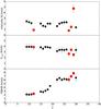 |
Fig. A.1 HC3N line intensity (upper panel), rest velocity VLSR (middle panel), and FWHM (bottom panel) as a function of the upper J of the transition. The red squares show the lines that have been discarded because they did not satisfy all criteria 3 to 5 of Sect. 3.2 (see text). |
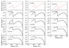 |
Fig. A.2 Predicted contribution to the integrated line intensity (dF/ dr ∗ r) of a shell at a radius r for the HC3N lines. This model corresponds to α = 0, Tjump = 80 K, Xin = 3.6 × 10⁻¹⁰, and Xout = 6.0 × 10⁻¹¹. The three upper red dashed curves show an increasing emission towards the maximum radius and very likely contaminated by the molecular cloud (see Sect. 4.2.1). |
 |
Fig. A.3 χ2 contour plots for HC3N (left), HC5N (middle) and DC3N (right) as a function of Xin and Xout. The predictions refer to a model with Tjump = 80 K and α = 0. |
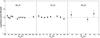 |
Fig. A.4 Ratio of the observed over predicted line flux as a function of the upper level energy of the transition for the model 2 (Tjump = 80 K and α = 0), for HC3N (left), HC5N (middle), and DC3N (right), respectively. |
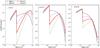 |
Fig. A.5 Velocity-integrated flux emitted from each shell at a radius r (dF/ dr ∗ r) as a function of the radius for the HC3N four best NLTE model, for three low, middle, and high values of J. |
All Tables
All Figures
|
Fig. 1 Observed spectra of the detected lines of HC3N. The red curves show the Gaussian fits. The temperature is a main-beam antenna temperature. |
| In the text | |
|
Fig. 2 Observed spectra of the detected lines of HC5N. The red curves show the Gaussian fits. The temperature is a main-beam antenna temperature. |
| In the text | |
|
Fig. 3 Observed spectra of the detected lines of DC3N. The red curves show the Gaussian fits. The temperature is a main-beam antenna temperature. |
| In the text | |
|
Fig. 4 Results of the HC3N modelling. The best reduced χ2 optimised with respect to Xin and Xout as a function of Tjump. |
| In the text | |
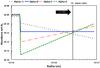 |
Fig. 5 Abundance profiles of the four HC3N best-fit models of Table 2. |
| In the text | |
|
Fig. 6 Predicted HC3N abundance (in log) as a function of the O/H (x-axis) and C/H (y-axis) for four cases: the reference model, described in the text (upper left panel), and then the same, but with a cosmic-ray ionisation rate increased by a factor ten (upper right panel), a nitrogen elemental abundance decreased by a factor three (lower left panel) and at a time of 105 yr (lower right panel). The thick red lines mark the HC3N abundance measured in the cold envelope of IRAS 16293. |
| In the text | |
|
Fig. 7 Abundances of cyanopolynes in different sources: IRAS 16293 outer envelope (IT20) and inner region (Iin; this work), cold clouds (CC; Winstanley & Nejad 1996; Miettinen 2014), comet Hale-Bopp at 1 AU assuming H2O/H2 = 5 × 10⁻⁵ (Comets; Bockelé- Morvan et al. 2000), first hydrostatic core sources (FHSC; Cordiner et al. 2012), warm carbon-chain chemistry sources (WCCC; Sakai et al. 2008, 2004), massive hot cores (HC; Schöier et al. 2002; Esplugues et al. 2013), outflow sources (OF; Bachiller & Pérez Gutiérrez 1997; Schöier et al. 2002, Galactic Centre clouds (GCC; Marr et al. 1993; Aladro et al. 2011), and external galaxies (EG; Aladro et al. 2011). |
| In the text | |
|
Fig. 8 Abundance of HC5N as a function of the abundance of HC3N in different protostellar and cold sources: inner (black arrow) and outer envelope (T20) of IRAS 16293 (black filled circle) presented in this work, warm carbon-chain chemistry (WCCC) sources (blue diamond; Sakai et al. 2008; Jørgensen et al. 2004), first hydrostatic core (FHSC) source (green triangle; Cordiner et al. 2012), hot cores sources (cross; Schöier et al. 2002; Esplugues et al. 2013), and Galactic Centre clouds (red square; Marr et al. 1993; Aladro et al. 2011). |
| In the text | |
|
Fig. 9 Abundance of DC3N as a function of the abundance of HC3N in different protostellar and cold sources. The symbols are the same as those in Fig. 8. |
| In the text | |
|
Fig. A.1 HC3N line intensity (upper panel), rest velocity VLSR (middle panel), and FWHM (bottom panel) as a function of the upper J of the transition. The red squares show the lines that have been discarded because they did not satisfy all criteria 3 to 5 of Sect. 3.2 (see text). |
| In the text | |
|
Fig. A.2 Predicted contribution to the integrated line intensity (dF/ dr ∗ r) of a shell at a radius r for the HC3N lines. This model corresponds to α = 0, Tjump = 80 K, Xin = 3.6 × 10⁻¹⁰, and Xout = 6.0 × 10⁻¹¹. The three upper red dashed curves show an increasing emission towards the maximum radius and very likely contaminated by the molecular cloud (see Sect. 4.2.1). |
| In the text | |
|
Fig. A.3 χ2 contour plots for HC3N (left), HC5N (middle) and DC3N (right) as a function of Xin and Xout. The predictions refer to a model with Tjump = 80 K and α = 0. |
| In the text | |
|
Fig. A.4 Ratio of the observed over predicted line flux as a function of the upper level energy of the transition for the model 2 (Tjump = 80 K and α = 0), for HC3N (left), HC5N (middle), and DC3N (right), respectively. |
| In the text | |
|
Fig. A.5 Velocity-integrated flux emitted from each shell at a radius r (dF/ dr ∗ r) as a function of the radius for the HC3N four best NLTE model, for three low, middle, and high values of J. |
| In the text | |
Current usage metrics show cumulative count of Article Views (full-text article views including HTML views, PDF and ePub downloads, according to the available data) and Abstracts Views on Vision4Press platform.
Data correspond to usage on the plateform after 2015. The current usage metrics is available 48-96 hours after online publication and is updated daily on week days.
Initial download of the metrics may take a while.