| Issue |
A&A
Volume 597, January 2017
|
|
|---|---|---|
| Article Number | A55 | |
| Number of page(s) | 13 | |
| Section | Stellar structure and evolution | |
| DOI | https://doi.org/10.1051/0004-6361/201629150 | |
| Published online | 21 December 2016 | |
CoRoT photometry and STELLA spectroscopy of an eccentric, eclipsing, and spotted HgMn binary with sub-synchronized rotation⋆,⋆⋆
Leibniz-Institute for Astrophysics Potsdam (AIP), An der Sternwarte 16, 14482 Potsdam, Germany
e-mail: This email address is being protected from spambots. You need JavaScript enabled to view it.
; This email address is being protected from spambots. You need JavaScript enabled to view it.
; This email address is being protected from spambots. You need JavaScript enabled to view it.
; This email address is being protected from spambots. You need JavaScript enabled to view it.
; This email address is being protected from spambots. You need JavaScript enabled to view it.
Received: 20 June 2016
Accepted: 7 October 2016
Abstract
Context. We report the discovery and analysis of very narrow transits in the eccentric spectroscopic binary HSS 348 (IC 4756).
Aims. The aim is to characterize the full HSS 348 system.
Methods. We obtained high-precision CoRoT photometry over two long runs and multi-epoch high-resolution échelle spectroscopy and imaging with STELLA. Standard radial-velocity extraction, spectrum synthesis, Fourier analysis, and light-curve inversions are applied to the data.
Results. HSS 348 is found to be an eccentric (e = 0.18) double-lined spectroscopic binary with a period of 12.47 d in which at least the primary component is a peculiar B star of the HgMn class. The orbital elements are such that the system undergoes a grazing eclipse with the primary in front but no secondary eclipse. The out-of-eclipse light variations show four nearly equidistant but unequal minima stable in shape and amplitude throughout our observations. Their individual photometric periods are all harmonics of the same fundamental period which happens to agree with the transit period to within the errors. We interpret the fundamental period to be the rotation period of at least one if not both stars due to surface inhomogeneities. Due to the non-zero eccentricity of the orbit the two components are rotating sub-synchronously.
Conclusions. It appears that HSS 348 is not a member of the IC 4756 cluster but a background B8+B8.5 binary system. Its sharp eclipses every 12.47 days just mimic a small-body transit but are in reality the grazing eclipses of a B-star binary and thus a classical false positive. The system seems to be pre-main sequence with the primary possibly just arrived on the ZAMS. The light curve with four unequal minima can be explained with four cool spots of different size equidistantly positioned in longitude. Our data do not allow to uniquely assign the spots to either of the two stars.
Key words: binaries: eclipsing / stars: chemically peculiar / stars: rotation / starspots / stars: individual: TYC 455-791-1 / open clusters and associations: individual: IC 4756
The CoRoT space mission, launched on 2006 December 27, has been developed and is operated by CNES, with the contribution of Austria, Belgium, Brazil, ESA (RSSD and Science Programme), Germany and Spain. Partly based on data obtained with the STELLA robotic observatory in Tenerife, an AIP facility jointly operated by AIP and IAC.
The final data sets are only available at the CDS via anonymous ftp to cdsarc.u-strasbg.fr (130.79.128.5) or via http://cdsarc.u-strasbg.fr/viz-bin/qcat?J/A+A/597/A55
© ESO, 2016
1. Introduction
Photometric transit detections from space are now made for many types of targets, in particular for exoplanets from CoRoT and Kepler and the future missions TESS and PLATO. In the course of our CoRoT program on the open cluster IC 4756, we detected a series of well-defined transits in one of our targets. The star is CoRoT 105328054, identified as HSS 348 in Herzog et al. (1975) and as TYC 455-791-1 in Høg et al. (2000). Its USNO-B1.0 number is USNO-B1.0 0950-0378805 and the J2000.0 coordinates are 18:39:44.30 and +05:01:22.8 (Zacharias et al. 2005) with corrected proper motions of −3.5 mas/yr in RA and −2.2 mas/yr in Dec (Roeser et al. 2010). The B and V magnitudes from the Tycho catalog (Høg et al. 2000) are 12 74 and 1195, respectively, and thus
  . Errors for this brightness range are expected to be 010. Herzog et al. (1975) only listed a B magnitude of 1281, while NOMAD (Zacharias et al. 2005) lists magnitudes in BVR of 12716, 11959 and 1147, respectively. Based on its brightness and proper motions, Herzog et al. (1975) assigned a 94% probability that it is an IC 4756 cluster member, which was incorrectly confirmed only recently by Strassmeier et al. (2015a, Paper I) on the basis of Strömgren photometry and a few radial velocities (RV). As we show in the present paper, the target is an eccentric double-lined spectroscopic binary and the RV subset previously available only accidentally mimicked the average cluster velocity.
Transiting targets can be considered as laboratories that allow the determination of parameters otherwise not easily accessible. For example, Johnson et al. (2011) found a brown dwarf from transits in Kepler light curves and determined its radius to 0.83 Jupiter radii with a precision of ≈4%. Masses and radii for five transiting M-dwarf stars in front of their F-type primaries from the TrES survey were determined by Fernandez et al. (2009). The authors derived average densities for these targets and verified that the M-dwarf radii were indeed larger than predicted by models. Another science avenue spans to the stability of multiple stellar systems because at one point we suspected our target to be a close quintuple system from the four-minima CoRoT light curve additional to the transit. There are several examples of photometric and spectroscopic quadruple systems in the literature, such as the double eclipsing binary CzeV343 (Caga & Pejcha 2012) or the SB-4 eclipsing system KIC424779 (Lehmann et al. 2012); and probably several more targets from the ASAS and OGLE surveys (e.g., Helminiak et al. 2015; Graczyk et al. 2011; Pawlak et al. 2013).
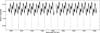 |
Fig. 1 CoRoT light curve of HSS 348. The time coverage is 173 consecutive days. Thirteen transits were covered. Note the periodic stellar light variations with four unequally deep minima but commensurable period. The brightness zero point is set arbitrarily to the Tycho V-band magnitude. |
An increasing number of eclipsing binaries with pulsating components also appear in the literature. A prominent example is even known in the open cluster IC 4756 (HD 172189, e.g., Ibanoglu et al. 2009). Age and close-binary evolution can also produce apparently exotic parameter combinations; Pietrzynski et al. (2012), for instance, identified RR-Lyrae-type pulsation with a period of 0.6 d in a 0.26 solar-mass star in a binary system, a combination that nature normally does not foresee. Tidally forced pulsations were long suspected in β-Cephei stars and slowly pulsating B stars (SPB; e.g., Aerts et al. 1998; Harmanec et al. 1997) and were recently confirmed from high-quality space photometry (e.g., for HD 174884 by Maceroni et al. 2009). Another group of late-B stars are the chemically peculiar HgMn stars (Hubrig & Mathys 1995). These stars are rotationally variables as a results of their inhomogeneous chemical surface abundances and/or local magnetic fields. Most of the HgMn stars are in spectroscopic binaries and about half of them are members of double-lined (SB2) systems with periods between 3–25 d (cf. Hubrig & Mathys 1995). A recent analysis by Balona (2016) verified that the number of rotational variables among B stars in the Kepler field is as high as among the A stars (about 40 per cent) with starspots as the likely cause of the photometric variability, although these targets do not have a significant convective envelope.
Our target was not detected in the ROSAT HRI survey by Randich et al. (1998). This constrains its X-ray luminosity to lower than ≈2 × 1029 erg s-1, even lower than what has been detected in the Hyades. With an age of 890 Myr (Strassmeier et al. 2015a) IC 4756 is nearly coeval with the Hyades where magnetic activity is already weak. In general, we therefore do not expect to see coronal activity on HSS 348. However, our target may still be interesting for understanding the evolutionary aspects of multiple stellar systems.
In the following, we present CoRoT time-series photometry of HSS 348 for two consecutive long runs, follow-up ground-based Strömgren photometry, and high-resolution spectra to determine radial velocities and other fundamental stellar parameters of this interesting target. Section 2 describes the data. Sections 3 and 4 analyze specifics of the light curves and the spectra, respectively, and Sect. 5 attempts to identify the astrophysical parameters of the system. Section 6 is our summary.
2. Observations
2.1. CoRoT photometry
CoRoT observed parts of IC 4756 from 2010 April 8 to September 24 (LRc05 and LRc06), that is, over a time span of 173 days. Data were delivered in form of two data sets broken up on HJD 2 455 385 by 88 h. We note for comparison that the satellite orbital period is 103 min. For the analysis, only the white-flux data have been used. Pure visual inspection reveals that most of the data points taken at passage of the South Atlantic Anomaly (SAA) had to be rejected. Furthermore, most of the outliers lie above the expected range and are mostly due to hot pixels and/or cosmic ray hits. Rejecting these obviously incorrect data points was a multi-step procedure, where each step involved smoothing the data set, then discarding all data points outside 3σ of the smoothed curve. The filtering could be understood as a Savitsky-Golay smoothing (SGS) on non-uniformly spaced data sets (e.g., Gerry 1991). As most of the invalid data are clustered around the SAA, classical SGS is not applicable further than the iteration progresses. For both data runs, we chose a half-width of the smoothing window of 0.1 days, which translates into a maximum number of 540 points at the original sampling of 32 s within the smoothing window. The fitting polynomial was chosen at order ten. The whole scheme stabilized after ten iterations, narrowing the data sets from originally 234 144 to 217 979, and from 208 193 to 193 798 data points for the first and second set, respectively. On the final data set, we checked the distribution of the residuals with respect to the smoothed set. A Gaussian distribution is not expected because most of the outliers are positive offsets, so that the Jarque-Bera test (Jarque & Bera 1987) still fails with a value of 287.4 and 240.1 for the first and second set, respectively, but was reduced from an original value of 1.1 × 10⁶ within the first iteration. From a quartile-to-quartile plot, no deviations from normally distributed residuals are seen. Furthermore, a fit of the histogram of the residuals to a Gaussian showed a correlation coefficient of 0.9985, giving us confidence that the cleaning procedure worked correctly. Finally, we used the residuals to estimate an average measurement error of 986 photoelectrons (e−) for the first data set and 1038 e− for the second data set. This is just ≈15% larger than the expected pure photon noise of 845 e−. For more details of the CoRoT data reduction process, we refer to Weingrill (2015). Contaminating stellar sources are identified and discussed in Sect. 3.1.
Even after rejecting outliers, zero-point jumps as reported by many other groups (e.g., Carone et al. 2012, and references therein) are still present in the data. We again used the smoothing polynomial but now its first, second and third derivative to detect regions of unexpected data jumps. Five such jumps were detected in total, four of them in the second data set. Owing to the high intrinsic variability of the star, no efforts to redeem these data points were made; we removed the affected points from the data. The final data sets then comprised 216 989 and 188 944 data points, respectively, and is available in electronic form at CDS Strasbourg. Figure 1 is a plot of these data converted and shifted to an average relative magnitude of 1195.
2.2. Follow-up spectroscopy
High-resolution spectra were obtained with the STELLA Echelle Spectrograph (SES) at the robotic 1.2-m STELLA-II telescope in Tenerife, Spain (Strassmeier et al. 2004, 2010). The SES is a fiber-fed white-pupil échelle spectrograph with a fixed wavelength format of 388–882 nm. The instrument is located in a separated room on a stabilized optical bench and is fed by a 12 m long 50 μm Ceram-Optec fiber (until August 2014). This fiber enabled a two-pixel resolution of R = 55 000. As of 2014/15, a 67 μm fibre and a two-slice image slicer replaced the smaller fibre that now enables a resolution of R = 65 000 and an entrance aperture of 2.0′′ on the sky. The CCD was an e2v 42-40 2048 × 2048 device until mid-2012, when it was replaced with an e2v 4k×4k 15 μm-pixel CCD. The guider images show the brightest CoRoT contaminating target (see Sect. 3.1) well separated from the pinhole at a distance of approximately 7.3′′.
Observations started in August 2012 and lasted until the end of 2015. Integrations were set to an exposure time of 120 min and achieved signal-to-noise ratios (S/N) between 20–50:1 per pixel depending on weather. A total of 39 spectra achieved S/N above 30:1; these were then used for analysis. This S/N is sufficient to obtain a radial-velocity precision of around 1 km s-1 for slowly rotating stars (see Strassmeier et al. 2012). The individual radial velocities are listed in the appendix (Table A.1). A typical sample spectrum is also shown in the appendix (Fig. C.1). SES spectra are automatically reduced and extracted using the IRAF-based STELLA data-reduction pipeline. For details we refer to Weber et al. (2008).
One spectrum of HSS 348 was taken with the 2 × 8.4 m Large Binocular Telescope (LBT) during commissioning of the PEPSI spectrograph (Potsdam Echelle Polarimetric and Spectroscopic Instrument; Strassmeier et al. 2015b). On May 26, 2015, PEPSI was used in its low-resolution mode with R = 43 000. Integration time was set to 20 min and S/N is 110:1 near Hα and 70:1 near Hβ. The observations were made with cross dispersers III and V and covered the wavelength ranges 478–542 nm and 620–742 nm, respectively.
2.3. Follow-up STELLA/WiFSIP photometry
Follow-up CCD photometry was obtained with the Wide Field STELLA Imaging Photometer (WiFSIP) at the second robotic 1.2-m telescope (STELLA-I) during the months May, June, and July 2011. Its CCD is a four-amplifier 4096 × 4096 15 μm pixel back-illuminated CCD from STA and was thinned and anti-reflection coated at the University of Arizona’s Imaging Technology Lab. The field of view with a three-lens field corrector is an unvignetted 22′×22′ with a scale of 0.32′′/pixel. The photometer is equipped with 90 mm sets of filters.
For HSS 348, we employed mostly Strömgren-uvby, and narrow (n) and wide (w) Hα and Hβ filters. Integrations were set to 91 s, 29 s, 28 s, 20 s, 160 s, 36 s, 160 s, and 36 s for uvby, Hβn, Hβw, Hαn, and Hαw. respectively. A nightly block consisted of five consecutive series of these eight filters with a total integration time of 2800 s. During three nights, two such consecutive blocks were executed. A total of nine images were also taken in Johnson BVR. An overview of the data log is given in the appendix. Only after data reduction did we notice that our Hβ filter had deteriorated such that it gave erroneous results. Therefore, we had to discard the new Hβ data.
The Johnson and the remaining Strömgren data were reduced in the same way as in Paper I. However, the zero point is now linked to the Tycho zero point (Høg et al. 2000) instead of to the eight stars in common with Hauck & Mermilliod (1998). Typically 20 observing sequences yielded the following grand average values for HSS 348: b−y = −0.04 ± 0.02, u−v = 0.33 ± 0.02, β = 2.727, c1 = 0.596, and (b−y)0 = −0.11 ± 0.02, m0 = −0.205, c0 = 0.58, with E(b−y) = 0.071. We note that the data quality from a single CCD frame is approximately 1% and thus not sufficient for time-series modulation work given the low amplitude of the target.
3. CoRoT light curves
3.1. Contamination
CoRoT contamination targets.
The unbinned light curve of HSS 348 is shown in Fig. 1. Target contamination for HSS 348 = CoRoT ID 105328054 has been predetermined in the Exo-Dat catalog (Deleuil et al. 2009) to just 1.2%, typically a negligible amount. However, digital sky images and our STELLA SES guider images showed at least one brighter target 7.3′′ away from HSS 348 (dubbed source A). A similar situation was encountered and analyzed by Paparó et al. (2011) for CoRoT 102781750, therefore we followed up the HSS 348 field with STELLA WiFSIP CCD imaging with higher pixel sampling and deeper exposures. It revealed three possible contaminating sources (A, B, and C, Fig. 2) within and at the rim of the CoRoT point-spread function (PSF) with a total contaminating flux of up to 4.1%. Table 1 gives the coordinates and magnitudes of these targets. Nine images were taken in Johnson V and stacked with SWarp (Bertin et al. 2002) to reach a limiting magnitude of ≈21 mag. The large aperture mask tailored to the PSF of CoRoT (for our observations 30″ × 18″) with its larger axis approximately in the N-S direction is also shown in Fig. 2. It does not fully encircle source A and we may assume only half of its flux for the contamination which would reduce the total contamination to 2.4%.
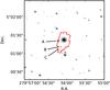 |
Fig. 2 CoRoT PSF footprint overlaid on a stacked STELLA WiFSIP CCD image. The CCD image is obtained with the Johnson V filter and has a limiting magnitude of 21 |
3.2. Detrending the data
We split the data into 500 phase bins, each comprising all data points of similar phases (phases are computed with respect to the eclipses). In each bin, we fit a fourth-order Legendre polynomial to all data points and kept the constant term as the data offset relevant for the bin in question. In the last step, we fit a fourth-order polynomial to all data points of all bins, now corrected for their phase-offsets determined in the previous step. The non-constant terms of this polynomial were then used to detrend the data. Care must be taken in the first step to use orthogonal polynomials, otherwise the determination of the constant offset is spoiled. One could either construct orthogonal polynomials from the data itself as described in Bevington (1967), for instance, or use Legendre polynomials, which are orthogonal in the range –1 to +1 in continuously sampled data.
Transit parameters for HSS 348.
3.3. Eclipse analysis
We first modeled the eclipses in the CoRoT light curve with the publicly available software JKTEBOP1 (Southworth et al. 2004, 2005, in version 34). It models the two components of a stellar binary as spheres for the eclipse shapes and is also frequently used for the light-curve modeling of transiting planets (e.g., Southworth et al. 2015; Mallonn et al. 2015). The fitting parameters are the sum of the fractional stellar radii, r1 + r2, and their ratio k = r2/r1, the orbital inclination i, the eclipse mid time T0 and the orbital period P. The index “1” refers to the primary component and “2” refers to the secondary component of the binary. The dimensionless fractional radius is the absolute radius in units of the orbital semi-major axis a, r1 = R1/a and r2 = R2/a. The stellar limb-darkening of the primary was included in the light-curve model by the quadratic limb-darkening law with the limb-darkening coefficients u and v. Both coefficients were fixed to theoretical values taken from Sing (2010) using the stellar parameters from Table 6. The eccentricity of the binary system and the argument of periastron were fixed to the values of Table 5 derived from the orbit solution in Sect. 4.2. The light-curve fit concentrated on the eclipse events, therefore we cut the data points farther away than 0.3 days from the eclipse center. In the case of detached eclipsing binaries consisting of two similar stars that undergo partial eclipses, the ratio of the radii k is poorly constrained by the light curves (e.g., Southworth et al. 2007). However, JKTEBOP allows the inclusion of the spectroscopic light ratio as an observational parameter into the light-curve fit. In Sect. 4.1, the spectroscopic light ratio was derived to be close to unity. After an initial fit, we employed the point-to-point scatter of the light curve residuals as photometric error bars. Additionally, we calculated the β factor per eclipse (Winn et al. 2008). The β factor describes the progression of the standard deviation σres of the time-binned light-curve residuals in comparison to σPoi of time-binned pure Poisson noise. In the presence of correlated noise in the photometric time series, σres is larger by the factor β than σPoi. We binned the residuals in intervals from 10 to 40 min in 2-min steps, derived the β value in each case, and finally used their average to inflate the photometric error bars. The mean β factor of the 13 individual eclipses is 1.39. The uncertainties of the eclipse parameters were estimated using a Monte Carlo simulation provided by JKTEBOP with 3000 iterations. The results of the final fit are given in Table 2 and are shown in Fig. 3.
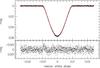 |
Fig. 3 Thirteen eclipse events phase folded and binned in 30 s intervals, and overplotted with the best-fit model (line). In the lower panel the residuals are shown with an rms of 0.47 mmag. We note that in this plot the orbital phase is centered on the mid-time of the eclipse. |
3.4. Out-of-eclipse period analysis
The CoRoT light curve in Fig. 1 is apparently dominated by at least three period components in an almost perfectly harmonic ratio to the eclipse/transit period of approximately 12.47 d (f ≈ 0.080 d-1). We first cut out the parts of the light curve that are apparently influenced by the transit. Then, Period04 (Lenz & Breger 2004) was used to calculate a discrete Fourier transformation from the remaining data. In both CoRoT data sets, eight harmonics at f, 2f, 3f, 4f, 6f, 8f, 10f, and 12f were identified. The moon introduced a ninth component at Pmoon = 29.424 ± 0.077 d in the first data set, and two components at Pmoon,1 = 30.27 ± 0.10 d and Pmoon,2 = 66.37 ± 0.34 d in the second data set. This model was then removed from the underlying variation and used to renormalize the two data blocks to a common data set, from which we modeled the transit in the previous section.
In a second step, the residuals from the transit removal were used to fill the transit gaps in the normalized light curve. After again subtracting the components introduced by the moon, and after merging and normalizing the two CoRoT observing epochs, a multi-frequency model yi was fit according to 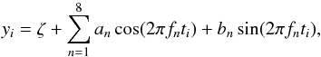 (1)with ζ,fn,an, and bn as free parameters. The ti are the times of measurements with a total of 405 929 data points. For a robust estimate of the parameter uncertainties, a Monte Carlo (MC) simulation was performed using 1000 random data sets. For each random data set, the times were kept fixed while the observed flux was allowed to vary normally distributed around the observed value assuming an error proportional to the photon noise but increased to match the rms of the original light-curve fit (1.59 mmag).
As a curiosity, the 12.46539 ± 0.00048-d period from the harmonic fit differed slightly but significantly from the transit period of 12.473707 ± 0.000012 d but was equal to within 1σ = 0.000023 d when the two data sets were treated independently (but otherwise using the same procedure). This was suspicious for hot stars, but might be explained for cool stars by a real change due to differential surface rotation. Normal hot stars do not exhibit surface differential rotation because of the lack of a (significant) convective envelope. Therefore, we also tested whether we could fit the light curve by forcing all the overtones to be integer multiples of a single fundamental frequency. This indeed recovered the fundamental and the transit period very accurately to nearly the same value of P0 = 12.473490 ± 0.000067 d with the same rms of 1.59 mmag with respect to the harmonic fit. We therefore believe that the orbital and the photometric periods could be identical but at least are within 3σ with respect to the out-of-eclipse period error. The peak-to-valley amplitudes of the eight strongest overtones are listed in Table 3 together with their errors which again were derived from a 1000 MC set. A phase-folded light curve with the fundamental period from the Fourier series together with the model light-curve is shown in Fig. 4.
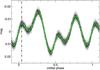 |
Fig. 4 Out-of-transit light curve folded with the fundamental period of P0 = 12.473490 ± 0.000067 d recovered from a twelve-component Fourier-series fit (line). Only every fourth data point is plotted. Eclipse points are removed. Orbital phase is according to the elements in Table 5. We note that periastron at the eclipse mid-time takes place at 0 |

Eight strongest overtones recovered with a fundamental period P0 = 12.4734940 ± 0.000067 d.
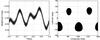 |
Fig. 5 Four-spot light-curve fit. Left: phased CoRoT light curve (the white line is the SML fit and the small dots are the CoRoT data from Fig. 1). Right: spot model in Mercator representation (from left to right identified as spots 1, 2, 3, and 4, see Table 4). We note that the phases of the four light-curve minima do not coincide with the central longitudes of the four spots but that the recovered spot longitudes agree with a time of periastron passage at phase 0 |
3.5. Rotational modulations due to starspots?
A double-humped light curve with Porb/ 2 is required by an ellipticity effect while a single-humped light cure with Porb is required by the reflection effect, following simple geometry. The light curve of HSS 348 is quadruple humped with two equidistant minima each at Porb/ 2. Such a light curve would require the second star to be geometrically distorted with a 90° phase shift with respect to the second component (the two larger stellar axes being perpendicular to each other). Moreover, our two stars are well separated and thus unlikely to be elliptical in shape, which would be required to generate a 30 mmag amplitude. Therefore, we exclude an ellipticity or a reflection effect as the sole cause for the photometric 12.47 d period.
Simple antipodal Ap-star spots on a rotating star would also produce a double-humped light curve. Two nearly equally bright stars with two spots on each of them could then, in principle, produce the observed quadruple-humped light curve if the antipodal spots are shifted on one component in longitude by 90° with respect to the spot locations on the other component. Another explanation is to place four equidistant spots on only one of the two stars, for example, the HgMn primary in our case. Unfortunately, the S/N ratio of our STELLA spectra does not allow to conclusively detect line-profile deformations that would have allowed us a spot assignment. We also note that with two (almost) equal stars it does not matter for the light-curve fit on which star we place the spots. Figure 5 is a phased time-series fit with our light-curve spot-modeling code SML (Ribarik et al. 2003). The program determines the position and size, (and temperature contrast) of spots by minimizing the fit residuals with the help of the Marquardt-Levenberg nonlinear least-squares algorithm. We allowed four circular spots on the HgMn primary and assumed equal intensity contrast proportional to an arbitrary temperature difference of 1000 K below the effective temperature (a value assumed from spotted cool stars, see Strassmeier 2009). A relative unspotted magnitude of –014 and a linear limb-darkening coefficient of 0.43 were adopted. The different light-curve minima were then modeled by adjusting the spot sizes and positions until the observed-minus-computed residuals approached the measurement uncertainties. The standard deviation for the fit in Fig. 5 is 0.51 mmag. We emphasize that these models bear only a minimal physical meaning and are mostly intended to show the geometric feasibility of a rotational-modulation explanation. A circular shape for the spots is only the simplest assumption and is most likely unrealistic. We also note that spot solutions from light curves are mathematically not unique because, first, light curves are one-dimensional data and maps are two dimensional, second, we cannot distinguish between the two hemispheres due to the equator-on view and, thirdly, we can not uniquely assign the spots to one of the two stellar components.
Circular spot model.
Because the light-curve shape of HSS 348 remained constant within the duration of our observations, its spots must have been as well. This is indeed expected if the spots are due to a mix of chemical inhomogeneities and suppressed convection of what is left of convection on a 13 000 K warm surface. Such a stable spot configuration, in size and in the position required by our CoRoT light curve, might be achieved by gravitational coupling with a multi-pole (inter-binary?) magnetic field. We emphasize that the comparably large amplitude of HSS 348 of up to 30 mmag cannot be solely due to chemical inhomogeneity because there are not enough spectral lines for such a strong blanketing effect (see our spectrum in Fig. 6). In several recent papers, Balona (2013, 2016) invoked atmospheric inhomogeneities such as magnetic starspots and/or “some other co-rotating structure” to explain the Kepler and K2 B- and A-star modulations even though there is no significant convective envelope. At this point we also re-emphasize that a Zeeman-Doppler image of the massive B0-star τ Sco (Donati et al. 2006) revealed a complex magnetic field distribution very comparable to that of the solar corona.
3.6. Pulsations?
The four light-curve minima are, in principle, also explainable by non-radial pulsations on only one stellar component but with four surface nodes or, alternatively, with two phase-locked nodes but from both stars. Tidal interaction may then synchronize the pulsation to the orbital motion. However, such long-period pulsations were not seen in this complexity so far (see, e.g., Aerts et al. 1998). Although we cannot explicitly exclude this scenario it appears less likely to us than the rotational hypothesis in the previous section.
4. Spectrum analysis
4.1. Identification of spectral features
Profiles from Balmer Hα (Fig. 6a), Hβ, and Hγ appear double-lined, each with a narrow line core and broad wings, typical for hot stars. Their disentangled equivalent widths (EW) from our R = 43 000 PEPSI spectrum are identical for the two components to within the measuring errors; 5.7 Å, and 5.1 Å for Hα and Hβ, respectively. To first order, we assume zero brightness difference between the two visible components at these wavelengths. However, a Balmer decrement Hα/Hβ of greater than unity is unexpected for normal mid-to-late B stars (e.g., Collins et al. 1991).
A number of singly ionized lines are detected that appear doubled and well separated by up to ≈160 km s-1 (Fig. 6b). Among the strongest are Si ii λ6347, 6371, 5978, 5056, 5041, Mg ii 4481, Fe ii 5316, 5019, 4924, 4731, and one (weaker) Ti/Cr ii blend at 4549 Å. Six pairs of relatively unblended lines were measured for line broadening by fitting a Gaussian profile to each of them. The average EW ratio is 0.76 ± 0.04 (primary/secondary), while the line-depth ratio at λ6350 Å, for example, is 1.40 ± 0.04 (primary/secondary), the error being the rms of the line intensities measured. The lowest values for the (instrumentally deconvolved) FWHM in Å at red wavelengths for the primary and secondary is 0.22 ± 0.02 and 0.47 ± 0.05, respectively. These are converted into vsini’s with the calibration of Fekel (1997) and return values of 10 and 25 km s-1, respectively. No additional broadening was removed and the values can be considered upper limits. Independent estimates were obtained from the Mg ii 4481-Å line widths from the model atmospheres tabulated in Collins et al. (1991). Comparing with our measurements, we find vsini’s of basically zero (i.e. not detected) for the primary and ≤10 km s-1 for the secondary under the assumption of a B7 zero-rotating model for both components. An internal error of ±2–3 km s-1 is estimated just from repeated measurements and the line-by-line spread. The error introduced by the Collins model is certainly larger but for us impossible to estimate. We note that the Mg ii 4481-Å line is measured with EWs of 214 and 364 mÅ for the primary and secondary, respectively, under the assumption of zero brightness difference between the two stars (dividing by 2 gives the actually measured EWs).
Several other spectral lines appear single, for instance, Fe ii λ5101. The measured RVs identify the single lines to be always related to the sharper lined of the two visible stellar components. Most notably, the O i triplet near 7774 Å (and also the triplet at 6157 Å) is detected only from the sharp-lined component with average EWs of 65, 91, and 77 mÅ for 7772, 7774, and 7775 Å, respectively (with respect to the combined continuum). No trace of the O i triplets is seen from the broad-lined component. Similar is the case for the O i 8447-Å line with an EW of 170 mÅ, which even appears twice as strong as the triplet lines. The spectra also show a weak He i λ5875 line (EW 43±5 mÅ). Again, all of these single lines appear to be related to the sharp lined stellar component.
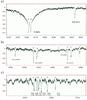 |
Fig. 6 a) PEPSI Hα line profile of HSS 348 (P primary, S secondary). The single diffuse interstellar DIB line at 6613 Å is also marked. b) Doubled Si ii lines from two stellar components appear well separated in this spectrum. The narrow-lined component is the primary, the broad-lined component the secondary. c) Series of Mn ii lines from the primary. |
A number of Mn ii lines are identified following the atlas of the B9V HgMn star HD 175640 (Castelli & Hubrig 2004), e.g., λ7432.3, λ7415.8, a series of lines around λ5292–5302 Å (Fig. 6c) or the four lines at λ6126–6132 Å. These Mn lines appear only from the primary. No Hg line is traceable at our S/N. A single line of gallium is identified as Ga ii λ6334, also only from the primary (see Fig. 6b).
The Na D1,2 doublet appears fully saturated with a flat line core. It is obviously of interstellar origin and related to the column density of sodium in interstellar clouds along the photon path. Hobbs (1974) obtained an empiric calibration of the interstellar D2 (5890 Å) EW with distance. If the measured EW of WD2 = 785 ± 10 mÅ for HSS 348 is indeed all due to interstellar absorption, then the Hobbs relation suggests a distance of around 1 kpc. However, IC 4756 sits in a patchy dust environment according to the available micrometer-emission maps (see Paper I) of which parts are due to the cluster and its foreground. The 1 kpc value is in disagreement with the cluster distance of 440 pc (van Leeuwen 2007) despite its relatively large errors. Both D lines have a sharp redshifted component, indicating the kinematics of the intervening absorption material and it may very well be inappropriate to relate the total EW with only a single distance. No photospheric Na D1,2 wings from HSS 348 are seen, but they would be blended in the broad interstellar absorption.
The K i 7699 doublet appears unsaturated and with a residual line intensity of 30% with respect to the (joint) continuum and shows the same structured profile as Na D. Its total EW is 164 mÅ and also in agreement with a distance of almost 1 kpc according to the calibration of Hobbs (1974). Its profile appears split into a blue and a red component separated by ≈0.28 Å. The red component being almost twice as strong as the blue component, again indicating complex kinematics of the intervening material. The prominent diffuse interstellar band (DIB) lines at λ5780, 5797, and 6613 Å have average EWs of ≈500, 112, and 230 mÅ, respectively (see Fig. 6 for λ6613). The strongest DIB in HSS 348 is the blend at 6284 Å with significantly more than 500 mÅ indicating a considerable column density. Many more features are detected but are comparably weak and were not measured.
The red end of our spectra is dominated by the broad and shallow Paschen lines at λ8598 (P14), λ8665 (P13), and λ8751 Å (P12), again indicating a hot (dwarf) spectrum. Higher Paschen lines (up to P17) are traceable but are very weak and partly buried in the noise, no evidence is seen for the series convergence. The Paschen lines blend with the infrared triplet of Ca ii from which we see no direct evidence in agreement with a late-B or early A-type spectrum rather than an F-type spectrum. No Ca ii H&K emission is evident either.
By far the strongest emission lines in the spectrum are the forbidden oxygen lines [O i] at λ5577, 6300, and 6364 Å with line intensities relative to the continuum of up to 5, 4.5, and 2.3, respectively. The line wavelengths remain stable but their intensities vary by many factors from night to night. The changes are perfectly consistent for the three lines and are paralleled sometimes with geo-coronal emission blue- or redward of the Na i D absorption lines, suggesting that the [O i] emission is also of geo-coronal origin.
4.2. Radial velocities and orbit
The STELLA radial velocities in the appendix were determined from a simultaneous cross-correlation of 24 échelle orders covering 475 to 795 nm with a synthetic spectrum similar to the target properties of both components. We chose a B-star template with Teff = 15 000 K, log g = 5 and [M/H] = 0.0. It gives a good approximation to the line strengths of the O i triplet lines and several of the singly ionized lines, but it appears too deep and too broad at Hα. Radial velocities are variable with a full amplitude of ≈160 km s-1.
We first determine an orbit for both components separately and then combine the two and give rms values for both. We solve for the components using a general least-square fitting algorithm MPFIT (Markwardt 2009) and the prescription from Danby & Burkardt (1983) to calculate the eccentric anomaly for non-zero eccentricity (see Weber & Strassmeier 2011, for a more detailed description). The velocities of the secondary around the two conjunctions were discarded by applying 3-σ clipping. The RV time coverage is a little over one year. The resulting elements and their errors are summarized in Table 5. We derive the final element uncertainties by scaling the one-sigma errors from the covariance matrix using the measured χ2 value. T0 is a time of periastron. We note that the primary RVs show now evidence of the Rossiter-McLaughlin effect due to an eclipse with the secondary.
Orbital elements.
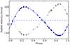 |
Fig. 7 Double-lined STELLA orbit for HSS 348. The primary is the sharper-lined component (full symbols), the secondary is the broader-lined component (open symbols). The dashed line marks the systemic velocity. Typical error bars are smaller than or on the order of the symbol size. |
The computed RV curves are compared with our observed velocities in Fig. 7. Strassmeier et al. (2015a) redetermined the average cluster velocity of IC 4756 from 21 members to −24.0 km s-1 with a rms of around the mean of just ±1.3 km s-1. Our systemic velocity of HSS 348 is in gross disagreement with this (γ = + 21.8 km s-1) and we must conclude that HSS 348 is not a member of IC 4756 and most likely a background target.
Using the orbital inclination of i = 83.4° from the transit analysis, and using the error values for e, T0, and ω from Table 5, the closest encounter of the two components occurs at an orbital phase Φ0 = 0.040 ± 0.005. This is in agreement with the observed eclipse phases of Φ = 0.047 ± 0.004 and suggests that the “transit” is nothing else than a grazing eclipse with the primary star in front. Figure 8 is a schematic graphic representation for the times around the ascending node. We also note that the orbit predicts the absence of a secondary eclipse due to the combination of radii, orbital high eccentricity, its Ω angle, and the inclination, just like the CoRoT observations indicated.
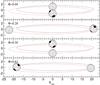 |
Fig. 8 Sketch of the eclipse geometry of HSS 348. Shown are the positions of the primary and the secondary star during the four main phases of the RV curve. During the eclipse at Φ ≈ 0.04 the primary is in front. The spots are only on the primary but see text. All units are in solar radii. |
5. Astrophysical parameters
Summary of astrophysical parameters of HSS 348.
We employed five selected échelle orders per SES spectrum and our synthesis code ParSES (Jovanovic et al. 2013) to determine the effective temperature, gravity, metallicity and projected rotational velocity by iteratively fitting a suite of synthetic spectra (see, e.g., Strassmeier et al. 2013). The final values per spectral order were chosen on the basis of a weighted least-squares fit with three free parameters (Teff, log g, [M/H]) and with fixed values for vsini, micro- and macroturbulence. The details of the method and the numerical tools were described in Allende-Prieto et al. (2004). The mean of the means of all selected orders from a total of 39 spectra for the primary and 27 for the secondary comprise then the best values for each of the three parameters. These values are listed in Table 6. The metallicities of the two HSS 348 stars remain rather uncertain with a rms of 0.5 dex but are consistent with solar metallicity. We find Teff = 12 900 ± 600 K, log g = 4.4 ± 0.3, and solar metallicity for the primary suggesting a B7-8 spectral type. The rotational line broadening was predetermined and assumed to be 10 km s-1 (cf. Sect. 4.1) which translates into a radius of 2.46 R⊙ if Prot is 12.47 d, in very good agreement with the expected radius from the mass-radius relation and the transit measure. However, our vsini of 25 km s-1 for the secondary gives a radius from R = Pv that is too large by a factor 2 compared to the mass-radius relation and the transit geometry. It most likely suggests that we did not measure the true vsini of the component but have yet another line-broadening mechanism contributing to the line width (or possibly a disk around the secondary of which, however, we have no direct evidence).
Assuming two nearly identical components, the individual magnitudes would be ≈075 fainter than the combined Tycho V magnitude of 1195. Formally, this would convert into individual absolute visual magnitudes too faint by three magnitudes if at the distance of IC 4756 (440 pc) with its average  . We have concluded in Paper I that the bulk of the dust emission in the IC 4756 direction from the NASA/IPAC and WISE data, for example, must come from behind the cluster. The new recalibrated reddening (Schlafly & Finkbeiner 2011) provides an absorption of
  for the exact position of HSS 348, which is higher by two magnitudes than the average cluster AV in the foreground. Adopting this value and a distance of 1 kpc, the individual MV are both ≈0355. According to Gray & Corbally (2009), these MV suggest that the B8.5 components agree well with our spectroscopic result.
The mass ratio of near unity (q = m2/m1 = 0.94) together with the comparable long orbital period of 12.47 d implies a well-detached binary configuration. The Roche lobe of the primary is approximately 15.8 R⊙ (R1/a = 0.385) for an inclination of near 90°. With an expected stellar radius of 2.4 R⊙, the primary would be far inside its Roche lobe, above where mass exchange may occur. We can therefore safely reject the scenario that the out-of-transit light-curve variations are caused by eclipses of two semi-contact or contact stars (the four minima would also have required a pair of binaries).
Doppler-boosting (Maxted et al. 2000; Zucker et al. 2007) may introduce light variations proportional to the radial velocity of the components and thus modulated with the orbital period. However, using the equations derived in Loeb & Gaudi (2003) and our radial velocities from the orbit solution in Table 5, we can immediately estimate the Doppler-boosting contribution to be one order of magnitude below the recorded amplitude of even the fundamental period. Doppler-boosting was reported for other Kepler targets, however, see van Kerkwijk et al. (2010). Ellipticity effects entering the light curve at 2f are also negligible for the HSS 348 system, see above and again Zucker et al. (2007).
The two stars in HSS 348 would be sub-synchronous rotators if we accepted that the CoRoT out-of-eclipse light variations are due to variations from both stars. Because the periods from the four light-curve minima are all harmonics of one fundamental period, which is identical to the transit/eclipse period and itself equalling the spectroscopic orbital period, the rotation period of the two stars must be equal to each other and equal to the fundamental period. The expected pseudo-synchronous rotation period according to Hut (1981) that is due to the orbital eccentricity is so significantly shorter (10.4465 d) that we can safely exclude it. Therefore, the two stars rotate too slowly with respect to their orbital revolution. Several binary systems with HgMn primaries are known to rotate sub-synchronously (Guthrie 1986; see also Hubrig et al. 2012), but it is not clear whether a special initial condition or a loss of angular momentum during contraction toward the ZAMS causes this. The detection of a (albeit weak) longitudinal magnetic field in several HgMn binaries (Hubrig et al. 2012) suggests that it may relate to the loss of angular momentum.
The mass-radius relation for the middle main sequence, R ∝ M0.79, returns R ≈ 2.4 R⊙ for the primary and ≈2.3 R⊙ for the secondary, in good agreement with our spectral classifications. With these values and the orbital elements from Table 5, we may compare the current HSS 348 with respect to expected rotational synchronization. Tassoul & Tassoul (1992) introduced a long-range mechanism for braking a binary star with a radiative envelope through an induced large-scale meridional flow that is due to the elongated shape of a rotating component. The resulting replacement of high angular velocity material with low angular velocity material is even more efficient than viscous friction, braking the star very efficiently. This could be a viable mechanism for our HSS 348 system with its current orbital period of 12 days. Its distance-to-radius ratio for the primary is d/R ≈ 17, and thus the time to synchronize it to the orbital motion is ≈1 Myr according to Tassoul & Tassoul (1992). Under the assumption that we can neglect the eccentricity of HSS 348 of 0.18, we conclude that the HSS 348 stars are likely pre-main sequence or ZAMS stars. Then the system very much resembles the AR Aur binary (Hubrig et al. 2010), but with an orbital period that is three times longer.
6. Summary and conclusions
The systemic RV of the HSS 348 binary is different from the average IC 4756-cluster velocity by approximately 40 km s-1 while its position and proper motions in the tangential plane agree with average cluster values. Interstellar absorption in the Na i D and the K i lines is of a strength expected for a distance of ≈1 kpc, more than twice the distance of IC 4756. This evidence leads to the conclusion that HSS 348 is not a cluster member but a background target showing considerable interstellar absorption.
The detection of a number of Mn ii lines together with O i lines and at least one Ga ii line in the primary spectrum indicate a peculiar chemical surface abundance typical for HgMn stars. Although the secondary does not show any of these lines its spectrum is equally rich in Fe ii and Si ii lines and is of comparable spectral type although somewhat less massive. The mass ratio m2/m1 is 0.94. The system is a SB2 binary with a more slowly rotating B8 HgMn component (the primary) and a more normal B8.5 or B9 star (the secondary) with twice the line broadening. The former component has probably arrived on the ZAMS while the secondary is still pre-main sequence and may host a disk or its remnant. More than two thirds of the HgMn stars are known to belong to spectroscopic binaries (Hubrig & Mathys 1995). The astrophysical parameters of HSS 348 very much resemble those of the eclipsing SB2 binary AR Aurigae which consists of a B9 HgMn primary on the ZAMS and a still-contracting B9.5 pre-main-sequence secondary. Its peculiar primary was found to exhibit an inhomogeneous elemental surface distribution and a strong surface magnetic field. We predict similar for HSS 348.
The orbital period from STELLA RVs is equal to the photometric transit period from CoRoT to within its errors, and almost equal to the fundamental period from the complex out-of-eclipse light-curve variations. This suggests an interlinked origin which we conclude is rotational angular momentum closely linked to the orbital momentum. Because the orbit has a significant eccentricity (0.182 ± 0.0056), the fact that the orbital and rotational periods are equal suggests sub-synchronous rotation for both components. The light variation is therefore most likely caused by surface inhomogeneities on both components. These are typically attributed to the combined effects of a chemically peculiar atmosphere, magnetic fields, accretion from the circumbinary medium, and the dredge-up of low angular-momentum material due to a mild ellipticity effect that may also generate a local surface temperature gradient (e.g., Murphy 2015). A spot model with four longitudinally equidistant (circular) spots on one of the two stellar components fits the observed light curve to the measurement precision. A similar fit quality is achieved when two spots are distributed on both components (which is not surprising because the two components are practically equally bright). A consequence is that we cannot uniquely assign the spots to one of the two stellar components but assume that the HgMn component is more likely the spotted star because of its chemical abnormality. However, it is also possible that the secondary star, very likely still pre-main sequence, is the spotted star and that the “spots” are circumstellar in origin and related to the inhomogeneous remains of a circumstellar disk.
The narrow transits are not caused by an orbiting third body but by a grazing eclipse with the narrow-lined primary star in front. While the target turned out to be an interesting binary on its own its narrow transits in the CoRoT light curve are a classical false positive from a planet hunter’s point of view. This again demonstrates the need to investigate such systems in great detail. An analysis of the shape of the transit light curve suggests an inclination of the system of 83.4° which we also assume to be the most likely inclination of the rotational axes of the two stellar components. The position of the ascending node together with the orbital eccentricity and inclination just happened to be such that there will be no secondary eclipses. As a result of the eccentricity of 0.18, periastron passage takes place at phase ≈0.04 and coincides well with the position of one of the four spots. Magnetic field measurements would be extremely helpful for reconstructing the origin of these spots and their gravitationally coupling to the orbital periastron, and they are planned with the new PEPSI polarimeters at the LBT.
Acknowledgments
STELLA was made possible by funding through the State of Brandenburg (MWFK) and the German Federal Ministry of Education and Research (BMBF). The facility is a collaboration of the AIP in Brandenburg, Germany with the IAC in Tenerife, Spain. We warmly thank our colleagues Gabriel Bihain for help with the WiFSIP data reduction, János Bartus and Katalin Oláh for their spot-modeling insights, and Swetlana Hubrig for discussions concerning HgMn stars in general. The comments from an anonymous referee were very helpful and improved the paper.
References
- Aerts, C., De Mey, K., De Cat, P., & Waelkens, C. 1998, in A Half-Century of Stellar Pulsation Interpretations, eds. P. A. Bradley, & J. A. Guzik, ASP Conf. Ser., 135, 380 [Google Scholar]
- Allende-Prieto, C. 2004, Astron. Nachr., 325, 604 [NASA ADS] [CrossRef] [Google Scholar]
- Baglin, A., Auvergne, M., Boisnard, L., et al. 2006, 36th COSPAR Scientific Assembly, 36, 3749 [Google Scholar]
- Balona, L. A. 2013, MNRAS, 431, 2240 [NASA ADS] [CrossRef] [Google Scholar]
- Balona, L. A. 2016, MNRAS, 457, 3724 [NASA ADS] [CrossRef] [Google Scholar]
- Bertin, E., Mellier, Y., Radovich, M., et al. 2002, in The TERAPIX Pipeline, eds. D. A. Bohlender, D. Durand, & T. H. Handley, ASP Conf. Ser., 281, 228 [Google Scholar]
- Bevington, P. R. 1969, in Data Reduction and Error Analysis for the Physical Sciences (New York: McGraw-Hill Book Co.) [Google Scholar]
- Cagas, P., & Pejcha, O. 2012, A&A, 544, L3 [NASA ADS] [CrossRef] [EDP Sciences] [Google Scholar]
- Carone, L., Gandolfi, D., Cabrera, J., et al. 2012, A&A, 538, A112 [NASA ADS] [CrossRef] [EDP Sciences] [Google Scholar]
- Castelli, F., & Hubrig, S. 2004, A&A, 425, 263 [NASA ADS] [CrossRef] [EDP Sciences] [Google Scholar]
- Collins, G. W., Truax, R. J., & Cranmer, S. R. 1991, ApJS, 77, 541 [NASA ADS] [CrossRef] [Google Scholar]
- Danby, J. M. A., & Burkardt, T. M. 1983, Celest. Mech., 31, 95 [NASA ADS] [CrossRef] [Google Scholar]
- Deleuil, M., Meunier, J. C., Moutou, C., et al. 2009, AJ, 138, 649 [NASA ADS] [CrossRef] [Google Scholar]
- Donati, J.-F., Howarth, I. D., Jardine, M., et al. 2006, MNRAS, 370, 629 [NASA ADS] [CrossRef] [Google Scholar]
- Fekel, F. C. 2003, PASP, 115, 807 [NASA ADS] [CrossRef] [Google Scholar]
- Fernandez, J. M., Latham, D. W., Torres, G., et al. 2009, ApJ, 701, 764 [NASA ADS] [CrossRef] [Google Scholar]
- Gerry, P. A. 1991, Anal. Chem., 63, 534 [CrossRef] [Google Scholar]
- Graczyk, D., Soszynski, I., Poleski, R., et al. 2011, Acta Astron., 61, 103 [NASA ADS] [Google Scholar]
- Gray, R. O., & Corbally, J. C. 2009, in Stellar spectral classification (Princeton: Princeton University Press) [Google Scholar]
- Guthrie, B. N. G. 1986, MNRAS, 220, 559 [NASA ADS] [Google Scholar]
- Hanuschik, R. W. 2003, A&A, 407, 1157 [NASA ADS] [CrossRef] [EDP Sciences] [Google Scholar]
- Harmanec, P., Hadrava, P., Yang, S., et al. 1997, A&A, 319, 867 [NASA ADS] [Google Scholar]
- Hauck, B., & Mermilliod, M. 1998, A&AS, 129, 431 [NASA ADS] [CrossRef] [EDP Sciences] [Google Scholar]
- Henry, G. W., Fekel, F. C., Henry, S. M., & Hall, D. S. 2000, ApJS, 130, 201 [NASA ADS] [CrossRef] [Google Scholar]
- Herzog, A. D., Sanders, W. L., & Seggewiss, W. 1975, A&AS, 19, 211 [NASA ADS] [Google Scholar]
- Helminiak, K. G., Graczyk, D., Konacki, M., et al. 2015, MNRAS, 448, 1945 [NASA ADS] [CrossRef] [Google Scholar]
- Hobbs, L. M. 1974, ApJ, 191, 381 [NASA ADS] [CrossRef] [Google Scholar]
- Høg, E., Fabricius, C., Makarov, V. V., et al. 2000, A&A, 355, L27 [NASA ADS] [Google Scholar]
- Hubrig, S., & Mathys, G. 1995, Comments Astrophys., 18, 167 [Google Scholar]
- Hubrig, S., Savanov, I., Ilyin, I., et al. 2010, MNRAS, 408, L61 [NASA ADS] [CrossRef] [Google Scholar]
- Hubrig, S., González, J. F., Ilyin, I., et al. 2012, A&A, 547, A90 [NASA ADS] [CrossRef] [EDP Sciences] [Google Scholar]
- Hut, P. 1981, A&A, 99, 126 [NASA ADS] [Google Scholar]
- Ibanoglu, C., Evren, S., Tas, G., et al. 2009, MNRAS, 392, 757 [NASA ADS] [CrossRef] [Google Scholar]
- Jarque, C. M., & Bera, A. K. 1987, Intern. Statistic Rev., 55, 163 [Google Scholar]
- Johnson, J. A., Apps, K., Zachary Gazak, J., et al. 2011, ApJ, 730, 79 [NASA ADS] [CrossRef] [Google Scholar]
- Jovanovic, M., Weber, M., & Allende-Prieto, C. 2013, Publ. Astron. Obs. Belgrade, 92, 169 [NASA ADS] [Google Scholar]
- Lehmann, H., Zechmeister, M., Dreizler, S., Schuh, S., & Kanzler, R. 2012, A&A, 541, A105 [NASA ADS] [CrossRef] [EDP Sciences] [Google Scholar]
- Lenz P., & Breger M., 2004, in The A-Star Puzzle, eds. J. Zverko, J. Ziznovsky, S. J. Adelman, & W. W. Weiss (Cambridge Univ. Press), IAU Symp., 224, 786 [Google Scholar]
- Loeb, A., & Gaudi, B. S. 2003, ApJ, 588, L117 [NASA ADS] [CrossRef] [Google Scholar]
- Maceroni, C., Montalbán, J., Michel, E., et al. 2009, A&A, 508, 1375 [NASA ADS] [CrossRef] [EDP Sciences] [Google Scholar]
- Mallonn, M., Nascimbeni, V., Weingrill, J., et al. 2015, A&A, 583, A138 [NASA ADS] [CrossRef] [EDP Sciences] [Google Scholar]
- Markwardt, C. B., 2009, in Astronomical Data Analysis Software and Systems XVIII, eds. D. A. Bohlender, D. Durand, & P. Dowler, ASP Confer. Ser., 411, 251 [Google Scholar]
- Maxted, P. F. L., Marsh, T. R., & North, R. C. 2000, MNRAS, 317, L41 [NASA ADS] [CrossRef] [Google Scholar]
- Mermilliod, J. C., Mayor, M., & Udry, S. 2008, A&A, 485, 303 [NASA ADS] [CrossRef] [EDP Sciences] [Google Scholar]
- Murphy, S. J. 2015, Investigating the A-Type Stars Using Kepler Data (Springer Theses), DOI: 10.1007/978-3-319-09417-5_2 [Google Scholar]
- Paparó, M., Chadid, M., Chapellier, E., et al. 2011, A&A, 531, A135 [NASA ADS] [CrossRef] [EDP Sciences] [Google Scholar]
- Pawlak, M., Graczyk, D., Soszynski, I., et al. 2013, Acta Astron., 63, 323 [NASA ADS] [Google Scholar]
- Pietrzynski, G., Thompson, I. B., Gieren, W., et al. 2012, Nature, 484, 75 [NASA ADS] [CrossRef] [PubMed] [Google Scholar]
- Randich, S., Singh, K. P., Simon, T., Drake, S. A., & Schmitt, J. H. M. M. 1998, A&A, 337, 372 [NASA ADS] [Google Scholar]
- Ribárik, G., Oláh, K., & Strassmeier, K. G. 2003, Astron. Nachr., 324, 202 [NASA ADS] [CrossRef] [Google Scholar]
- Roeser, S., Demleitner, M., & Schilbach, E. 2010, AJ, 139, 2440 [NASA ADS] [CrossRef] [Google Scholar]
- Robichon, N., Arenou, F., Mermilliod, J.-C., & Turon, C. 1999, A&A, 345, 471 [NASA ADS] [Google Scholar]
- Samadi, R., Fialho, F., Costa, J. E. S., et al. 2006, ESA SP, 1306, 317 [Google Scholar]
- Schlafly, E. F., & Finkbeiner, D. P. 2011, ApJ, 737, 103 [NASA ADS] [CrossRef] [Google Scholar]
- Sing, D. K. 2010, A&A, 510, A21 [Google Scholar]
- Southworth, J., Maxted, P. F. L., & Smalley, B. 2004, MNRAS, 351, 1277 [NASA ADS] [CrossRef] [Google Scholar]
- Southworth, J., Smalley, B., Maxted, P. F. L., Claret, A., & Etzel, P. B. 2005, MNRAS, 363, 529 [NASA ADS] [CrossRef] [Google Scholar]
- Southworth, J., Bruntt, H., & Buzasi, D. L. 2007, A&A, 467, 1215 [NASA ADS] [CrossRef] [EDP Sciences] [Google Scholar]
- Southworth, J., Mancini, L., Ciceri, S., et al. 2015, MNRAS, 447, 711 [NASA ADS] [CrossRef] [Google Scholar]
- Strassmeier, K. G. 2009, A&ARv, 17, 251 [NASA ADS] [CrossRef] [Google Scholar]
- Strassmeier, K. G., Granzer, T., Weber, M., et al. 2004, Astron. Nachr., 325, 527 [NASA ADS] [CrossRef] [Google Scholar]
- Strassmeier, K. G., Granzer, T., Weber, M., et al. 2010, Adv. in Astr., 2010, 19 [Google Scholar]
- Strassmeier, K. G., Weber, M., Granzer, T., & Järvinen, S. 2012, Astron. Nachr., 333, 663 [NASA ADS] [CrossRef] [Google Scholar]
- Strassmeier, K. G., Weber, M., & Granzer, T. 2013, A&A, 559, A17 [NASA ADS] [CrossRef] [EDP Sciences] [Google Scholar]
- Strassmeier, K. G., Weingrill, J., Granzer, T., et al. 2015a, A&A, 580, A66 (Paper I) [NASA ADS] [CrossRef] [EDP Sciences] [Google Scholar]
- Strassmeier, K. G., Ilyin, I., Jaervinen, A., et al. 2015b, Astron. Nachr., 336, 324 [NASA ADS] [CrossRef] [Google Scholar]
- Tassoul, J.-L., & Tassoul, M. 1992, ApJ, 395, 259 [NASA ADS] [CrossRef] [Google Scholar]
- van Leeuwen, F. 2007, A&A, 474, 653 [NASA ADS] [CrossRef] [EDP Sciences] [Google Scholar]
- van Kerkwijk, M. H., Rappaport, S. A., Breton, R. P., et al, 2010, ApJ, 715, 51 [NASA ADS] [CrossRef] [Google Scholar]
- Weber, M., & Strassmeier, K. G. 2011, A&A, 531, A89 [NASA ADS] [CrossRef] [EDP Sciences] [Google Scholar]
- Weber, M., Granzer, T., Strassmeier, K. G., & Woche, M. 2008, Proc. SPIE, 7019, 70190 [Google Scholar]
- Weingrill, J. 2015, Astron. Nachr., 336, 125 [NASA ADS] [CrossRef] [Google Scholar]
- Winn, J. N., Holman, M. J., Torres, G., et al. 2008, ApJ, 683, 1076 [NASA ADS] [CrossRef] [Google Scholar]
- Zacharias, N., Monet, D. G., Levine, S. E., et al. 2005, Vizier Online Data Catalog: I/297 [Google Scholar]
- Zucker, S., Mazeh, T., & Alexander, T. 2007, ApJ, 670, 1326 [NASA ADS] [CrossRef] [Google Scholar]
Appendix A: Radial velocities from the STELLA/SES follow-up spectroscopy
Barycentric radial velocities of HSS 348.
Appendix B: Observing log for the follow-up STELLA/WiFSIP photometry
STELLA/WiFSIP observing log.
Appendix C: A representative STELLA/SES spectrum
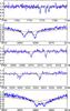 |
Fig. C.1 Sample STELLA/SES spectrum of HSS 348. Shown are five selected spectral features used for determining the component’s radial velocities; from top to bottom, the O i triplet, Hα, Si ii 6372 Å, Si ii 5041 Å, and Hβ. The two lines are synthetic spectra of the two component stars. Both spectra are shifted in wavelength to fit the observed spectrum. |
All Tables
Eight strongest overtones recovered with a fundamental period P0 = 12.4734940 ± 0.000067 d.
All Figures
|
Fig. 1 CoRoT light curve of HSS 348. The time coverage is 173 consecutive days. Thirteen transits were covered. Note the periodic stellar light variations with four unequally deep minima but commensurable period. The brightness zero point is set arbitrarily to the Tycho V-band magnitude. |
| In the text | |
|
Fig. 2 CoRoT PSF footprint overlaid on a stacked STELLA WiFSIP CCD image. The CCD image is obtained with the Johnson V filter and has a limiting magnitude of 21 |
| In the text | |
|
Fig. 3 Thirteen eclipse events phase folded and binned in 30 s intervals, and overplotted with the best-fit model (line). In the lower panel the residuals are shown with an rms of 0.47 mmag. We note that in this plot the orbital phase is centered on the mid-time of the eclipse. |
| In the text | |
|
Fig. 4 Out-of-transit light curve folded with the fundamental period of P0 = 12.473490 ± 0.000067 d recovered from a twelve-component Fourier-series fit (line). Only every fourth data point is plotted. Eclipse points are removed. Orbital phase is according to the elements in Table 5. We note that periastron at the eclipse mid-time takes place at 0 |
| In the text | |
|
Fig. 5 Four-spot light-curve fit. Left: phased CoRoT light curve (the white line is the SML fit and the small dots are the CoRoT data from Fig. 1). Right: spot model in Mercator representation (from left to right identified as spots 1, 2, 3, and 4, see Table 4). We note that the phases of the four light-curve minima do not coincide with the central longitudes of the four spots but that the recovered spot longitudes agree with a time of periastron passage at phase 0 |
| In the text | |
|
Fig. 6 a) PEPSI Hα line profile of HSS 348 (P primary, S secondary). The single diffuse interstellar DIB line at 6613 Å is also marked. b) Doubled Si ii lines from two stellar components appear well separated in this spectrum. The narrow-lined component is the primary, the broad-lined component the secondary. c) Series of Mn ii lines from the primary. |
| In the text | |
|
Fig. 7 Double-lined STELLA orbit for HSS 348. The primary is the sharper-lined component (full symbols), the secondary is the broader-lined component (open symbols). The dashed line marks the systemic velocity. Typical error bars are smaller than or on the order of the symbol size. |
| In the text | |
|
Fig. 8 Sketch of the eclipse geometry of HSS 348. Shown are the positions of the primary and the secondary star during the four main phases of the RV curve. During the eclipse at Φ ≈ 0.04 the primary is in front. The spots are only on the primary but see text. All units are in solar radii. |
| In the text | |
|
Fig. C.1 Sample STELLA/SES spectrum of HSS 348. Shown are five selected spectral features used for determining the component’s radial velocities; from top to bottom, the O i triplet, Hα, Si ii 6372 Å, Si ii 5041 Å, and Hβ. The two lines are synthetic spectra of the two component stars. Both spectra are shifted in wavelength to fit the observed spectrum. |
| In the text | |
Current usage metrics show cumulative count of Article Views (full-text article views including HTML views, PDF and ePub downloads, according to the available data) and Abstracts Views on Vision4Press platform.
Data correspond to usage on the plateform after 2015. The current usage metrics is available 48-96 hours after online publication and is updated daily on week days.
Initial download of the metrics may take a while.