| Issue |
A&A
Volume 597, January 2017
|
|
|---|---|---|
| Article Number | A121 | |
| Number of page(s) | 18 | |
| Section | Interstellar and circumstellar matter | |
| DOI | https://doi.org/10.1051/0004-6361/201628079 | |
| Published online | 13 January 2017 | |
The connection between supernova remnants and the Galactic magnetic field: An analysis of quasi-parallel and quasi-perpendicular cosmic-ray acceleration for the axisymmetric sample
Dept of Physics and Astronomy, University of Manitoba, Winnipeg, R3T 2N2, Canada
e-mail: This email address is being protected from spambots. You need JavaScript enabled to view it.
; This email address is being protected from spambots. You need JavaScript enabled to view it.
Received: 5 January 2016
Accepted: 9 September 2016
Abstract
The mechanism for the acceleration of cosmic-rays in supernova remnants (SNRs) is an outstanding question in the field. We model a sample of 32 axisymmetric SNRs using the quasi-perpendicular and quasi-parallel cosmic-ray-electron (CRE) acceleration cases. The axisymmetric sample is defined to include SNRs with a double-sided, bilateral morphology, and also those with a one-sided morphology where one limb is much brighter than the other. Using a coordinate transformation technique, we insert a bubble-like model SNR into a model of the Galactic magnetic field. Since radio emission of SNRs is dominated by synchrotron emission and since this emission depends on the magnetic field and CRE distribution, we are able to simulate the SNR emission and compare this to data. We find that the quasi-perpendicular CRE acceleration case is much more consistent with the data than the quasi-parallel CRE acceleration case, with G327.6+14.6 (SN1006) being a notable exception. We propose that SN1006 may be a case where both quasi-parallel and quasi-perpendicular acceleration are simultaneously at play in a single SNR.
Key words: ISM: supernova remnants / ISM: magnetic fields / cosmic rays / radio continuum: ISM / polarization
Canada Research Chair.
© ESO, 2017
1. Introduction
The mechanism for acceleration of cosmic-rays in supernova remnants (SNRs) is an outstanding question in the field. A popular idea is that the distribution of the cosmic-ray electrons (CREs) is responsible for determining the morphology of the so-called, bilateral SNRs (e.g., Petruk et al. 2009; Bocchino et al. 2011; Reynoso et al. 2013). These are shell-type SNRs with two lobes of emission, separated by a symmetry axis. It has been long observed that many SNRs exhibit this type of morphology (e.g., Kesteven & Caswell 1987).
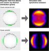 |
Fig. 1 Geometry of CRE distributions for quasi-perpendicular shocks (top) and quasi-parallel shocks (bottom), and the corresponding simulated synchrotron emission, which has been normalized for display purposes. This cartoon is intended to qualitatively show the distribution of the CREs with respect to the magnetic field geometry. It is not intended to be representative of the precise quantitative distributions. |
There are primarily two acceleration scenarios that are considered in the literature: quasi-perpendicular, where CREs are most efficiently accelerated when the shock normal is perpendicular to the post-shock magnetic field; and quasi-parallel where CREs are most efficiently accelerated when the shock normal is parallel to the post-shock magnetic field (Jokipii 1982; Leckband et al. 1989; Fulbright & Reynolds 1990, and references therein). The morphology of these two cases differs in that the axis of bilateral symmetry of the radio synchrotron emission is rotated by 90° with respect to the direction of the ambient magnetic field. In the quasi-perpendicular case, the axis of bilateral symmetry is aligned with the ambient field, whereas in the quasi-parallel case the axis of bilateral symmetry is perpendicular to the ambient field as illustrated in Fig. 1.
One of the main conclusions of Fulbright & Reynolds (1990) was that models of the quasi-parallel scenario produces images that are unlike any observed SNRs and thus, this study was supportive of the quasi-perpendicular case. Several studies since then have looked at these two cases, but there is disagreement about which case is favored. For example, Petruk et al. (2011) pointed out that the odd morphologies predicted by Fulbright & Reynolds (1990) would be expected to be fainter and less likely to be observed. Most of these recent studies have focused on G327.6+14.6 (SN1006), which is one of the brightest SNRs with multi-wavelength data of excellent quality across the electromagnetic spectrum. This well-studied, historical-type SNR has one of the most clearly defined bilateral structure of all SNRs.
Two such studies present evidence in favor of the quasi-perpendicular case: Petruk et al. (2009), who compare the azimuthal brightness profile of radio maps to models, concluding that quasi-perpendicular injection is favored, and Schneiter et al. (2010), who compare both radio and X-ray emission to magnetohydrodynamics (MHD) models to conclude that the Galactic magnetic field (GMF) is most likely perpendicular to the Galactic plane.
Conversely, several other studies are supportive of the quasi-parallel scenario. These include Rothenflug et al. (2004), who suggest that the quasi-parallel scenario is a better fit on the basis of a geometrical argument regarding the limb-to-center brightness ratios; Bocchino et al. (2011), who compare the radio morphology to 3D MHD simulations and conclude that the bright limbs are polar caps; and most recently Schneiter et al. (2015) who focus on a comparison of Stokes Q data to models of this polarization parameter. The addition of this observable lead these authors to support the quasi-parallel case.
Simulations of diffusive shock acceleration (e.g., Matsumoto et al. 2012; 2013; Caprioli & Spitkovsky 2014a) show that electrons are more efficiently accelerated in quasi-perpendicular shocks, whereas protons and other nuclei are more efficiently accelerated in quasi-parallel shocks. It has therefore been proposed that large, turbulent magnetic fields would be expected downstream of parallel shocks, and simple compressed fields in the case of quasi-perpendicular shocks. For SN1006, these authors argue that the observations of Reynoso et al. (2013) agree with their findings and favor the quasi-parallel polar-cap scenario of SN1006. However, they also point out that further, detailed, multi-wavelength observations are necessary to conclusively prove this scenario.
As pointed out above, most studies on this topic in the context of SNRs have focused on SN1006 and we find no studies that undertake a global study of these two CRE acceleration scenarios in the context of many other SNRs with a similar bilateral appearance.
In this paper, we extend the work of West et al. (2016, hereafter Paper I), which presents a detailed study of the radio morphology of 33 clearly defined SNRs with axisymmetric appearance, which includes double-sided bilateral shells as well as one-sided shells where one limb is much brighter than the other, and addresses whether this morphology can be reproduced by modeling the appearance of these SNRs as being the result of compression of the Galactic magnetic field (GMF). Assuming an isotropic CRE distribution, Paper I finds a remarkable agreement (about 75%) between SNR morphology and the model appearance when using the model of Jansson & Farrar (2012, hereafter JF12), which is a model that includes an X-shaped vertical component. The agreement is much less convincing using the GMF model of Sun et al. (2008), which does not include any vertical component.
Radiation from SNRs at radio wavelengths should be dominated by synchrotron radiation, the intensity of which is dependent on the CRE distribution as well as the magnetic field component that is in the plane of the sky. By using an isotropic CRE distribution, Paper 1 demonstrates that the morphology of clearly defined, axisymmetric SNRs is dominated by the large-scale GMF. However, since an isotropic CRE distribution is not considered to be physically motivated and the quasi-perpendicular and quasi-parallel CRE acceleration scenarios discussed above are usually considered more realistic (e.g., Fulbright & Reynolds 1990), it is important to extend the work of Paper I, and consider the effect that the quasi-perpendicular and quasi-parallel CRE acceleration scenarios have on morphology for nearly the same sample of axisymmetric SNRs (with the exclusion of G001.9+00.3, discussed in the following section).
In Sect. 2 we summarize the modeling, which uses the same procedure as Paper I. In Sect. 3 and Appendix A we present the results and discussion of this modeling. In Sect. 4, we present a case study of SN1006 including further modeling (Sect. 4.1) and discussion (Sect. 4.2). G001.9+00.3, which is a special case similar to SN1006, is discussed in Sect. 4.3. Conclusions are found in Sect. 5.
2. Model
Paper I uses a coordinate transformation technique to insert a bubble-like model SNR into a model of the GMF. Given the assumptions that the SNR is in the Sedov phase and that the magnetic field is frozen into the ambient plasma, this method appropriately drags the magnetic field lines of the GMF into the post-shock configuration. The Hammurabi code 1 (Waelkens et al. 2009) is then used to produce simulated Stokes I, Q, and U radio images, as well as polarized intensity ( ) and polarization angle (
 ), which are then compared to real data.
Images of all known Galactic SNRs are studied to choose the cleanest examples of SNRs with axisymmetric appearance. Of these, 33 SNRs that are distributed around the Galaxy, are chosen and modeled at each of 11 different distances: 0.5, 1, 2, 3, 4, 5, 6, 7, 8, 9, and 10 kpc from the Sun. These images are available on the companion website called supernova remnant models and images at radio frequencies (SMIRF)2. For this work, we divide this sample into two parts: SNRs with a double-limbed bilateral morphology, and those with a single-limb. We make this separation since it can be argued that the single-limb SNRs may be interpreted as a double limb that has merged, which would affect the interpretation of the axial orientation. We therefore divide the sample into two parts so we are able to consider the single- and double-sided objects separately.
We also analyze the ages of the SNRs in our sample. With the exception of G001.9+00.3 and possibly SN1006, all the SNRs (with known ages) are expected to be beyond the ejecta-dominated phase and well into the Sedov-Taylor phase of their evolution. Four of them are thought to be core-collapse (CC) type explosions (see Table A.1), where the mass-loss of the progenitor may have perturbed the surrounding medium and magnetic field. However, with the possible exception of G332.4–00.4, all of these SNRs are old enough and large enough that the compression of the ISM is expected to dominate. Two SNRs are thought to be Type Ia: G001.9+00.3, which is suspected to be Type Ia (Reynolds et al. 2008), and SN1006, which is confirmed to be Type Ia (Schaefer 1996; Winkler et al. 2003, and references therein). These two SNRs are also unique for other reasons (see below) and these are discussed separately in Sect. 4.
We emphasize that the focus is on radio data for the physical reason that we here investigate synchrotron emission from ~GeV electrons. The inclusion of X-ray data complicates the interpretation since the thermal X-ray emitting population might be confused with non-thermal emission from particles having TeV energies. We stress that our modeling here is on the global morphology and applied to a selected sample of clean bilateral shells based on radio data, which does not attempt to model small-scale structures, including knots of emission that would be associated with instabilities in the shock and ejecta clumps, for example (e.g., Wang & Chevalier 2001).
In addition, owing to the availability of large-scale radio surveys, a more complete sample of SNRs is available that is relatively consistent in quality. In the case of X-ray data, no observations are available in many cases (or the data has very poor sensitivity) and when high quality data are available, they often only cover a portion of the SNR. X-ray data should only be taken into consideration when they can be shown to be non-thermal. There are only four such cases in our sample: G001.9+00.3, G028.6–00.1, G156.2+05.7, and SN1006 (Ferrand & Safi-Harb 2012, and references therein).
In G028.6–00.1 and G156.2+05.7 the X-ray emission is diffuse and does not exhibit the same bilateral morphology as is observed in radio. On the other hand, G001.9+00.3 and SN1006 are both very young, and their X-ray emission has a clear bilateral morphology. These SNRs therefore deserve special consideration, and both are discussed in Sect. 4. G001.9+00.3 is the youngest in the sample and has the peculiar property that the brightest areas of X-ray and radio emission are anti-correlated. For this reason, we choose to exclude it from the sample under consideration, thus reducing our total sample size to 32 SNRs.
We use the same method and parameters as in Paper I and refer to that study for these additional details. As in Paper I, we also present results for two GMF models, those of JF12 and Sun et al. (2008).
The previous study assumes the simpler case of an isotropic CRE distribution. For this study we include local acceleration effects, comparing the quasi-perpendicular and quasi-parallel CRE distributions. The most common way to model these two scenarios is to scale the CRE distribution by a factor that depends on the angle between the shock normal and the post-shock magnetic field, φBn2 (see Leckband et al. 1989; Fulbright & Reynolds 1990). In the quasi-parallel case this factor is given by cos2φBn2 and for the quasi-perpendicular case it is sin2φBn2.
The quasi-perpendicular case is sometimes called the “equatorial belt”, where the CREs are distributed around the region where the magnetic field is subject to maximum compression. The quasi-parallel case is sometimes referred to as “polar caps”, since the CREs are distributed near the poles of a compressed magnetic field, as illustrated in Fig. 1.
3. Results and discussion
Paper I describes the process of selecting the sample of SNRs with axisymmetric appearance in detail, which is briefly summarized here. The literature and data archives were searched to collect the best-available radio images of all known SNRs. From these, the cleanest and clearest examples of those with bilateral symmetry were selected. Orlando et al. (2007) showed that asymmetries in bilateral SNRs can be explained by gradients of ambient density or magnetic field strength, and therefore SNRs with a single well-defined limb are also included in the sample, but as mentioned above, in this paper we separate the single- and double-limbed SNRs into separate categories so they can be considered separately.
The results of the modeling are presented in Appendix A. Here we show images of the SNRs in comparison to the models for two CRE distributions, at all distances, and for the GMF of JF12. This Appendix, while quite similar to Appendix D in Paper I, has a very important difference since that figure showed models strictly for the isotropic case. By comparing to Paper I, we can see that in terms of the morphology, the quasi-perpendicular case is very similar to the isotropic case for most models, although some small differences do exist in terms of intensity differences and not overall morphology. More importantly, Appendix A here provides a side-by-side comparison for the quasi-perpendicular and quasi-parallel CRE acceleration cases, which is important to visualize the significant morphological differences between these two cases.
Paper I uses a quantitative analysis to compare the models with the data using the bilateral axis angle, ψ, which is the angle between the axis of bilateral symmetry and the Galactic plane. Through the selection of the sample, the objective is to use only the clearest cases where the axis of bilateral symmetry can be unambiguously identified. For the double-limbed cases, the axis of bilateral symmetry is defined as the line running between the two limbs. The limbs are defined to be the brightest region of radio emission, where a corresponding limb on the other side can be identified. In some cases, only a single limb is visible, where no counterpart can be detected on the opposite side. Here, the symmetry axis is chosen to be parallel to the brightest area of emission. This is based on the assumption that there is a corresponding limb on the opposite side that is not detected. The angle is defined using a by-eye method because the data are messy, with point sources and extraneous emission, and it is therefore difficult to devise an automated method to measure this angle. In this study, ψ is also difficult to define for many of the quasi-parallel models since several of them show a filled-centre morphology, which prevents us from defining the angle of bilateral symmetry (e.g., G016.2–02.7, d = 2 kpc). Therefore, we present the models and images together with a qualitative discussion.
The models show that for the quasi-perpendicular case a reasonable morphological match is achieved between model and data for all cases examined and for some distance from 0.5 to 10 kpc, based on a qualitative comparison. The results for the quasi-parallel case, however, show that there are fewer matches between the models and the observations because the quasi-parallel case produces some strange morphologies that are not matched by any SNR, as was pointed out by Fulbright & Reynolds (1990). In at least 10 out of the 32 cases, we find no reasonable morphological match between the data and the model. We also tested the quasi-parallel case for the GMF model of Sun et al. (2008) and found an even poorer correspondence between the model and data than when compared to the JF12 model shown, which is consistent with the results of Paper I.
The quasi-perpendicular case also has better consistency with published distances. While there are seven cases (G028.6–00.1, G093.3+06.9, G116.9+00.2, G119.5+10.2, G127.1+00.5, G327.6+14.6, and G332.4–00.4) where the quasi-parallel case has a reasonable morphological match, the distances in these cases are inconsistent with the published results. For these cases, the quasi-perpendicular case matches both in morphology and distance. There are three cases (G065.1+00.6, G156.2+05.7, and G332.0+00.2) where the quasi-parallel case is consistent for both morphology and distance, but in the case of G156.2+05.7, the quasi-perpendicular case is also a reasonable match. G065.1+00.6 and G332.0+00.2 are the only two cases where the quasi-parallel case is consistent for both morphology and distance but the quasi-perpendicular case is not. In the case of G065.1+00.6, the best-fit quasi-perpendicular case disagrees with the published distance of 9.0–9.6 kpc (Tian & Leahy 2006), but, this published distance is based on a possible association with HI emission that has yet to be confirmed. See Table A.1 for a summary of the distance results.
We searched the literature to find all available magnetic field observations of this sample of 32 SNRs to compare to the magnetic field predicted by our best fitting models. In Fig. 2, we present the data and the models. In 13 out of 15 cases, the observed magnetic field is more consistent with the quasi-perpendicular model. Moreover, in all but one of these cases, the distance also agrees with the best quasi-perpendicular model within our uncertainty. G065.1+00.6 is again the one case that disagrees in terms of distance, but as discussed above, the published distance to G065.1+00.6 is unconfirmed.
The other cases where the direction of the magnetic field is inconsistent are G046.8–0.3 and G327.6+14.6 (SN1006). For G046.8–0.3, polarization data reveal a radial magnetic field (see Fig. 2), but these data have a much lower resolution than the best available radio image (see image in Fig. A.1). As noted in Paper I, the simulated polarization vector plot using the JF12 model is tangential, but it is interesting that the plot using the Sun et al. (2008) model at the corresponding distance (4 kpc) does show a radial magnetic field (see Fig. 7 of Paper I). The case of SN1006 is discussed in the following section. It should also be noted that only in SN1006 is the magnetic field predicted by the quasi-parallel model at all consistent with the observations.
Overall, these results are consistent with the hypothesis that the morphology of clearly axisymmetric SNRs is the result of quasi-perpendicular shocks in a simple compressed GMF.
Other authors (e.g., Petruk et al. 2009; Rothenflug et al. 2004) have used brightness parameters such as the limb-to-center ratio and the radial brightness profiles as a variable to help distinguish between the two CRE scenarios, and we examine the feasibility of using these parameters in the context of this study.
Rothenflug et al. (2004) use a geometrical argument to claim that the quasi-parallel scenario alone is consistent with observations. They argue that in the quasi-perpendicular scenario, the limb-to-center brightness ratio must be at least 0.5 because emission originates in the equatorial belt around the whole perimeter of the SNR. Since the X-ray observations of SN1006 reveal a ratio lower than this (i.e., 0.3), the authors claim that the quasi-perpendicular scenario is ruled out. However, this study also showed that the radio data of SN1006 has a ratio of 0.7, which is quite different from the X-ray observations. Based on the radio data alone, this ratio is not inconsistent with the quasi-perpendicular scenario. Since this study is focused on radio observations and no non-thermal X-rays are observed in nearly all the SNRs in the sample (see previous section), the limb-to-center brightness ratio is not useful for distinguishing between the two scenarios in the cases we are studying.
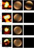 |
Fig. 2 Comparison of the magnetic fields for all cases where a magnetic field has been measured. Magnetic field vectors are plotted on top of the polarized intensity emission. Data (left column) from top to bottom: G016.2–02.7 (Sun et al. 2011a), G021.8–00.6 (Sun et al. 2011a), G046.8–00.3 (Sun et al. 2011a), and G054.4–00.3 (Sun et al. 2011a). Where the data are presented in equatorial coordinates, they are rotated to Galactic coordinates for consistency with the models. Center: best-fit quasi-perpendicular case using the JF12 model. Right: best-fit quasi-parallel case using the JF12 model. In some cases there are no models that match the date reasonably well and the model is shown as blank in these cases. |
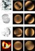 |
Fig. 2 continued. Data (left column) from top to bottom: G065.1+00.6 (Gao et al. 2011), G093.3+06.9 (Milne 1987), G116.9+00.2 (Reich 2002), and G119.5+10.2 (Sun et al. 2011b). |
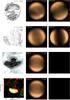 |
Fig. 2 continued. Data (left column) from top to bottom: G127.1+00.5 (Milne 1987), G156.2+05.7 (Reich et al. 1992), G166.0+04.3 (Gao et al. 2011), and G182.4+04.3 (Sun et al. 2011a). |
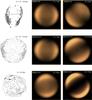 |
Fig. 2 continued. Data (left column) from top to bottom: G296.5+10.0 (Milne 1987), G327.6+14.6 (Reynoso et al. 2013), and G332.4–00.4 (Dickel et al. 1996). |
One other problem with this argument in the context of this study is that the argument of Rothenflug et al. (2004) is only valid for isotropic synchrotron emission found in a region with a disordered magnetic field. In this study, we assume an ordered field, and in addition, its initial orientation might include changes of direction (such as a bend) within the region where the SNR is inserted. For the data, other associated uncertainties in determining the value of the limb-to-center ratio exist as well. This variable might be affected by a non-uniform background level and regions in the ISM of varying density where emission can be enhanced. The localization of these regions is difficult to determine, but it is reasonable to assume that they will not be uniform around the equatorial belt and these enhancements could occur anywhere along the line of sight, in front or behind the SNR. Additionally, all of the radio data in this study are interferometry data, which in many cases lack the addition of short spacing information and therefore affect the limb-to-center ratio. These factors combined with the uncertainty introduced by the directional dependence of the magnetic field on the synchrotron emission means that this parameter is not useful for this study.
Petruk et al. (2009) use azimuthal brightness profiles to favor the quasi-perpendicular scenario, but these profiles can depend on the specific CRE distribution model used. In addition, this model does not account for magnetic field amplification, which is known to modify the non-thermal emission (e.g., Caprioli & Spitkovsky 2014b; Caprioli 2015). For these reasons, the azimuthal brightness is not useful either to distinguish between the two CRE distribution scenarios.
Instead of using these quantitative ratios, this study takes the approach of a qualitative analysis that includes the orientation and magnetic field information.
4. Case study: SN1006
SN1006 is a very bright historical-type SNR with a very well-defined bilateral structure. It has been the subject of many previous studies, and it is therefore important to address this SNR in particular. SN1006 has an observed a diameter of 30′ and a distance of 1.6–2.2 kpc (Ferrand & Safi-Harb 2012, and references therein), although Nikolić et al. (2013) set an upper limit on the distance of 2.1 kpc. The remnant is oriented at an angle of 83° ± 5° with respect to the Galactic plane, which has led to controversy over whether the ambient magnetic field local to SN1006 is oriented perpendicular or parallel to the Galactic plane, depending on whether the quasi-perpendicular or quasi-parallel case is favored by the particular study.
The models presented in Appendix A show that for the quasi-perpendicular case we find a very reasonable morphological fit at a distance of 1±1 kpc, which agrees with the range of published distances and given the uncertainties in the JF12 model. However, for the quasi-parallel case, there is no reasonable fit for any distance modeled, although the 0.5 kpc case is the closest match in terms of orientation.
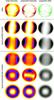 |
Fig. 3 Observations of G327.6+14.6 (SN1006) compared to a selection of grid-based models. The magnetic field is defined by the components Bx (line-of-sight component), By (horizontal component), and Bz (vertical component), where the ratio between the By and Bz-components determines the orientation of the bilateral symmetry axis. Top row: observations of SN1006. Left: Stokes I total intensity (MOST). Center: polarized intensity (Reynoso et al. 2013). Right: magnetic field vectors shown with total intensity contours in the background (adapted from Reynoso et al. 2013). Second row: quasi-parallel model with Bx = 0.03μG, By = 1.0μG, and Bz = 0.12μG. Third row: quasi-parallel model with Bx = 0.55μG, By = 1.0μG, and Bz = 0.12μG. Fourth row: quasi-perpendicular model with Bx = 1.28μG, By = −0.12μG, and Bz = 1.0μG. This is very close to the case at the location of SN1006 in the JF12 GMF model. Fifth row: quasi-perpendicular model with Bx = −3.84μG, By = −0.12μG, and Bz = 1.0μG. Bottom row: quasi-perpendicular model with Bx = −12.5μG, By = −0.12μG, and Bz = 1.0μG. The models are arranged as the data, with far left: Stokes I total intensity; center: polarized intensity, and right: magnetic field vectors shown over total intensity emission. |
4.1. Further modeling of SN1006
Any model of SN1006 must be able to account for all observations, including observations of radio polarization. Reynoso et al. (2013) published detailed observations of this SNR that show that the magnetic field is radial in appearance. The availability of the Stokes Q radio polarization parameter from the observations of Reynoso et al. (2013) lead Schneiter et al. (2015) to model this additional parameter and conclude that the quasi-parallel case was closer to observations than the model for the quasi-perpendicular case. This conclusion, based on these new observations, was contrary to earlier results from the same authors (Schneiter et al. 2010) that supported the quasi-perpendicular case, highlighting the need to include all available observations.
The Hammurabi code also provides model Stokes Q and U images, which together may be used to produce a simulation of the magnetic field vectors that would be observed. We compare our models simultaneously to the following observables: total intensity emission (Stokes I), the polarized intensity emission, and the magnetic field vectors (i.e., polarization angle + 90°).
The JF12 model probably models the global properties of the GMF well, but local variations are not included so it is possible that the model will not be correct at the position of some individual SNRs. If we assume this to be the case for the position of SN1006, then the magnetic field may have some arbitrary configuration. We model SN1006 using a uniform magnetic field that is defined by Bx (line-of-sight component), By (horizontal component), and Bz (vertical component) to find a model that takes all of the observable properties described above into account.
We note that since SN1006 is tilted by 83° with respect to the Galactic plane, the By and Bz components must have a specific relationship for the model SNR to have the same angle. For the quasi-perpendicular case, tan(ψ) = Bz/By and for the quasi-parallel case, tan(ψ) = −By/Bz. For example, in our models of the quasi-parallel case, By is set to 1 μG, which means that Bz must be 0.12 μG to give the correct orientation whereas in the quasi-perpendicular case, Bz is set to 1 μG, which means By must be −0.12 μG for the same reason. The absolute values of By and Bz are not significant; it is the ratios that matter since we are interested in a more qualitative analysis.
By altering the Bx component, we change the limb-to-center brightness ratio and radial brightness profiles. In Fig. 3, we show several quasi-parallel and quasi-perpendicular models that have the correct orientation, but varying values of Bx.
In the quasi-parallel case, Bx must be smaller than By, otherwise the center of SNR is completely filled in and the limbs are not defined. We show two cases that show that the pattern of the magnetic field vectors is radial in the limbs, as in the data, and remains essentially unchanged for all cases where Bx<By.
In the quasi-perpendicular case, the pattern of the magnetic field vectors are tangential to the limbs for most cases, except when the Bx component increases (Fig. 3, bottom row), the magnetic field pattern changes to a radial pattern. The morphology of the polarized intensity emission also changes significantly for this case and becomes inconsistent with the data. The morphology of the emission also changes from bright limbs to ring-like. In Fig. 3, we plot three quasi-perpendicular cases that show this transition from tangential to radial magnetic field and illustrate that it is not possible to match both the intensity pattern and the magnetic field at the same time.
We do not attempt a detailed quantitative optimization of parameters such as comparison of the limb-to-center brightness ratio or radial brightness profiles. Such analyses are done in previous works (see discussion in Sect. 1) with contradictory conclusions as to which CRE acceleration scenario is supported. Instead, we present our models here for qualitative comparison between the morphology together with the magnetic field pattern.
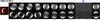 |
Fig. 4 Models of the SNR G001.9+00.3 compared to VLA radio data from Reynolds et al. (2008). The arrow marks the best published distance estimate of 8.5 kpc (Ferrand & Safi-Harb 2012, and references therein). |
4.2. Discussion of SN1006
Our models agree with Schneiter et al. (2015) in that the quasi-parallel model most closely matches the complete set of observations. We therefore conclude that the quasi-parallel case is indeed the better fit for SN1006, which is different from the results for most of the other SNRs in this study. In the majority of the other cases the quasi-perpendicular case yields the better fit.
The quasi-parallel case is not perfect in describing the observations, however. In particular, the magnetic field vectors for the quasi-parallel model converge at the poles but this is not observed in the high-resolution magnetic field vector map by Reynoso et al. (2013).
It may be that SN1006 and possibly G001.9+00.3 as well (discussed below), both being very young SNRs may be different. Young SNRs would be expected to be dominated by turbulence, and it is likely that in these young cases the Rayleigh-Taylor instabilities are playing a major role.
The magnetic fields of SN1006, and other young SNRs, are seen to be amplified at the bright limbs (Bamba et al. 2003, 2004, 2006; Reynolds et al. 2012). Our models have not accounted for this turbulent amplification, nor do those of other authors (e.g., Schneiter et al. 2015). It has been suggested that turbulence can lead to selective amplification of the radial component of the magnetic field (e.g., Inoue et al. 2013). We note that this could alter the observed properties, particularly the polarized emission and observed magnetic-field vectors. This turbulence must not be so significant as to destroy the regular, bilateral appearance, but it may be possible that it imparts the apparent radial magnetic field pattern.
Furthermore, observations of SN1006 show non-thermal X-ray and γ-ray emission (Koyama et al. 1995; Acero et al. 2010) in correspondence to the bright limbs. Caprioli & Spitkovsky (2014a) suggest that the γ-ray emission might indicate ion-acceleration and thus might further support the quasi-parallel scenario given the prediction that ions are more efficiently accelerated in quasi-parallel shocks.
We observe the following:
-
1.
the quasi-parallel case is favored for SN1006;
-
2.
the quasi-perpendicular case is favored for the majority of other axisymmetric SNRs;
-
3.
the JF12 model gives a good fit to the total intensity emission for the quasi-perpendicular CRE case and for a distance that is consistent with other measurements;
-
4.
neither the quasi-parallel nor quasi-perpendicular cases can convincingly reproduce the observed pattern of the magnetic field; and
-
5.
for SN1006, there is disagreement in the literature as to whether the quasi-parallel or quasi-perpendicular CRE case is favored with evidence supporting both scenarios.
We therefore suggest that the regular bilateral morphology of SN1006 may be due to the compressed GMF, and that this compression is around the equatorial belt. The observed radial magnetic field pattern may be imparted by turbulence that does not destroy the morphology that is due to the direction of the regular component of the field.
Additionally, we suggest that both quasi-parallel and quasi-perpendicular acceleration might be simultaneously at play in the same SNR. That is, the initial compression of the GMF leads to quasi-perpendicular acceleration of electrons, which leads to the synchrotron radio emission. Then, turbulence in the young SNR may lead to local magnetic field amplification, which results in a radially oriented magnetic field component. At this point, quasi-parallel acceleration can occur, leading to the acceleration of ions and the γ-ray emission at the limbs, coincident with the radio emission.
4.3. Discussion of G001.9+00.3
G001.9+00.3 is a very young SNR and is thought to be the youngest in the Galaxy at only 150–220 yr (Carlton et al. 2011; Gómez & Rodríguez 2009; Green et al. 2008; Reynolds et al. 2008). It is located at a distance of 8.5 kpc (Reynolds et al. 2008). This SNR has the peculiar property that the brightest areas of X-ray and radio emission are anti-correlated. With the method described above (where the axis of bilateral symmetry is defined as being parallel to the brightest region of radio emission, where a corresponding limb on the other side can be identified) the axis of symmetry would be inclined at a large angle (~−85°), making it nearly vertical. However, the X-ray data (see Reynolds et al. 2008), which in the case of this SNR are mostly non-thermal, clearly show a symmetry axis that is close to parallel with the Galactic plane.
For completeness, we present our models compared to radio data in Fig. 4. The extreme youth of this SNR means that it almost certainly has not reached the Sedov phase of its evolution, making it a unique case where this modeling does not apply.
5. Conclusions
Our results support the conclusion of Fulbright & Reynolds (1990) that the quasi-parallel scenario produces images that are unlike any observed SNRs. We show that the large majority of our models, about 75%, match to the data for the quasi-perpendicular CRE case well, and most are consistent with published distance estimates to the SNRs. In the quasi-parallel CRE case, there is very poor agreement between the appearance of the models and the data. We therefore conclude that the radio morphology of most axisymmetric SNRs is the result of quasi-perpendicular shocks in a simple, compressed GMF.
The SNRs SN1006 and G001.9+00.3 are notable exceptions, and we find for SN1006 that neither of the simple quasi-parallel nor the quasi-perpendicular CRE case can fully describe the observations; although given a single choice, the quasi-parallel CRE case is the better option. Because the JF12 GMF model with the quasi-perpendicular CRE case fits the morphology of SN1006 well at a distance that is consistent with published distance to SN1006, we suggest that the regular radio morphology of this SNR, like the majority of other axisymmetric SNRs, is due to the compressed GMF, and that this compression is around the equatorial belt. The deviations from the quasi-perpendicular model, which includes the observed radial magnetic field pattern, may be imparted by a turbulent magnetic field component that is in addition to the regular magnetic field component. We suggest that SN1006, and possibly other young energetic SNRs that show non-thermal X-ray and γ-ray emission, are examples where both quasi-parallel and quasi-perpendicular acceleration are at play simultaneously.
Acknowledgments
This research was primarily supported by the Natural Sciences and Engineering Research Council of Canada (NSERC) through a Canada Graduate Scholarship (J. West) and the Canada Research Chairs and Discovery Grants Programs (S. Safi-Harb). The modeling was performed on a local computing cluster funded by the Canada Foundation for Innovation (CFI) and the Manitoba Research and Innovation Fund (MRIF). The radio images presented in this paper and companion website made use of data obtained with the following facilities: CHIPASS 1.4 GHz radio continuum map, Canadian Galactic Plane Survey (CGPS) and other data from the Dominion Radio Astrophysical Observatory, Southern Galactic Plane Survey, Effelsberg 100 m Telescope and Stockert Galactic plane survey (2720 MHz; via MPIfR’s Survey Sampler), Molonglo Observatory Synthesis Telescope (MOST) Supernova Remnant Catalogue (843 MHz), Sino-German 6 cm survey. Additionally we acknowledge the use of NASA’s SkyView facility (http://skyview.gsfc.nasa.gov) located at NASA Goddard Space Flight Center for the data from the 4850 MHz Survey/GB6 Survey, NRAO VLA Sky Survey, Sydney University Molonglo Sky Survey (843 MHz), and the Westerbork Northern Sky Survey (325 MHz Continuum). Very Large Array (VLA) data was acquired via the NRAO Science Data Archive and the Multi-Array Galactic Plane Imaging Survey. We thank Michael Bietenholz and David Kaplan for providing the VLA images of G021.6–00.8 and G042.8+00.6, respectively. This research made use of APLpy, an open-source plotting package for Python (http://aplpy.github.com) and Astropy, a community-developed core Python package for Astronomy (Astropy Collaboration 2013). This research also made use of Montage, which is funded by the National Science Foundation under Grant Number ACI-1440620, and was previously funded by the National Aeronautics and Space Administration’s Earth Science Technology Office, Computation Technologies Project, under Cooperative Agreement Number NCC5-626 between NASA and the California Institute of Technology. This research has made use of the NASA Astrophysics Data System (ADS). We thank the referee for comments that improved the manuscript.
References
- Acero, F., Aharonian, F., Akhperjanian, A. G., et al. 2010, A&A, 516, A62 [NASA ADS] [CrossRef] [EDP Sciences] [Google Scholar]
- Astropy Collaboration, Robitaille, P., Tollerud, E. J., et al. 2013, A&A, 558, A33 [NASA ADS] [CrossRef] [EDP Sciences] [Google Scholar]
- Bamba, A., Yamazaki, R., Ueno, M., & Koyama, K. 2003, ApJ, 589, 827 [NASA ADS] [CrossRef] [Google Scholar]
- Bamba, A., Yamazaki, R., Ueno, M., & Koyama, K. 2004, Adv. Space Res., 33, 376 [NASA ADS] [CrossRef] [Google Scholar]
- Bamba, A., Yamazaki, R., Yoshida, T., Terasawa, T., & Koyama, K. 2006, Adv. Space Res., 37, 1439 [NASA ADS] [CrossRef] [Google Scholar]
- Bocchino, F., Orlando, S., Miceli, M., & Petruk, O. 2011, A&A, 531, A129 [NASA ADS] [CrossRef] [EDP Sciences] [Google Scholar]
- Caprioli, D. 2015, ArXiv e-prints [arXiv:1510.07042] [Google Scholar]
- Caprioli, D., & Spitkovsky, A. 2014a, ApJ, 783, 91 [NASA ADS] [CrossRef] [Google Scholar]
- Caprioli, D., & Spitkovsky, A. 2014b, ApJ, 794, 46 [NASA ADS] [CrossRef] [Google Scholar]
- Carlton, A. K., Borkowski, K. J., Reynolds, S. P., et al. 2011, ApJ, 737, L22 [NASA ADS] [CrossRef] [Google Scholar]
- Condon, J. J., Griffith, M. R., & Wright, A. E. 1993, AJ, 106, 1095 [NASA ADS] [CrossRef] [Google Scholar]
- Condon, J. J., Cotton, W. D., Greisen, E. W., et al. 1998, AJ, 115, 1693 [NASA ADS] [CrossRef] [Google Scholar]
- Dickel, J. R., Green, A., Ye, T., & Milne, D. K. 1996, AJ, 111, 340 [NASA ADS] [CrossRef] [Google Scholar]
- Ferrand, G., & Safi-Harb, S. 2012, Adv. Space Res., 49, 1313 [NASA ADS] [CrossRef] [Google Scholar]
- Fulbright, M. S., & Reynolds, S. P. 1990, ApJ, 357, 591 [NASA ADS] [CrossRef] [Google Scholar]
- Gao, X. Y., Reich, W., Han, J. L., et al. 2010, A&A, 515, A64 [NASA ADS] [CrossRef] [EDP Sciences] [Google Scholar]
- Gao, X. Y., Han, J. L., Reich, W., et al. 2011, A&A, 529, A159 [NASA ADS] [CrossRef] [EDP Sciences] [Google Scholar]
- Gómez, Y., & Rodríguez, L. F. 2009, Rev. Mex. Astron. Astrofis., 45, 91 [NASA ADS] [Google Scholar]
- Green, D. A., Reynolds, S. P., Borkowski, K. J., et al. 2008, MNRAS, 387, L54 [NASA ADS] [CrossRef] [Google Scholar]
- Helfand, D. J., Becker, R. H., White, R. L., Fallon, A., & Tuttle, S. 2006, AJ, 131, 2525 [NASA ADS] [CrossRef] [Google Scholar]
- Inoue, T., Shimoda, J., Ohira, Y., & Yamazaki, R. 2013, ApJ, 772, L20 [NASA ADS] [CrossRef] [Google Scholar]
- Jansson, R., & Farrar, G. R. 2012, ApJ, 757, 14 [NASA ADS] [CrossRef] [Google Scholar]
- Jokipii, J. R. 1982, ApJ, 255, 716 [NASA ADS] [CrossRef] [Google Scholar]
- Kesteven, M. J., & Caswell, J. L. 1987, A&A, 183, 118 [NASA ADS] [Google Scholar]
- Koyama, K., Petre, R., Gotthelf, E. V., et al. 1995, Nature, 378, 255 [NASA ADS] [CrossRef] [Google Scholar]
- Landecker, T. L., Routledge, D., Reynolds, S. P., et al. 1999, ApJ, 527, 866 [NASA ADS] [CrossRef] [Google Scholar]
- Leckband, J. A., Spangler, S. R., & Cairns, I. H. 1989, ApJ, 338, 963 [NASA ADS] [CrossRef] [Google Scholar]
- Matsumoto, Y., Amano, T., & Hoshino, M. 2012, ApJ, 755, 109 [NASA ADS] [CrossRef] [Google Scholar]
- Matsumoto, Y., Amano, T., & Hoshino, M. 2013, Phys. Rev. Lett., 111, 215003 [NASA ADS] [CrossRef] [Google Scholar]
- Milne, D. K. 1987, Aust. J. Phys., 40, 771 [NASA ADS] [Google Scholar]
- Nikolić, S., van de Ven, G., Heng, K., et al. 2013, Science, 340, 45 [NASA ADS] [CrossRef] [Google Scholar]
- Orlando, S., Bocchino, F., Reale, F., Peres, G., & Petruk, O. 2007, A&A, 470, 927 [NASA ADS] [CrossRef] [EDP Sciences] [Google Scholar]
- Petruk, O., Dubner, G. M., Castelletti, G., et al. 2009, MNRAS, 393, 1034 [NASA ADS] [CrossRef] [Google Scholar]
- Petruk, O., Orlando, S., Beshley, V., & Bocchino, F. 2011, MNRAS, 413, 1657 [NASA ADS] [CrossRef] [Google Scholar]
- Reich, W. 2002, in Neutron Stars, Pulsars, and Supernova Remnants, eds. W. Becker, H. Lesch, & J. Trümper, 1 [Google Scholar]
- Reich, W., Fuerst, E., & Arnal, E. M. 1992, ApJ, 256, 214 [Google Scholar]
- Rengelink, R. B., Tang, Y., de Bruyn, A. G., et al. 1997, A&AS, 124, 259 [NASA ADS] [CrossRef] [EDP Sciences] [Google Scholar]
- Reynolds, S. P., Borkowski, K. J., Green, D. A., et al. 2008, ApJ, 680, L41 [NASA ADS] [CrossRef] [Google Scholar]
- Reynolds, S. P., Gaensler, B. M., & Bocchino, F. 2012, Space Sci. Rev., 166, 231 [NASA ADS] [CrossRef] [Google Scholar]
- Reynoso, E. M., Hughes, J. P., & Moffett, D. A. 2013, AJ, 145, 104 [NASA ADS] [CrossRef] [Google Scholar]
- Rothenflug, R., Ballet, J., Dubner, G. M., et al. 2004, A&A, 425, 121 [NASA ADS] [CrossRef] [EDP Sciences] [Google Scholar]
- Schaefer, B. E. 1996, ApJ, 459, 438 [NASA ADS] [CrossRef] [Google Scholar]
- Schneiter, E. M., Velázquez, P. F., Reynoso, E. M., & De Colle, F. 2010, MNRAS, 408, 430 [NASA ADS] [CrossRef] [Google Scholar]
- Schneiter, E. M., Velazquez, P. F., Reynoso, E. M., Esquivel, A., & De Colle, F. 2015, MNRAS, 449, 88 [NASA ADS] [CrossRef] [Google Scholar]
- Sun, X. H., Reich, W., Waelkens, A., & Enßlin, T. A. 2008, A&A, 477, 573 [NASA ADS] [CrossRef] [EDP Sciences] [Google Scholar]
- Sun, X. H., Reich, P., Reich, W., et al. 2011a, A&A, 536, A83 [NASA ADS] [CrossRef] [EDP Sciences] [Google Scholar]
- Sun, X. H., Reich, W., Wang, C., Han, J. L., & Reich, P. 2011b, A&A, 535, A64 [NASA ADS] [CrossRef] [EDP Sciences] [Google Scholar]
- Taylor, A. R., Gibson, S. J., Peracaula, M., et al. 2003, AJ, 125, 3145 [NASA ADS] [CrossRef] [Google Scholar]
- Tian, W. W., & Leahy, D. A. 2006, A&A, 455, 1053 [NASA ADS] [CrossRef] [EDP Sciences] [Google Scholar]
- Waelkens, A., Jaffe, T., Reinecke, M., Kitaura, F. S., & Enßlin, T. A. 2009, A&A, 495, 697 [NASA ADS] [CrossRef] [EDP Sciences] [Google Scholar]
- Wang, C.-Y., & Chevalier, R. A. 2001, ApJ, 549, 1119 [NASA ADS] [CrossRef] [Google Scholar]
- West, J. L., Safi-Harb, S., Jaffe, T., et al. 2016, A&A, 587, A148 [NASA ADS] [CrossRef] [EDP Sciences] [Google Scholar]
- Whiteoak, J. B. Z., & Green, A. J. 1996, A&AS, 118, 329 [NASA ADS] [CrossRef] [EDP Sciences] [Google Scholar]
- Winkler, P. F., Gupta, G., & Long, K. S. 2003, ApJ, 585, 324 [NASA ADS] [CrossRef] [Google Scholar]
Appendix A: Data shown in comparison to the models
In Figs. A.1 and A.2 we present models for quasi-perpendicular and quasi-parallel CRE acceleration and compare these to images for the double-sided and single-sided SNRs respectively. In each case the data are shown on the left (image references are summarized in Table A.1).
To the right of the image are two strips of models: the models for the quasi-perpendicular CRE distribution are shown in the top row and the models for the quasi-parallel CRE distribution are shown below. These were made for the position of theparticular SNR and at the various distances as labeled (in kpc). In some cases the Galactic field model is undefined at a location and so the model image shows a blank (see Paper I). The set of best-fitting models, based on the visual appearance of the angle is highlighted with an orange box. In almost one-third of the quasi-parallel cases (G021.8–00.6, G036.6+02.6, G046.8–00.3, G054.4–00.3, G166.0+04.3, G182.4+04.3, G302.3+00.7, G315.1+02.7, G317.3–00.2, and G321.9–00.3) none of the models were judged to have a convincing morphological counterpart and so no model was chosen. Where a published value for the distance is available, the range is indicated by an arrow above the models.
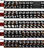 |
Fig. A.1 Data (left) shown in comparison to models at distances of 0.5, 1, 2, 3, 4, 5, 6, 7, 8, 9, and 10 kpc (left to right) showing the quasi-perpendicular (top) and quasi-parallel (bottom) CRE acceleration case for each SNR in the sample with a double limb. The set of best-fitting models, based on the visual appearance of the angle is highlighted with an orange box. In some cases the model is undefined at a location and so the model image show a blank. Where a published value for the distance is available, the range is indicated by an arrow above the models (references for these distances are summarized in Table 1). |
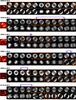 |
Fig. A.1 continued. |
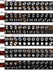 |
Fig. A.1 continued. |
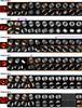 |
Fig. A.1 continued. |
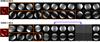 |
Fig. A.1 continued. |
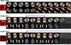 |
Fig. A.2 Data (left) shown in comparison to models at distances of 0.5, 1, 2, 3, 4, 5, 6, 7, 8, 9, and 10 kpc (left to right) showing the quasi-perpendicular (top) and quasi-parallel ( bottom) CRE acceleration case for each SNR in the sample with a single limb. In some cases the model is undefined at a location and so the model image will show a blank. Where a published value for the distance is available, the range is indicated by an arrow above the models (references for these distances are summarized in Table A.1). |
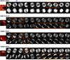 |
Fig. A.2 continued. |
Summary of the published parameters for the SNRs shown with distance ranges corresponding to models with a reasonable morphological match.
All Tables
Summary of the published parameters for the SNRs shown with distance ranges corresponding to models with a reasonable morphological match.
All Figures
|
Fig. 1 Geometry of CRE distributions for quasi-perpendicular shocks (top) and quasi-parallel shocks (bottom), and the corresponding simulated synchrotron emission, which has been normalized for display purposes. This cartoon is intended to qualitatively show the distribution of the CREs with respect to the magnetic field geometry. It is not intended to be representative of the precise quantitative distributions. |
| In the text | |
|
Fig. 2 Comparison of the magnetic fields for all cases where a magnetic field has been measured. Magnetic field vectors are plotted on top of the polarized intensity emission. Data (left column) from top to bottom: G016.2–02.7 (Sun et al. 2011a), G021.8–00.6 (Sun et al. 2011a), G046.8–00.3 (Sun et al. 2011a), and G054.4–00.3 (Sun et al. 2011a). Where the data are presented in equatorial coordinates, they are rotated to Galactic coordinates for consistency with the models. Center: best-fit quasi-perpendicular case using the JF12 model. Right: best-fit quasi-parallel case using the JF12 model. In some cases there are no models that match the date reasonably well and the model is shown as blank in these cases. |
| In the text | |
|
Fig. 2 continued. Data (left column) from top to bottom: G065.1+00.6 (Gao et al. 2011), G093.3+06.9 (Milne 1987), G116.9+00.2 (Reich 2002), and G119.5+10.2 (Sun et al. 2011b). |
| In the text | |
|
Fig. 2 continued. Data (left column) from top to bottom: G127.1+00.5 (Milne 1987), G156.2+05.7 (Reich et al. 1992), G166.0+04.3 (Gao et al. 2011), and G182.4+04.3 (Sun et al. 2011a). |
| In the text | |
|
Fig. 2 continued. Data (left column) from top to bottom: G296.5+10.0 (Milne 1987), G327.6+14.6 (Reynoso et al. 2013), and G332.4–00.4 (Dickel et al. 1996). |
| In the text | |
|
Fig. 3 Observations of G327.6+14.6 (SN1006) compared to a selection of grid-based models. The magnetic field is defined by the components Bx (line-of-sight component), By (horizontal component), and Bz (vertical component), where the ratio between the By and Bz-components determines the orientation of the bilateral symmetry axis. Top row: observations of SN1006. Left: Stokes I total intensity (MOST). Center: polarized intensity (Reynoso et al. 2013). Right: magnetic field vectors shown with total intensity contours in the background (adapted from Reynoso et al. 2013). Second row: quasi-parallel model with Bx = 0.03μG, By = 1.0μG, and Bz = 0.12μG. Third row: quasi-parallel model with Bx = 0.55μG, By = 1.0μG, and Bz = 0.12μG. Fourth row: quasi-perpendicular model with Bx = 1.28μG, By = −0.12μG, and Bz = 1.0μG. This is very close to the case at the location of SN1006 in the JF12 GMF model. Fifth row: quasi-perpendicular model with Bx = −3.84μG, By = −0.12μG, and Bz = 1.0μG. Bottom row: quasi-perpendicular model with Bx = −12.5μG, By = −0.12μG, and Bz = 1.0μG. The models are arranged as the data, with far left: Stokes I total intensity; center: polarized intensity, and right: magnetic field vectors shown over total intensity emission. |
| In the text | |
|
Fig. 4 Models of the SNR G001.9+00.3 compared to VLA radio data from Reynolds et al. (2008). The arrow marks the best published distance estimate of 8.5 kpc (Ferrand & Safi-Harb 2012, and references therein). |
| In the text | |
|
Fig. A.1 Data (left) shown in comparison to models at distances of 0.5, 1, 2, 3, 4, 5, 6, 7, 8, 9, and 10 kpc (left to right) showing the quasi-perpendicular (top) and quasi-parallel (bottom) CRE acceleration case for each SNR in the sample with a double limb. The set of best-fitting models, based on the visual appearance of the angle is highlighted with an orange box. In some cases the model is undefined at a location and so the model image show a blank. Where a published value for the distance is available, the range is indicated by an arrow above the models (references for these distances are summarized in Table 1). |
| In the text | |
|
Fig. A.1 continued. |
| In the text | |
|
Fig. A.1 continued. |
| In the text | |
|
Fig. A.1 continued. |
| In the text | |
|
Fig. A.1 continued. |
| In the text | |
|
Fig. A.2 Data (left) shown in comparison to models at distances of 0.5, 1, 2, 3, 4, 5, 6, 7, 8, 9, and 10 kpc (left to right) showing the quasi-perpendicular (top) and quasi-parallel ( bottom) CRE acceleration case for each SNR in the sample with a single limb. In some cases the model is undefined at a location and so the model image will show a blank. Where a published value for the distance is available, the range is indicated by an arrow above the models (references for these distances are summarized in Table A.1). |
| In the text | |
|
Fig. A.2 continued. |
| In the text | |
Current usage metrics show cumulative count of Article Views (full-text article views including HTML views, PDF and ePub downloads, according to the available data) and Abstracts Views on Vision4Press platform.
Data correspond to usage on the plateform after 2015. The current usage metrics is available 48-96 hours after online publication and is updated daily on week days.
Initial download of the metrics may take a while.