| Issue |
A&A
Volume 596, December 2016
|
|
|---|---|---|
| Article Number | A17 | |
| Number of page(s) | 14 | |
| Section | Astrophysical processes | |
| DOI | https://doi.org/10.1051/0004-6361/201628931 | |
| Published online | 22 November 2016 | |
A disk wind in AB Aurigae traced with Hα interferometry⋆
1 Université Grenoble Alpes, IPAG, 38000 Grenoble, France
e-mail: karine.perraut@obs.ujf-grenoble.fr
2 CNRS, IPAG, 38000 Grenoble, France
3 Depto de Formação Geral de Contagem, Centro Federal de Educação Tecnológica de Minas Gerais, Brazil
4 Laboratoire Lagrange, Université Côte d’Azur, Observatoire de la Côte d’Azur, CNRS, Bd de l’Observatoire, CS 34229, 06304 Nice Cedex 4, France
5 Aix-Marseille Université, CNRS, LAM, UMR 7326, 13388 Marseille, France
6 Université de Lyon, Université Lyon 1, École Normale Supérieure de Lyon, CNRS, Centre de Recherche Astrophophysique de Lyon UMR 5574, 69230 Saint-Genis-Laval, France
7 CHARA Array, Mount Wilson Observatory, Mount Wilson, CA 91023, USA
Received: 13 May 2016
Accepted: 11 July 2016
Context. A crucial issue in star formation is understanding the physical mechanism by which mass is accreted onto and ejected by a young star, then collimated into jets. Hydrogen lines are often used to trace mass accretion in young stars, but recent observations suggest that they could instead trace mass outflow in a disk wind.
Aims. Obtaining direct constraints on the HI line formation regions is crucial in order to disentangle the different models. We present high angular and spectral resolution observations of the Hα line of the Herbig Ae star AB Aur to probe the origin of this line at sub-AU scales, and to place constraints on the geometry of the emitting region.
Methods. We use the visible spectrograph VEGA at the CHARA long-baseline optical array to resolve the AB Aur circumstellar environment from spectrally resolved interferometric measurements across the Hα emission line. We developed a 2D radiative transfer model to fit the emission line profile and the spectro-interferometric observables. The model includes the combination of a Blandford & Payne magneto-centrifugal disk wind and a magnetospheric accretion flow.
Results. We measure a visibility decrease within the Hα line, indicating that we clearly resolve the Hα formation region. We derive a Gaussian half width at half maximum between 0.05 and 0.15 AU in the core of the line, which indicates that the bulk of the Hα emission has a size scale intermediate between the disk inner truncation radius and the dusty disk inner rim. A clear asymmetric differential phase signal is found with a minimum of −30° ± 15° towards the core of the line. We show that these observations are in general agreement with predictions from a magneto-centrifugal disk wind arising from the innermost regions of the disk. Better agreement, in particular with the differential phases, is found when a compact magnetospheric accretion flow is included.
Conclusions. We resolve the Hα formation region in a young accreting intermediate mass star and show that both the spectroscopic and interferometric measurements can be reproduced well by a model where the bulk of Hα forms in a MHD disk wind arising from the innermost regions of the accretion disk. These findings support similar results recently obtained in the Brγ line and confirm the importance of outflows in the HI line formation processes in young intermediate mass stars.
Key words: methods: observational / techniques: high angular resolution / techniques: interferometric / circumstellar matter
© ESO, 2016
1. Introduction
One of the crucial open questions in star formation is understanding the link between accretion of matter onto the star and the launching of large-scale jets. Although the magnetic nature of the ejection process is now well established, the exact origin of the flow is still debated. Jets in young solar-type stars have been shown to originate on scales less than a few AU from the central star (Ray 2007). Thus, understanding the nature of this relationship has long been hindered by the lack of direct observational constraints.
HI emission lines are one of the most prominent tracers of accretion/ejection activity in young stars. However, the exact origin of these lines is a major unsolved puzzle. These lines typically trace hot gas at a temperature of 104 K, and are thought to originate in a stellar wind, the accretion funnel flows linking the stellar magnetosphere and the inner accretion disk, an extended disk wind, and/or the upper hot layers of the disk atmosphere. Spherical stellar wind models were discarded early on because of their inability to reproduce the centrally peaked emission line profiles and their prediction of strong P Cygni-type profiles, not frequently observed. On the other hand, magnetospheric accretion models have been very successful at reproducing in particular the shape of the HI Brγ line profiles, as well as the observed correlation of the Brγ line flux with the accretion rate, at least up to the Be spectral type (Muzerolle et al. 2001).
Recently it has become possible to spatially resolve the hydrogen line emitting regions by coupling spectroscopy with long-baseline interferometry. Most studies have been conducted so far in the near-infrared HI Brγ line and in Herbig stars, young pre-main sequence stars of intermediate mass (2−8 M⊙) that display signatures of ongoing active disk accretion and are understood as the massive counterparts of the solar-type T Tauri stars. Early interferometric studies detected HI Brγ line emission regions extending well beyond the magnetospheric accretion region (located typically below 0.1 AU), indicating an additional contribution from winds and/or inner hot gaseous disk (Kraus et al. 2008; Benisty et al. 2010; Weigelt et al. 2011; Eisner et al. 2014). Recently, higher spectral resolution spectro-interferometric observations were shown to match predictions from magneto-centrifugally driven disk-wind models, and provided estimates of the wind properties, such as the mass-loss rate and opening angle (Garcia Lopez et al. 2015; Caratti o Garatti et al. 2015). The Brγ line kinematics, however, is dominated by the Keplerian rotation of the base of the disk wind (Mendigutía et al. 2015; Kurosawa et al. 2016) and in some cases disentangling the wind from the disk emission might be challenging.
The HI optical Hα line is significantly brighter and wider in velocity than the HI Brγ line, potentially offering a better diagnostic to disentangle the different line formation models. Recently, Lima et al. (2010) and Kurosawa et al. (2006) have shown that a combination of magnetospheric accretion and disk wind can successfully reproduce the wide variety of Hα emission profiles observed in classical T Tauri stars and that the disk wind contribution becomes more important as the mass accretion rate, the temperatures, and the densities inside the disk wind increase. In a first attempt to resolve the outflow launching region spatially, we obtained in 2010 Hα spectro-interferometric observations with the VEGA instrument at the CHARA Array (Rousselet-Perraut et al. 2010). These observations, albeit with a low signal-to-noise ratio (S/N), clearly resolved for the first time the Hα emitting region in AB Aur and allowed us to rule out a spherical wind scenario. Promising agreement was found with predictions from a simple conical outflow mimicking the base of a disk wind. However, owing to the low S/N, the spectral resolution had to be significantly degraded so that the variation of visibilities and phase across the line profile could not be studied in detail. In addition, the simple model used and the 1D radiative transfer did not allow us to capture the whole complexity of the emission profile.
AB Aurigae (AB Aur; A0Ve) is a bright Herbig Ae star located in the Taurus star-forming region at a distance of 140 ± 20 pc (van Leeuwen 2007). It has been intensively observed in photometry, spectrometry, and polarimetry over a wide wavelength range (Bohm & Catala 1993; Catala et al. 1999; Grady et al. 1999a; van den Ancker et al. 1999) and there is evidence of both accretion and outflows (Catala & Kunasz 1987). Its Hα line exhibits a P Cygni profile. This profile is known to be variable on hourly timescales, especially in the blue wing, but its variability appears to be more complex than that of the photospheric or He I lines (Catala et al. 1999). To explain the observed variability, Catala et al. (1999) propose an origin in a magnetically controlled wind with a complex structure in latitude and in azimuth. However, Wade et al. (2007) and Alecian et al. (2013) do not detect any magnetic field in AB Aur (with an upper limit of 200 G), possibly because of the face-on geometry of the system.
AB Aur has a complex circumstellar environment. Direct images in scattered light show non-axisymmetric structures, such as spirals, at scales of a few tens of AU (Grady et al. 1999b; Fukagawa et al. 2004). At millimeter wavelengths, a warped CO disk with a wide gap is detected on scales larger than 100 AU; also detected are an asymmetric dust ring and four spiral features, possibly indicating inhomogeneous accretion from the remnant envelope (Tang et al. 2012). An inner CO disk in rotation located within the continuum cavity is detected with PAdisk = 52° ± 1° and inclination i = 29° (Tang et al. 2012). Free-free emission associated with AB Aur has recently been detected at centimeter wavelengths with a clear elongation along PA = 161 ± 7° (Rodríguez et al. 2014). Its orientation close to perpendicular to the inner CO disk, its spectral index, and lack of significant time variability support an origin in a collimated, ionized outflow. Rodríguez et al. (2014) derive a mass-loss rate of 1.7 × 10⁻⁸M⊙/yr for this outflow component. Accretion rate estimates for AB Aur range from a few 10-8M⊙/yr from the Balmer discontinuity (Garrison 1978; Donehew & Brittain 2011) to ~ 1.5 × 10⁻⁷M⊙/yr from the Brγ line intensity (Garcia Lopez et al. 2006). Estimates of the system inclination found in the literature span a wide range. From vsini values, Catala et al. (1999) derive inclination values for the stellar rotation axis in the range 50°−90°. In contrast, interferometric observations at near-IR wavelengths favor a face-on geometry for the disk (Tannirkulam et al. 2008), while mid-IR nulling interferometry indicates a disk inclination of 45° to 65° (Liu et al. 2007). At larger scales (beyond a few tens of AU), both scattered light images and millimeter interferometric observations indicate an inclination between 20° and 45° (Piétu et al. 2005; Perrin et al. 2009; Hashimoto et al. 2011; Tang et al. 2012), possibly varying with distance from the star (Tang et al. 2012).
We present here spectro-interferometric observations across Hα and results from new VEGA campaigns on AB Aur conducted between 2010 and 2013 with much improved sensitivity and twice the spatial resolution as in 2010. These high quality observations allow us to conduct a detailed comparison with 2D radiative transfer predictions from a more physical model combining a magneto-centrifugal disk wind and a magnetospheric accretion component. We investigate whether such a hybrid model, proposed for T Tauri stars by Lima et al. (2010), can also apply to the higher mass Herbig stars. In Sect. 2, we describe the observations and the data processing. In Sect. 3, we present the spectroscopic and interferometric results. In Sect. 4, we detail the components of the model and the 2D radiative transfer modeling we developed to interpret the interferometric data and spectra observed across Hα. We compare the observations with the predictions of a disk wind alone in Sect. 5 and the combination of a disk wind and a magnetospheric component in Sect. 6. We finally discuss the implications of this work and conclude in Sect. 7.
2. Observations and data processing
2.1. CHARA/VEGA observations
The CHARA Array (ten Brummelaar et al. 2005) hosts six 1-m telescopes arranged in a Y shape. The 30 to 330 m baselines allow a maximum angular resolution of λ/ (2B) ~ 0.2 mas in the visible range. We have used VEGA (Mourard et al. 2009) in its medium spectral resolving power (R ~ 5000) and with its two photon counting detectors looking at two different spectral bands. For this program, we recorded a 30 nm band around the Hβ line and a 40 nm band around the Hα line. Owing to the faint magnitude of our target, only the data recorded around the Hα line reached a S/N high enough to allow reliable interferometric measurements.
AB Aur has been observed with the S1S2 (projected baseline Bp ~ 28 m, angular resolution of λ/ 2Bp ~ 2.4 mas or ~0.33 AU) and E1E2 baselines (Bp ~ 65 m; λ/ 2Bp ~ 1 mas or ~0.14 AU). VEGA was operated in parallel with the CLIMB beam combiner working in the K-band, acting as a coherence sensor (Sturmann et al. 2010), and ensuring the fringe stability required for long observing sequences in the visible. We sandwiched the 60 or 80 observing blocks of 2500 short exposures (of 10 ms) on our target with sequences of 20 blocks on the calibrator HD 25867 whose uniform-disk angular diameter is estimated in the R-band to be 0.561 ± 0.039 mas (Lafrasse et al. 2010). The observation log is given in Table 1.
Log of the observations.
2.2. VEGA data processing
Spectra. The spectra were extracted using a classical scheme of collapsing the 2D flux in one spectrum, calibrating the pixel-wavelength relation using a thorium-argon lamp, and normalizing the continuum by a polynomial fit. With two pixels per resolution element, the spectral resolution obtained was about 0.13 nm (i.e., 60 km s-1). All spectra are shown in Fig. 1.
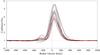 |
Fig. 1 Hα emission line of AB Aur recorded with VEGA from 2010 October to 2013 December. Spectra corresponding to the data set used for the detailed modeling are displayed in red. |
Interferometric observables. We used the standard VEGA pipeline (Mourard et al. 2009) to compute
-
the calibrated squared visibilities
 over a large spectral band centered on Hα (i.e., [640 nm ; 672 nm]);
 -
the differential interferometric visibilities and phases by a cross-spectrum method between two spectral channels [1] and [2]. To reach a sufficient S/N (at least 1 photon per speckle, spectral channel, and single exposure), we consider the spectral band [1] to be as wide as the entire spectral range (i.e., [640 nm ; 672 nm]), and [2] to be as narrow as possible. Sliding the narrow channel [2] across the channel [1] provides a set of differential visibilities and phases as a function of the central wavelength of the channel [2], λi. The effective spectral resolution on these measurements (Rinterf) is always lower than that of the recorded spectrum and depends on the width of [2] (denoted Δλ2). We use Vcont to calibrate the differential interferometric visibilities in the continuum.
The data reduction pipeline produced individual errors for each spectral channel, which only accounts for photon noise. To account for other sources of noise, we adopted conservative errors by considering the highest value between the rms in the continuum and the error computed by the pipeline.
Finally, as AB Aur is a faint target compared to the VEGA limiting magnitude, excellent weather conditions are required to obtain good quality data. As a consequence, only the data recorded on 2010 October 17 and on 2012 September 21 allow us to compute differential visibilities across the Hα line with a spectral sampling of Δλ2 = 0.4 nm, corresponding to an effective spectral resolving power of Rinterf ≃ 1600. Both data sets correspond to a baseline of ~60 m oriented with a PA of about −130°, i.e., in a direction almost parallel to the inner CO disk position angle of 52° ± 1° estimated by Tang et al. (2012). The derived spectra, visibility curves, and differential phases are plotted in Fig. 2.
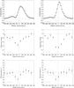 |
Fig. 2 VEGA data recorded on 2010 October 17 (left) and on 2012 September 21 (right). Top: Hα emission line of AB Aur (symbols) and photospheric absorption model (green line). Middle: differential visibilities. Bottom: differential phases. The spectral bin used to compute visibilities and differential phases is represented by the red line in the bottom corner of each panel. |
3. Results
3.1. Spectroscopy
A set of 22 spectra were obtained around the Hα line from 2010 October to 2013 December (Fig. 1). All of our spectra exhibit large wings up to about ±500 km s-1 (see Appendix A). Using the Hα emission line classification of Reipurth et al. (1996), 5 spectra (22%) exhibit a P Cygni profile with blueshifted absorption going below the continuum (type IV-B), 13 (60%) a P Cygni profile with a secondary emission peak in the blue wing less than half of the main emission peak (type III-B), and 4 (18%) spectra are single-peaked (type I). One of the type IV-B spectra shows a very wide blueshifted absorption going out to −500 km s-1 (Fig. A.3). The two spectra for which we have detailed interferometric observations are shown in red in Fig. 1. They show a P Cygni type III-B profile, which is the most frequently observed and appears representative of this class.
A complete study of the spectral variability at Hα is beyond the scope of this paper, but we discuss below some general trends. A strong variability both in the red emission peak (in terms of radial velocity and intensity) and in the blueshifted absorption component is observed, as was already pointed out by several authors (Beskrovnaya et al. 1995; Catala et al. 1999). Our sparse temporal sampling does not allow us to look for periodic behaviors, but we notice a transformation from P Cygni III-B to P Cygni IV-B over a period of a few days only (for instance in 2012, see Fig. A.3). We note that Catala et al. (1999) with a better sampling failed to find a clear period of the Hα line variability. We find no correlation between either the maximum intensity and the radial velocity of the emission peak, or between the radial velocity of the blue and red emission peaks for P Cygni III-B profiles.
3.2. Visibilities and characteristic sizes in the Hα line
Differential visibility and phases. Figure 2 shows the differential visibilities and phases for the Hα line. We clearly observe a visibility drop down to 0.35−0.4 in the core of the line. This visibility drop is asymmetric and the visibility minimum is observed in the blue wing (between −100 km s-1 and −50 km s-1). A visibility decrease to 0.8−0.85 is also observed between −400 km s-1 and −200 km s-1. The phase is null across the line, except between −150 km s-1 and 0 km s-1 where it reaches −30°± 15°. The minimal phase coincides with the minimum of visibility.
Size estimates. We first aim to derive a very rough estimate of the characteristic size of the Hα circumstellar environment by considering a simple model of a Gaussian that includes the inclination of the disk seen by the observer. We assume that the emission is point-symmetric at all wavelengths across the Hα line, and that the stellar photosphere is unresolved at our baseline lengths. The visibilities can be written as  (1)with λi defined in Sect. 2.2 and where the subscript “cs” means circumstellar.
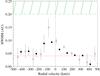 |
Fig. 3 HWHM of the Gaussian disk model for the Hα emitting region of AB Aur observed with VEGA on 2010 October 17 (circles) and on 2012 September 21 (triangles) for i = 23° and PAdisk = 52°. The dotted red line denotes the upper limit of the inner disk truncation radius while the green dash-dotted line denotes the smallest estimate of the dusty disk inner rim. |
The ratio Fcs(λi) /F∗(λi) is null in the continuum. For each wavelength across the line, the ratio is determined from the VEGA spectrum: at each wavelength, we use a photospheric model computed for an effective temperature of 10 000 K (Piétu et al. 2005) and log g = 4 (Prugniel et al. 2007) using PHOENIX models (Husser et al. 2013) so as to estimate the star contribution F∗; we deduce Fcs; and then we integrate the ratio over each spectral bin (whose width equals Δλ2). Assuming i = 23° and PAdisk = 52° (Tang et al. 2012), for each λi we derive the half width at half maximum (HWHM) of the Gaussian disk that best fits the observed differential visibility V(λi). We obtain HWHM of about 0.05 AU in the wings and of 0.10−0.15 AU in the core of the line (Fig. 3). These estimates indicate that the bulk of the Hα emission lies between the magnetospheric truncation radius of the gaseous disk (≤0.04 AU, estimated from Bans & Königl (2012) for equatorial dipolar magnetic field strength less than 1 kG and a disk accretion rate ≥10-8M⊙/yr) and the dusty disk rim radius (0.2−0.5 AU; Tannirkulam et al. 2008).
4. Modeling
The spatial extent of the emission (0.05−0.15 AU) and the asymmetry of the line profile argue against the emission of Hα in magnetospheric accretion columns only. Instead, the P Cygni profiles suggest that it occurs at least partially in a wind. However, as noted in Rousselet-Perraut et al. (2010), a full spherical stellar wind can be excluded as it would produce wider and deeper blueshifted absorption than observed. We thus focus on a scenario in which Hα appears at the base of a disk wind and with a possible contribution of a magnetospheric accretion flow component. This hybrid model is similar to the one developed for classical T Tauri stars by Lima et al. (2010), but has been tailored to the specific parameters of AB Aur. We detail below the components of our model, the radiative transfer tool, and the computation of interferometric predictions.
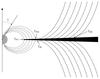 |
Fig. 4 Our composite model (not to scale) including a disk wind and magnetospheric accretion columns. The dotted lines represent the dipolar magnetospheric field lines. The disk (in black) has a constant aspect ratio H/r. The dashed lines are parabolic trajectories that represent the disk wind streamlines. Figure adapted from Lima et al. (2010). |
Stellar parameters adopted for AB Aur.
4.1. Model components
We use the magneto-centrifugally launched disk-wind model described in Lima et al. (2010). We only recall the main properties of the model and the reader can refer to Lima et al. (2010) for the details. The model is based on ideal magneto-hydrodynamics (MHD) with azimuthal symmetry and comprises four different components (Fig. 4) whose parameters are given below.
The star. For AB Aur we adopt the stellar parameters listed in Table 2. We model the photospheric spectrum using a PHOENIX model (Husser et al. 2013) with corresponding parameters.
The accretion disk. We consider a disk with a constant aspect ratio H/r = 0.03, H being the pressure scale height. We assume that the disk is opaque along the vertical direction but does not significantly contribute to the continuum emission. This assumption may no longer be valid below the dust sublimation radius (see Sect. 5.3 for a discussion). We fix PAdisk = 52°, estimated by Tang et al. (2012) for the inner CO disk, which is also compatible with the PA of the thermal radio jet (161°± 7°; Rodríguez et al. 2014) that most likely emerges perpendicularly to the inner disk regions.
The MHD disk-wind model. The model is based on the work by Blandford & Payne (1982) and is described in detail in Lima et al. (2010). It solves the ideal MHD equations considering an axisymmetric magnetic field threading the disk, and assuming a cold flow, where the thermal pressure terms can be neglected. The wind solution is self-similar inside a region limited by the inner and outer wind launching radii rdi and rdo. The disk wind streamlines are described by a self-similar function that can be written as (see Eq. (25) in Lima et al. (2010)) 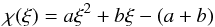 (2)where χ = z/ri, ξ = r/ri, ri is the cylindrical radius where the line crosses the accretion disk mid-plane, and r and z are the usual cylindrical coordinates. The coefficients a and b are related to the initial launching angle (e.g., υ0, the angle between the streamline and disk plane at the launching point) by tanυ0 = (2a + b). The other two variables that define the disk wind solution are κ, the dimensionless ratio between the mass and the magnetic fluxes through the streamline, and λ, the magnetic lever arm. Finally, the density at the base of the disk wind is set by the disk wind mass-loss rate, Ṁloss, and the radial boundaries, rdi and rdo, of the disk ejecting zone.
In this work we adopt inner and outer disk launching radii of rdi = 5 R∗ and rdo = 25 R∗, respectively, from 0.06 to 0.3 AU. The maximum height over the disk zmax over which the solution is computed is set to 30 R∗ (0.35 AU). For a given streamline anchored at a radius r0 in the plane of the disk, the wind solution starts at z(r) = H(r). Not all values of a, b, κ, and λ can produce a physically valid solution for the disk wind. A solution is valid only if the Alfvenic Mach speed increases monotonically along the flux line and it has to cross the critical Alfven point where the poloidal velocity becomes super-Alfvenic. We fix κ = 0.09 and λ = 20−40, which corresponds to a solution very close to the one used by Lima et al. (2010) in the context of T Tauri stars to reproduce Hα profiles. The flow coefficients a and b define the initial disk-wind launching angle υ0. These parameters influence the shape of the line profile, in particular the peak intensity and the depth of the blueshifted absorption. Here we set a = 0.53 and b = −0.1, corresponding to an intermediate disk wind launching angle υ0 = 43.83° and to a solution that – in the context of T Tauri stars – produces type III-B line profiles similar to the ones observed in AB Aur (see Fig. 8 in Lima et al. 2010).
The temperature of the disk wind is assumed to be isothermal as the thermal structure of disk winds is still poorly constrained. Studies of disk winds heated by ambipolar diffusion by Safier (1993) and Garcia et al. (2001) have shown that the wind temperatures quickly reach a plateau at T ≃ 10 000 K after being launched, and slowly change when the wind propagates outward. The remaining free parameters of the disk wind are the inclination i, the wind temperature T, and the mass-loss rate Ṁloss.
The magnetosphere. The model can include an axisymmetric dipolar magnetospheric flow that truncates the accretion disk at a radial distance rmi and extends out to a radial distance rmo. The temperature, density, and velocity profiles in the accretion flow follow the prescriptions given in Lima et al. (2010) and Hartmann et al. (1994). Accretion shocks on the stellar surface are modeled as blackbody rings at the same temperature as the star. None of the calculated profiles includes magnetospheric rotation. The free parameters are rmi and rmo, the accretion rate from the inner disk onto the star Ṁacc, and the minimum and maximum temperatures of the magnetosphere Tmin and Tmax.
Parameters of the disk-wind models for AB Aur.
4.2. Radiative transfer and interferometric observables
To compute the Hα line profiles and synthetic maps, we use a non-LTE model for the hydrogen atom including three levels plus the continuum (Lima et al. 2010). The line source function is calculated with the Sobolev approximation method (Rybicki & Hummer 1978; Hartmann et al. 1994). This method can be applied when the Doppler broadening is much larger than the thermal broadening inside the flow. The emergent flux is calculated using a ray-by-ray method (Muzerolle et al. 2001). Line broadening due to radiative, van der Waals, Stark, and thermal effects are included.
The code provides a spectrum whose infinite spectral resolving power is degraded down to the VEGA spectral resolving power assuming a Gaussian spectral point spread function and intensity maps in different spectral channels with central wavelengths and spectral width as in the VEGA observations (λi, Δλ2). Interferometric observables are computed with a Fourier transform of the intensity maps.
5. Comparison to observations: disk-wind models
We attempt to model both the spectra and the interferometric measurements (differential phases and visibilities) shown in Fig. 2. In a first approach, we do not include a magnetosphere and aim to fit our spectro-interferometric data with a model of a disk wind only as Lima et al. (2010) have shown that the Hα profile is dominated by the disk-wind contribution for mass-loss rates higher than 10-8M⊙/yr. Since the range of parameters to explore is wide and models are computationally expensive, we do not attempt to find a best fit model, but rather investigate a range of solutions with reasonable parameters for inclination, wind temperature, and mass-loss rate. For this purpose, we build three grids of models by considering wind temperatures ranging from 7500 to 8500 K, mass-loss rates varying from 1.7 to 6.8 × 10⁻⁸M⊙/yr (corresponding to fiducial wind densities ρ0 of 1 to 4 × 10⁻¹⁰ g/cm3), and inclinations ranging from 20° to 40° (see Sect. 1).
5.1. Synthetic Hα line profiles
The resulting Hα line profiles and their comparison to the VEGA observations of 2010 are shown in Figs. B.1−B.3. For the range of parameters investigated, a significant fraction of the models produce P Cygni type III-B Hα emission profiles similar to the ones observed in AB Aur. For the two spectra for which we have detailed interferometric observations, the shape of the blueshifted wing, in particular the location and intensity of the blue peak, are best reproduced at low inclinations (20°−30°) and high wind temperatures (8000−8500 K) while the extent of the red wings, in particular for the 2010 spectrum, is best reproduced for intermediate inclinations (30°−40°), high wind temperatures, and high mass-loss rates.
The best agreement to the relative shape of the line profile measured in 2010 is obtained for a wind mass-loss rate of 6.8 × 10⁻⁸M⊙/yr, a wind temperature of 8500 K, and a system inclination of 30°. However, the line-to-continuum ratio exceeds the observed value by a factor ≃7. This issue remains even when the mass-loss rate is decreased to 1.7 × 10⁻⁸M⊙/yr, as the line-to-continuum ratio is still 2.5 to 4 times higher than the observed value. The line-to-continuum ratio is lower when the wind mass-loss rate or the isothermal disk wind temperature decreases, or alternatively, when the inclination increases. A good agreement with the observed line-to-continuum ratio is obtained in our grid for a mass-loss rate of 1.7 × 10⁻⁸M⊙/yr, an inclination of 30°, and an isothermal disk wind temperature of 7500 K, but with these parameters the width and the shape of the line profile is not well reproduced, in particular the extent of the red wing and the position and depth of the blue-shifted absorption.
We select two representative disk wind solutions, one with a line-to-continuum ratio similar to that of the observations (model M1), and one with a better agreement of the line width but a line-to-continuum ratio that is twice as high as the observations (model M2). The parameters of both models are given in Table 3.
5.2. Modeling the spectro-interferometric data
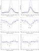 |
Fig. 5 Modeling of the VEGA observations on 2010 October 17 (left) and 2012 September 21 (right). Top: observed (black circles) and modeled spectra for all disk-wind models (M1: dashed line; M2: dotted line; M3: solid line). The dash-dotted red line indicates the contribution of the magnetosphere to the profile for M3. Middle: same for differential visibilities. Bottom: same for differential phases. The spectral bin is represented by the red line in the bottom corner of each panel. |
The modeled differential observables across Hα are compared for both observations in Fig. 5. Both models (M1 and M2) produce a visibility drop on the order of that observed in the core of the line. A deeper and larger visibility drop is obtained for model M2 whose line-to-continuum ratio is higher by a factor 2.5 compared to model M1 and the observations. For both models, the minimal visibility is reached in the red wing of the line at ~100 km s-1. Considering the spectral bin used to compute the interferometric observables, model M2 matches the visibility curve well in the 2012 data. For the observations of 2010, model M2 also matches the blue part of the visibility curve, but leads to a visibility drop too deep in the red wing of the line. For the 2010 data, the observed visibility in the core of the line is better reproduced by model M1. With regard to the phase, both models predict a slightly asymmetric S-shaped signals, but they fail to reproduce the minimum phase signal of about −30° ± 15° in the blue wing of the line.
Our analysis thus demonstrates that a Blandford & Payne MHD disk wind solution arising from the inner sub-AU regions of the accretion disk with mass flux higher than 10-8M⊙/yr and seen at moderate inclinations (30°) produces Hα lines with similar emission profiles and size scales as observed in AB Aur. However, with the disk wind solution adopted, such type III-B profiles with prominent redshifted wings require either high wind temperatures or mass-flux, resulting in higher line-to-continuum ratios than observed in AB Aur. In addition, the differential phase amplitudes are not well reproduced. The predicted phase amplitude is too small, which might be related to our isothermal hypothesis that puts weight on the basis of the wind. Differential phases and visibilities depend critically on the line-to-continuum ratio. Improving the agreement with observations therefore first requires a better match to this parameter. We discuss below possible origins for the observed discrepancies and suggestions to improve agreement with observations.
5.3. Improving the line-to-continuum ratio
Exploring different disk wind solutions, leading to different acceleration and collimation properties than adopted in this work, may help improve the agreement with the AB Aur observations. Indeed, the study conducted by Kurosawa et al. (2006) in the context of lower mass T Tauri stars, showed that the line profile, in particular the depth and location of the blueshifted absorption component, but also the line-to-continuum ratio, are very sensitive to the wind acceleration rate along the streamline parametrized in their study with the β parameter (see their Fig. 6). A detailed comparison with our model predictions is difficult, however, as both the MHD disk wind solution and the photospheric contributions are significantly different.
One way to decrease the line-to-continuum ratio in the models would be to add a continuum contribution in addition to the photospheric one. However, both the inner gaseous disk and the magnetosphere are not expected to have significant optical emissivities for accretion rates of about 10-7M⊙/yr (Muzerolle et al. 2004; Natta et al. 2001). Natta et al. (2001) compute inner gaseous disk model predictions tailored to AB Aur. Disk emission shortward of 1 μm is negligible unless the inner disk extends to the stellar surface (see their Fig. 6). Even in this case, the expected contribution is on the order of the photospheric contribution, therefore reducing the line-to-continuum ratio by a factor 2 at most.
The presence of dust in the disk wind would be another possible way to reduce the line-to-continuum ratio. Dust lifted off the plane of the disk along streamlines anchored at radii beyond the dust sublimation front could partially occult the inner disk wind Hα emission. Evidence for dusty disk winds has been recently presented in the Herbig Ae star HD 163296 (Ellerbroek et al. 2014). Finally, if the inner gaseous disk is vertically partially optically thin, we may see part of the receding flow through the gaseous inner disk, which may increase the redshifted wing emission significantly. This effect has been invoked to reproduce the detection of spatial offsets in the Paβ line on scales much smaller than the disk itself (Whelan et al. 2004).
In any of these scenarios, consistent radiative transfer taking into account these additional components/effects would be required to compute accurate Hα line predictions, which is beyond the scope of this paper.
6. Comparison to observations: disk wind plus magnetospheric accretion flow
In this section we investigate whether adding the contribution of an inner magnetospheric flow could improve the agreement between models and observations. Chemical peculiarities of the λ Boo type (Folsom et al. 2012) and X-ray emission (Hamidouche et al. 2008) are both detected in AB Aur, suggesting a significant amount of magnetic activity. Although signatures of a stellar magnetic field have not been detected so far on AB Aur, we cannot fully exclude the presence of a magnetosphere on this star. Indeed Alecian et al. (2013) have clearly shown that the average Stokes I profile is dominated by a strong circumstellar emission component in AB Aur (see their Fig. 8). Therefore, no reliable constraint on the stellar magnetic field can be derived from spectro-polarimetric measurements.
For an accretion rate lower than 2 × 10⁻⁷M⊙/yr (i.e., the upper limit of accretion rate estimates in AB Aur), we expect the accretion disk to be truncated at r< 2 R∗ for B< 1 kG (Bans & Königl 2012), thus suggesting a close and compact magnetosphere. We therefore set the inner and outer radii of the magnetospheric flow at 1.4 and 2 R∗, respectively. We combine this compact magnetosphere with a disk wind solution similar to the one adopted before. We do not attempt to find the best fit solution, but we allow for a small variation of the parameters of the magnetosphere (the accretion rate and the temperature) and the disk wind to find a reasonable agreement with both the line shape and the line-to-continuum ratio.
We list in Table 3 the parameters of our best hybrid model (model M3) and show its predicted spectrum, visibilities, and differential phases in Fig. 5. The best agreement with observations is found for an accretion rate of 2.6 × 10⁻⁷M⊙/yr and a hot magnetospheric temperature (9700−13 000 K). The disk wind solution is slightly cooler and more massive than in the models M1 and M2. In addition, we could not find a significant improvement, with respect to the disk wind solution alone, when the system inclination was kept at values as low as those of models M1 and M2. A good agreement was found by allowing the inclination to be as high as 50°. In this model, the disk wind component dominates the emission at Hα, consistent with the prediction by Lima et al. (2010) for a disk wind mass-loss rate ≥ 10-8M⊙/yr. However, the addition of a magnetospheric component results in both a line shape and line-to-continuum ratio closer to the observed values (Fig. 5 for an example). Indeed, the magnetospheric component contributes more to the wings of the profile allowing us to use a disk wind solution with lower temperature and higher inclination (resulting in a lower line-to-continuum ratio), while keeping good agreement with the shape of the blue wing.
Model M3 also reproduces reasonably well both the differential visibility and phase across Hα, which was not the case for M1 and M2. Such hybrid solutions, however, result in more compact intensity maps, and the observed visibility drop across Hα is thus not perfectly reproduced. For a line-to-continuum ratio close to 5, the visibility drop never goes below 0.6 in the core of the line because of a significant contribution from the compact magnetosphere (Fig. 5). On the other hand, extending the size of the magnetosphere will increase its contribution to the line profile and hence produce even higher visibilities, unless unrealistic magnetospheric outer radii are used (>10 R∗). The high inclination found for model M3 is intriguing, but at the same time cannot be fully excluded by the current observational constraints. The range of inclination quoted in the literature for AB Aur is wide (from 20° to >50°; see Sect. 1) and variation of disk inclination with distance to the source has been already reported on larger scales (Tang et al. 2012). The adopted mass accretion and mass-loss rates for model M3 are 2.6 × 10⁻⁷M⊙/yr and 4.7 × 10⁻⁸M⊙/yr, which results in a ratio of ejection to accretion rate of 0.18. This ratio is higher than the average value of 0.1 found from resolved observations of large-scale jets, but is still compatible with expectations from magneto-centrifugal ejection models (Ferreira et al. 2006).
The solution presented in this paper is not a best fit and a full exploration of the model parameter space is required before a firm conclusion can be reached. However, it is striking that such a hybrid solution, very similar to the one proposed in the context of classical T Tauri stars by Lima et al. (2010) and with reasonable parameters for AB Aur, matches quite satisfactorily both the observed spectra and interferometric measurements at Hα. These results also go in the same direction as the recent spectro-interferometric studies of Herbig stars conducted on the HI Brγ emission line by Weigelt et al. (2011), Garcia Lopez et al. (2015), Caratti o Garatti et al. (2015), and Kurosawa et al. (2016). All these studies conclude that the best agreement with observations is found using a model combining a small magnetosphere and a compact disk wind. Kurosawa et al. (2016) tentatively find a positive correlation between the disk-wind inner launching radius and the luminosity of the central star. The inner launching radius derived for our best disk wind solution in AB Aur (rdi = 5 R∗ = 0.06 AU) follows the general trend found by Kurosawa et al. (2006) of a more compact disk wind for lower luminosity sources. All these new results therefore confirm that mass-loss processes, powered by accretion, play a major role in the formation of the HI lines in young stars.
7. Conclusion
We have presented results from multi-epoch spectro-interferometric observations (22) across the Hα line of the Herbig Ae star AB Aur conducted with the VEGA interferometer. For two epochs we reconstruct differential visibilities and phases across Hα with more than ten velocity resolution elements. These are the first interferometric measurements at Hα of a young accreting star with such a spectral resolution.
The variability in the Hα spectroscopic profiles is similar to previous observations. The two spectra for which we have detailed interferometric observations show a P Cygni type III-B profile (a P Cygni profile with a secondary emission peak in the blue wing less than half of the main emission peak), which is by far the most frequently observed in our sample (60%).
Our spectro-interferometric observations clearly resolve the Hα formation region of the Herbig Ae star AB Aur at both epochs. No significant variation in the interferometric measurements is observed. Using a Gaussian model we derive a half width at half maximum of 0.05−0.15 AU for the core of the line emission, implying size scales intermediate between the inner disk truncation radius (<0.04 AU) and the inner rim of the dust disk (>0.2 AU). We also detect a clear asymmetric phase signal with a minimum of −30° ± 15°. These observations suggest that the bulk of the Hα line cannot be formed in a magnetospheric accretion flow alone, and favor a disk wind origin.
To interpret these observations we compute 2D radiative transfer at Hα in a model combining a magneto-centrifugal Blandford & Payne disk wind solution with an axisymmetric magnetospheric accretion flow and with the parameters tailored to the AB Aur system. Comparison with the observations shows general agreement with predictions from disk winds arising from the inner radii of the gaseous disk (r = 5−25 R∗ = 0.06−0.3 AU). Hα is formed in the very inner accelerating regions of the wind at a few scale heights above the disk. Adding a compact magnetospheric component allows us to better reproduce the line-to-continuum ratio and the differential phase signal across the line, but the line profile remains dominated by the disk wind component. Our best model is obtained for a high inclination of the magnetosphere and inner disk (i = 50°) and implies an ejection-to-accretion rate ratio of ≃0.2, consistent with magneto-centrifugal launching processes. Similar models have recently been proposed to account for spectro-interferometric observations at high spectral resolution in the HI Brγ line of four Herbig stars. These new results all suggest that mass-loss processes, likely powered by accretion, play a major role in the formation of the HI lines in young stars.
Finally, our analysis is focused on two profiles, representative of the type III-B profiles observed in AB Aur. However, a clear profile variability is observed. In our disk-wind models, we never get type IV-B profiles with wide blueshifted absorptions below the continuum; this profile represents 22% of our observed profiles. These wide blueshifted absorptions could trace an additional inner wide-angle wind component of stellar or magnetospheric origin. This component may also be responsible for the variation in inner disk wind streamlines, inducing additional profile variability. The origin of the short timescale variability of the Hα profile is still matter of debate, and continued monitoring combined with dedicated modeling is also required.
Acknowledgments
We wish to pay tribute to Olivier Chesneau, who passed away in 2014 May, for all the fruitful discussions and the relevant advice about this research program. G.H.R.A. Lima acknowledges financial support from CAPES and FAPEMIG. VEGA is supported by French programs for stellar physics and high angular resolution, PNPS and ASHRA, by the Nice Observatory, and by the Lagrange Department. This work is based upon observations obtained with the Georgia State University Center for High Angular Resolution Astronomy Array at Mount Wilson Observatory. The CHARA Array is supported by the National Science Foundation under Grant No. AST-1211929. Institutional support has been provided from the GSU College of Arts and Sciences and the GSU Office of the Vice President for Research and Economic Development. We acknowledge financial support from the Programme National de Physique Stellaire (PNPS) of CNRS/INSU, France. This research has made use of the SearchCal service of the Jean-Marie Mariotti Center, and of CDS Astronomical Databases SIMBAD and VIZIER. We thank Dr. J. Aufdenberg for providing photospheric Hα models.
References
- Alecian, E., Wade, G. A., Catala, C., et al. 2013, MNRAS, 429, 1001 [NASA ADS] [CrossRef] [Google Scholar]
- Bans, A., & Königl, A. 2012, ApJ, 758, 100 [NASA ADS] [CrossRef] [Google Scholar]
- Benisty, M., Malbet, F., Dougados, C., et al. 2010, A&A, 517, L3 [NASA ADS] [CrossRef] [EDP Sciences] [Google Scholar]
- Beskrovnaya, N. G., Pogodin, M. A., Najdenov, I. D., & Romanyuk, I. I. 1995, A&A, 298, 585 [NASA ADS] [Google Scholar]
- Blandford, R. D., & Payne, D. G. 1982, MNRAS, 199, 883 [NASA ADS] [CrossRef] [Google Scholar]
- Boehm, T., & Catala, C. 1995, A&A, 301, 155 [NASA ADS] [Google Scholar]
- Bohm, T., & Catala, C. 1993, A&AS, 101, 629 [NASA ADS] [Google Scholar]
- Caratti o Garatti, A., Tambovtseva, L. V., Garcia Lopez, R., et al. 2015, A&A, 582, A44 [NASA ADS] [CrossRef] [EDP Sciences] [Google Scholar]
- Catala, C., & Kunasz, P. B. 1987, A&A, 174, 158 [NASA ADS] [Google Scholar]
- Catala, C., Donati, J. F., Böhm, T., et al. 1999, A&A, 345, 884 [NASA ADS] [Google Scholar]
- DeWarf, L. E., Sepinsky, J. F., Guinan, E. F., Ribas, I., & Nadalin, I. 2003, ApJ, 590, 357 [NASA ADS] [CrossRef] [EDP Sciences] [Google Scholar]
- Donehew, B., & Brittain, S. 2011, AJ, 141, 46 [NASA ADS] [CrossRef] [Google Scholar]
- Eisner, J. A., Hillenbrand, L. A., & Stone, J. M. 2014, MNRAS, 443, 1916 [NASA ADS] [CrossRef] [Google Scholar]
- Ellerbroek, L. E., Podio, L., Dougados, C., et al. 2014, A&A, 563, A87 [NASA ADS] [CrossRef] [EDP Sciences] [Google Scholar]
- Ferreira, J., Dougados, C., & Cabrit, S. 2006, A&A, 453, 785 [NASA ADS] [CrossRef] [EDP Sciences] [Google Scholar]
- Folsom, C. P., Bagnulo, S., Wade, G. A., et al. 2012, MNRAS, 422, 2072 [NASA ADS] [CrossRef] [MathSciNet] [Google Scholar]
- Fukagawa, M., Hayashi, M., Tamura, M., et al. 2004, ApJ, 605, L53 [NASA ADS] [CrossRef] [Google Scholar]
- Garcia, P. J. V., Ferreira, J., Cabrit, S., & Binette, L. 2001, A&A, 377, 589 [NASA ADS] [CrossRef] [EDP Sciences] [Google Scholar]
- Garcia Lopez, R., Natta, A., Testi, L., & Habart, E. 2006, A&A, 459, 837 [NASA ADS] [CrossRef] [EDP Sciences] [Google Scholar]
- Garcia Lopez, R., Tambovtseva, L. V., Schertl, D., et al. 2015, A&A, 576, A84 [NASA ADS] [CrossRef] [EDP Sciences] [Google Scholar]
- Garrison, Jr., L. M. 1978, ApJ, 224, 535 [NASA ADS] [CrossRef] [Google Scholar]
- Grady, C. A., Pérez, M. R., Bjorkman, K. S., & Massa, D. 1999a, ApJ, 511, 925 [NASA ADS] [CrossRef] [Google Scholar]
- Grady, C. A., Woodgate, B., Bruhweiler, F. C., et al. 1999b, ApJ, 523, L151 [NASA ADS] [CrossRef] [Google Scholar]
- Hamidouche, M., Wang, S., & Looney, L. W. 2008, AJ, 135, 1474 [NASA ADS] [CrossRef] [Google Scholar]
- Hartmann, L., Hewett, R., & Calvet, N. 1994, ApJ, 426, 669 [NASA ADS] [CrossRef] [Google Scholar]
- Hashimoto, J., Tamura, M., Muto, T., et al. 2011, ApJ, 729, L17 [NASA ADS] [CrossRef] [Google Scholar]
- Husser, T.-O., Wende-von Berg, S., Dreizler, S., et al. 2013, A&A, 553, A6 [NASA ADS] [CrossRef] [EDP Sciences] [Google Scholar]
- Kraus, S., Hofmann, K.-H., Benisty, M., et al. 2008, A&A, 489, 1157 [NASA ADS] [CrossRef] [EDP Sciences] [Google Scholar]
- Kurosawa, R., Harries, T. J., & Symington, N. H. 2006, MNRAS, 370, 580 [NASA ADS] [CrossRef] [Google Scholar]
- Kurosawa, R., Kreplin, A., Weigelt, G., et al. 2016, MNRAS, 457, 2236 [NASA ADS] [CrossRef] [Google Scholar]
- Lafrasse, S., Mella, G., Bonneau, D., et al. 2010, VizieR Online Data Catalog: II/300 [Google Scholar]
- Lima, G. H. R. A., Alencar, S. H. P., Calvet, N., Hartmann, L., & Muzerolle, J. 2010, A&A, 522, A104 [NASA ADS] [CrossRef] [EDP Sciences] [Google Scholar]
- Liu, W. M., Hinz, P. M., Meyer, M. R., et al. 2007, ApJ, 658, 1164 [NASA ADS] [CrossRef] [Google Scholar]
- Mendigutía, I., de Wit, W. J., Oudmaijer, R. D., et al. 2015, MNRAS, 453, 2126 [NASA ADS] [CrossRef] [Google Scholar]
- Mourard, D., Clausse, J. M., Marcotto, A., et al. 2009, A&A, 508, 1073 [NASA ADS] [CrossRef] [EDP Sciences] [Google Scholar]
- Muzerolle, J., Calvet, N., & Hartmann, L. 2001, ApJ, 550, 944 [NASA ADS] [CrossRef] [Google Scholar]
- Muzerolle, J., D’Alessio, P., Calvet, N., & Hartmann, L. 2004, ApJ, 617, 406 [NASA ADS] [CrossRef] [Google Scholar]
- Natta, A., Prusti, T., Neri, R., et al. 2001, A&A, 371, 186 [NASA ADS] [CrossRef] [EDP Sciences] [Google Scholar]
- Perrin, M. D., Schneider, G., Duchene, G., et al. 2009, ApJ, 707, L132 [NASA ADS] [CrossRef] [Google Scholar]
- Piétu, V., Guilloteau, S., & Dutrey, A. 2005, A&A, 443, 945 [NASA ADS] [CrossRef] [EDP Sciences] [Google Scholar]
- Prugniel, P., Soubiran, C., Koleva, M., & Le Borgne, D. 2007, ArXiv e-prints [arXiv:0703658] [Google Scholar]
- Ray, T. P. 2007, in Star-Disk Interaction in Young Stars, eds. J. Bouvier, & I. Appenzeller, IAU Symp., 243, 183 [Google Scholar]
- Reipurth, B., Pedrosa, A., & Lago, M. T. V. T. 1996, A&AS, 120, 229 [NASA ADS] [CrossRef] [EDP Sciences] [Google Scholar]
- Rodríguez, L. F., Zapata, L. A., Dzib, S. A., et al. 2014, ApJ, 793, L21 [NASA ADS] [CrossRef] [Google Scholar]
- Rousselet-Perraut, K., Benisty, M., Mourard, D., et al. 2010, A&A, 516, L1 [NASA ADS] [CrossRef] [EDP Sciences] [Google Scholar]
- Rybicki, G. B., & Hummer, D. G. 1978, ApJ, 219, 654 [NASA ADS] [CrossRef] [Google Scholar]
- Safier, P. N. 1993, ApJ, 408, 115 [NASA ADS] [CrossRef] [Google Scholar]
- Sturmann, J., Ten Brummelaar, T., Sturmann, L., & McAlister, H. A. 2010, SPIE Conf. Ser., 7734, 773445 [Google Scholar]
- Tang, Y.-W., Guilloteau, S., Piétu, V., et al. 2012, A&A, 547, A84 [NASA ADS] [CrossRef] [EDP Sciences] [Google Scholar]
- Tannirkulam, A., Monnier, J. D., Harries, T. J., et al. 2008, ApJ, 689, 513 [NASA ADS] [CrossRef] [Google Scholar]
- ten Brummelaar, T. A., McAlister, H. A., Ridgway, S. T., et al. 2005, ApJ, 628, 453 [NASA ADS] [CrossRef] [Google Scholar]
- van den Ancker, M. E., Volp, A. W., Perez, M. R., & de Winter, D. 1999, Information Bulletin on Variable Stars, 4704, 1 [Google Scholar]
- van Leeuwen, F. 2007, A&A, 474, 653 [NASA ADS] [CrossRef] [EDP Sciences] [Google Scholar]
- Wade, G. A., Bagnulo, S., Drouin, D., Landstreet, J. D., & Monin, D. 2007, MNRAS, 376, 1145 [NASA ADS] [CrossRef] [MathSciNet] [Google Scholar]
- Weigelt, G., Grinin, V. P., Groh, J. H., et al. 2011, A&A, 527, A103 [NASA ADS] [CrossRef] [EDP Sciences] [Google Scholar]
- Whelan, E. T., Ray, T. P., & Davis, C. J. 2004, A&A, 417, 247 [NASA ADS] [CrossRef] [EDP Sciences] [Google Scholar]
Appendix A: All VEGA spectra of AB Aur
All the spectra recorded with VEGA around the Hα line with a spectral resolving power of about 5000 are displayed in Figs. A.1, A.2, and A.3.
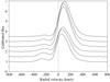 |
Fig. A.1 Hα line of AB Aur recorded with VEGA in 2010. Spectra are plotted in chronological order from bottom to top. They are shifted by 0.5 along the y axis for clarity. |
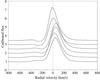 |
Fig. A.2 Same as Fig. A.1. for 2011. |
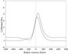 |
Fig. A.3 Same as Fig. A.1. for 2012. |
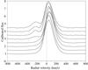 |
Fig. A.4 Same as Fig. A.1. for 2013. |
Appendix B: Grids of models of the AB Aur disk wind only
All the grids of models that we computed for the disk wind only are displayed in Figs. B.1–B.3.
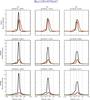 |
Fig. B.1 Grid of models of AB Aur disk wind for different effective temperatures, for different inclinations, and for a mass-loss rate of 1.7 × 10⁻⁸M⊙/yr: modeled spectrum at the VEGA spectral resolution (black), observed spectrum (red), and modeled spectrum rescaled to have the same maximum intensity as the observed spectrum (green). |
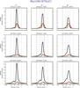 |
Fig. B.2 Grid of models of AB Aur disk wind for different effective temperatures, for different inclinations, and for a mass-loss rate of 3.4 × 10⁻⁸M⊙/yr. The color code is the same as in Fig. B.1. |
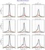 |
Fig. B.3 Grid of models of AB Aur disk wind for different effective temperatures, for different inclinations, and for a mass-loss rate of 6.8 × 10⁻⁸M⊙/yr. The color code is the same as in Fig. B.1. |
All Tables
All Figures
|
Fig. 1 Hα emission line of AB Aur recorded with VEGA from 2010 October to 2013 December. Spectra corresponding to the data set used for the detailed modeling are displayed in red. |
| In the text | |
|
Fig. 2 VEGA data recorded on 2010 October 17 (left) and on 2012 September 21 (right). Top: Hα emission line of AB Aur (symbols) and photospheric absorption model (green line). Middle: differential visibilities. Bottom: differential phases. The spectral bin used to compute visibilities and differential phases is represented by the red line in the bottom corner of each panel. |
| In the text | |
|
Fig. 3 HWHM of the Gaussian disk model for the Hα emitting region of AB Aur observed with VEGA on 2010 October 17 (circles) and on 2012 September 21 (triangles) for i = 23° and PAdisk = 52°. The dotted red line denotes the upper limit of the inner disk truncation radius while the green dash-dotted line denotes the smallest estimate of the dusty disk inner rim. |
| In the text | |
|
Fig. 4 Our composite model (not to scale) including a disk wind and magnetospheric accretion columns. The dotted lines represent the dipolar magnetospheric field lines. The disk (in black) has a constant aspect ratio H/r. The dashed lines are parabolic trajectories that represent the disk wind streamlines. Figure adapted from Lima et al. (2010). |
| In the text | |
|
Fig. 5 Modeling of the VEGA observations on 2010 October 17 (left) and 2012 September 21 (right). Top: observed (black circles) and modeled spectra for all disk-wind models (M1: dashed line; M2: dotted line; M3: solid line). The dash-dotted red line indicates the contribution of the magnetosphere to the profile for M3. Middle: same for differential visibilities. Bottom: same for differential phases. The spectral bin is represented by the red line in the bottom corner of each panel. |
| In the text | |
|
Fig. A.1 Hα line of AB Aur recorded with VEGA in 2010. Spectra are plotted in chronological order from bottom to top. They are shifted by 0.5 along the y axis for clarity. |
| In the text | |
|
Fig. A.2 Same as Fig. A.1. for 2011. |
| In the text | |
|
Fig. A.3 Same as Fig. A.1. for 2012. |
| In the text | |
|
Fig. A.4 Same as Fig. A.1. for 2013. |
| In the text | |
|
Fig. B.1 Grid of models of AB Aur disk wind for different effective temperatures, for different inclinations, and for a mass-loss rate of 1.7 × 10⁻⁸M⊙/yr: modeled spectrum at the VEGA spectral resolution (black), observed spectrum (red), and modeled spectrum rescaled to have the same maximum intensity as the observed spectrum (green). |
| In the text | |
|
Fig. B.2 Grid of models of AB Aur disk wind for different effective temperatures, for different inclinations, and for a mass-loss rate of 3.4 × 10⁻⁸M⊙/yr. The color code is the same as in Fig. B.1. |
| In the text | |
|
Fig. B.3 Grid of models of AB Aur disk wind for different effective temperatures, for different inclinations, and for a mass-loss rate of 6.8 × 10⁻⁸M⊙/yr. The color code is the same as in Fig. B.1. |
| In the text | |
Current usage metrics show cumulative count of Article Views (full-text article views including HTML views, PDF and ePub downloads, according to the available data) and Abstracts Views on Vision4Press platform.
Data correspond to usage on the plateform after 2015. The current usage metrics is available 48-96 hours after online publication and is updated daily on week days.
Initial download of the metrics may take a while.