© ESO, 2016

1. Introduction

Observations in the solar neighborhood, on Earth, in binary pulsar systems, and now of gravitational waves (LIGO Collaboration & Virgo Collaboration 2016) constrain possible deviations from general relativity (GR) with extraordinary precision (Will 2014). This presents a formidable challenge to alternative theories of gravity, such as those being developed as a potential explanation of cosmic acceleration (Clifton et al. 2012; Joyce et al. 2015; Bull et al. 2016); the slightest disagreement with GR on the relevant scales can invalidate a given theory instantly.

With the partial exception of gravitational waves, which propagate over cosmological distances, the subjects of all of these tests are astrophysical systems that reside in dense galactic environments. Here, conditions are far from the cosmological average: the matter density, curvature, and gravitational potential may differ from the background by several orders of magnitude (Baker et al. 2015). One way of evading the stringent small-scale constraints while still allowing non-trivial deviations from GR on large scales is therefore to screen modifications to GR in certain environments. Several such screening mechanisms have been proposed, but all fall into one of three categories: Chameleon, K-mouflage, or Vainshtein screening (Brax 2013; Brax & Davis 2015). In each case, deviations from GR are suppressed according to either the value of the scalar field or its derivatives, which vary depending on environmental factors such as ambient matter density or proximity to massive objects.

Screening mechanisms are a relatively generic prediction of viable modified gravity (MG) theories (Brax et al. 2012), and so detecting one at work would be a powerful indicator of beyond-GR physics. Observational tests of screening necessarily focus on the transition between the fully screened and unscreened regimes, where differences from GR phenomenology are expected to be most pronounced. For most viable cosmological theories, this transition is expected to occur at the outskirts of dark matter halos, where the matter density and gravitational potential begin to to approach their background values. A number of studies have looked for signatures of modified gravity in this region, for example through differences in halo or galaxy clustering statistics (e.g., Shirata et al. 2005; Davis et al. 2012; Oyaizu et al. 2008; Schmidt et al. 2009; Barreira et al. 2013; Wyman et al. 2013; Li et al. 2013; Zhao 2014; Clifton et al. 2005; Lombriser et al. 2015), or the density, velocity, and potential profiles of individual halos (e.g., Martino & Sheth 2009; Lombriser et al. 2012; Clampitt et al. 2013; Hellwing et al. 2013; Gronke et al. 2014, 2015a; Stark et al. 2016).

In this paper, we study the effect of modifications to GR on pairwise peculiar velocity statistics (Davis & Peebles 1977), a relatively model-independent class of observables (Ferreira et al. 1999) that probe scales that are well-matched to the expected screening transition. Some of these statistics were recently found to exhibit strong deviations from their GR behavior on quasi-linear and non-linear scales in simulations of f(R) and Galileon theories (Hellwing et al. 2014).

Here, we use similar simulations of f(R) and symmetron theories to investigate the environmental dependence of the deviations. We find that a clear, theory-dependent signature of screening can be observed when the ambient matter density, smoothed on scales on the order of the inter-halo separation, is chosen as the proxy for environment. Other proxies also have interesting theory-dependent behaviors, but are harder to interpret. We also clarify the relationship between theoretical pairwise velocity statistics and observable (line-of-sight) quantities, and propose a new estimator for the pairwise velocity dispersion σ_∥ (sometimes called σ₁₂). The result of our study is an observable that is sensitive to the theory-dependent properties of screening mechanisms, and a set of predictions for what those signatures should look like in f(R) and symmetron gravity.

The paper is organized as follows. In Sect. 2 we give an overview of the MG theories and simulations that we used, and outline predictions for screening effects based on previous work. In Sect. 3 we define several relevant velocity statistics, and clarify their relationship with observables. Then, in Sect. 4, we define two ways of measuring halo environment and briefly compare them. Finally, we present results from the simulations in Sect. 5, and we conclude in Sect. 6.

2. Modified gravity simulations

In this section, we describe the suite of N-body simulations used in this study. In addition to a reference GR/ΛCDM simulation, we used three simulations of f(R) modified-gravity models (Hu & Sawicki 2007) and four simulations of symmetron modified-gravity models (Hinterbichler et al. 2011). Both types of MG model screen the fifth force in high-density environments by way of a chameleon-like screening that depends on the value of an additional scalar field. In what follows, we provide a brief overview of the particular modified-gravity models that were used, and describe the basic properties of the simulations. More details about the simulations can be found in Llinares et al. (2014).

2.1. f(R) gravity

A simple way of modifying GR is to replace the Ricci scalar, R, in the Einstein-Hilbert action with a more general function f(R),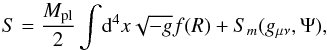$\mathit{S}\mathrm{=}\frac{{\mathit{M}}_{\mathrm{pl}}}{\mathrm{2}}\mathrm{\int }{\mathrm{d}}^{\mathrm{4}}\mathit{x}\sqrt{\mathrm{-}\mathit{g}}\mathit{f}\mathrm{\left(}\mathit{R}\mathrm{\right)}\mathrm{+}{\mathit{S}}_{\mathit{m}}\mathrm{\left(}{\mathit{g}}_{\mathit{\mu \nu }}\mathit{,}\mathrm{\Psi }\mathrm{\right)}\mathit{,}$(1)where M_pl = (8πG)^{− 1/2}, G is the bare gravitational constant, g is the determinant of the spacetime metric g_μν, and S_m is the action for matter fields Ψ. By applying an appropriate conformal transformation, these models can be written as an effective scalar field theory for any choice of the function f(R) (Clifton et al. 2012). The resulting scalar field, f_R ≡ df/ dR, gives rise to a so-called fifth force, 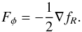${\mathit{F}}_{\mathit{\phi }}\mathrm{=}\mathrm{-}\frac{\mathrm{1}}{\mathrm{2}}\mathrm{\nabla }{\mathit{f}}_{\mathit{R}}\mathit{.}$(2)Screening of the fifth force (e.g., to satisfy solar system constraints) is achieved using the chameleon mechanism. The scalar field f_R propagates in an effective potential,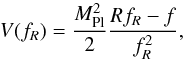$\mathit{V}\mathrm{\left(}{\mathit{f}}_{\mathit{R}}\mathrm{\right)}\mathrm{=}\frac{{\mathit{M}}_{\mathrm{Pl}}^{\mathrm{2}}}{\mathrm{2}}\frac{\mathit{R}{\mathit{f}}_{\mathit{R}}\mathrm{-}\mathit{f}}{{\mathit{f}}_{\mathit{R}}^{\mathrm{2}}}\mathit{,}$(3)with a density-dependent effective mass (Amendola & Tsujikawa 2010). In high-density environments, the mass becomes high and the effective potential steepens, stopping the field from propagating freely, and sending F_φ → 0.

Models are specified by choosing a particular form for f(R). A commonly used parametrization introduces a single extra parameter f_R0, the value of the scalar field at the present epoch (Hu & Sawicki 2007). This parameter controls the degree to which the model deviates from GR, that is, f_R0 → 0 is the GR limit. The three f(R) models for which we have simulations differ only by the field value: f_R0 = { 10^-6,10^-5,10^-4 } (in order of weakest to strongest deviation from GR). We note that these models are disfavored by current data (e.g., Jain et al. 2013; Planck Collaboration XIV 2016), but nevertheless remain useful for the purposes of illustration.

2.2. Symmetron gravity

Symmetron gravity explicitly introduces a new scalar field into the gravitational action (Pietroni 2005; Hinterbichler & Khoury 2010; Hinterbichler et al. 2011), $\mathit{S}\mathrm{=}\mathrm{\int }{\mathrm{d}}^{\mathrm{4}}\mathit{x}\sqrt{\mathrm{-}\mathit{g}}\left[\frac{{\mathit{M}}_{\mathrm{pl}}}{\mathrm{2}}\mathit{R}\mathrm{-}\frac{\mathrm{1}}{\mathrm{2}}{\mathit{g}}^{\mathit{ab}}{\mathit{\partial }}_{\mathit{a}}\mathit{\phi }{\mathit{\partial }}_{\mathit{b}}\mathit{\phi }\mathrm{-}\mathit{V}\mathrm{\left(}\mathit{\phi }\mathrm{\right)}\right]\mathrm{+}{\mathit{S}}_{\mathit{m}}\mathrm{\left(}\begin{array}{c}\mathrm{˜}\\ {\mathit{g}}_{\mathit{\mu \nu }}\end{array}\mathit{,}\mathrm{\Psi }\mathrm{\right)}\mathit{,}$(4)which means that the Einstein-Hilbert term has been supplemented by a kinetic term and potential V for the scalar field φ. A key element of symmetron theories is the choice of a symmetry breaking form for the effective potential, such as (Hinterbichler et al. 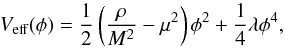2011) ${\mathit{V}}_{\mathrm{eff}}\mathrm{\left(}\mathit{\phi }\mathrm{\right)}\mathrm{=}\frac{\mathrm{1}}{\mathrm{2}}\left(\frac{\mathit{\rho }}{{\mathit{M}}^{\mathrm{2}}}\mathrm{-}{\mathit{\mu }}^{\mathrm{2}}\right){\mathit{\phi }}^{\mathrm{2}}\mathrm{+}\frac{\mathrm{1}}{\mathrm{4}}\mathit{\lambda }{\mathit{\phi }}^{\mathrm{4}}\mathit{,}$(5)where ρ is the ambient matter density. The mass M is given by ${\mathit{M}}^{\mathrm{2}}\mathrm{=}\mathrm{2}{\mathrm{\Omega }}_{\mathrm{M}\mathrm{0}}\hspace{0.17em}{\mathit{\rho }}_{\mathit{c}\mathrm{0}}\hspace{0.17em}{\mathit{L}}^{\mathrm{2}}\mathrm{(}\mathrm{1}\mathrm{+}{\mathit{z}}_{\mathrm{SSB}}{\mathrm{)}}^{\mathrm{3}}\mathit{,}$(6)with free parameters L, the effective range of the fifth force, and z_SSB, the redshift at which the symmetry spontaneously breaks (SSB). A third free parameter, the coupling strength β, is related to the vacuum expectation value of the field (β=φ₀M_pl/M², where φ₀=$\mathit{\mu }\mathit{/}\sqrt{\mathit{\lambda }}$). The fifth force in these models is given by ${\mathit{F}}_{\mathit{\phi }}\mathrm{=}\frac{\mathit{\phi }\mathrm{\nabla }\mathit{\phi }}{{\mathit{M}}^{\mathrm{2}}}\mathrm{·}$(7)Symmetron gravity is distinguished by having an effective potential for which the symmetry is broken only in regions of low ambient density; when ρ ≪ M²μ², the reflection symmetry φ → −φ is spontaneously broken, and the field acquires the vacuum expectation value | φ |=φ₀. In regions of high ambient density, the symmetry remains unbroken, and the fifth force is screened.

The simulations that we used all assume the same range for the fifth force, L, but differ in coupling strength and SSB redshift. Two simulations have the same z_SSB = 1, but differ in coupling strength β by a factor of 2 (weaker vs. stronger coupling), while the other two keep the weaker coupling strength, but have earlier SSB redshifts of z_SSB = 2 and 3, respectively. These model parameters are summarized in Table 1.

2.3. N-body simulation parameters

We used eight simulations in total: one for GR/ΛCDM, three for f(R) gravity, and four for symmetron gravity, as previously described in Llinares et al. (2014), all with identical initial conditions and cosmological expansion histories. The simulations were made with the N-body code ISIS (Llinares et al. 2014), which is based on the RAMSES adaptive mesh refinement code (Teyssier 2010). We used boxes of side length 256 h^-1 Mpc and 512³ dark matter particles per box, each of mass 9.26 × 10⁹h^-1 M_⊙. Seven levels of refinement were applied to a domain-uniform grid of 512 nodes per dimension, giving an effective resolution of 32 768 nodes per dimension at the deepest refinement level (which corresponds to a maximum spatial resolution of 7.8 h^-1 kpc). Snapshots were output at z = 0 for each simulation, and halos were identified using the ROCKSTAR code (Behroozi et al. 2013). Halos with fewer than 50 particles (corresponding to M_halo< 5 × 10¹¹h^-1 M_⊙) were considered unresolved, and discarded from the halo catalogs. We also neglected light-cone effects, as the simulation boxes are sufficiently small. We note that all our calculations here use the dark matter halos and not the particles from the simulation.

3. Peculiar velocity statistics

Pairs of galaxies or dark matter halos have a mean tendency to fall toward one other, meaning that their mean relative velocity is non-zero. This observation has been used to construct a class of pairwise velocity statistics, first introduced by Davis & Peebles (1977), and with subsequent development by Gorski (1988), Virgo Consortium (1998), Ferreira et al. (1999), Juszkiewicz et al. (1999), Juszkiewicz et al. (2000), Sheth & Diaferio (2001), Scoccimarro (2004), Ma et al. (2015), and others. As their basic building block, these use the relative radial velocity between the halos, that is, the component along the separation vector between them, which effectively picks out a preferred direction.

In this paper, we consider two pairwise statistics: v_∥(r) (sometimes called v₁₂(r)), the mean relative radial velocity as a function of the pair separation, r; and ${\mathit{\sigma }}_{\mathrm{\parallel }}^{\mathrm{2}}\mathrm{\left(}\mathit{r}\mathrm{\right)}$, the variance (dispersion) of v_∥. Variants of v_∥, for instance, with a mass weighting, have recently been used to detect the coherent velocity signal from the kinetic Sunyaev-Zel’dovich effect (Hand et al. 2012) and search for signatures of modified gravity in the linear growth rate (Ma et al. 2015). They were also used to confirm the low matter density of the Universe (Juszkiewicz et al. 2000). More importantly for our uses, a variant of ${\mathit{\sigma }}_{\mathrm{\parallel }}^{\mathrm{2}}$ was recently demonstrated to be particularly sensitive to modified gravitational dynamics in simulations (Hellwing 2014) (see also Llinares et al. 2009), and we therefore focus on this quantity in what follows. Notably, ${\mathit{\sigma }}_{\mathrm{\parallel }}^{\mathrm{2}}$ includes some non-linear terms that average out in v_∥ (Scoccimarro 2004), but which are relevant on scales that are strongly affected by (e.g.) f(R) gravity (Li et al. 2013).

We begin by defining some geometrical quantities (Fig. 1). The separation vector between halos is r ≡ r_i−r_j, where r_i,j are the position vectors of halos i,j from the observer. The relative velocity, v_i−v_j, can be decomposed into 1+2 components: v_∥, the radial component, along the connecting vector r; and v_⊥, a 2D vector in the space transverse to r. Likewise, the velocity of each halo can be decomposed into components parallel (${\mathit{s}}_{\mathit{i}}\mathrm{\equiv }{{v}}_{\mathit{i}}\mathrm{·}\hat{{r}}{}_{\mathit{i}}$) and perpendicular (t_i) to the line of sight (hats denote unit vectors). The magnitude of the halo velocity is then defined through ${\mathit{v}}_{\mathit{i}}^{\mathrm{2}}\mathrm{=}{\mathit{s}}_{\mathit{i}}^{\mathrm{2}}\mathrm{+}\mathrm{|}{{t}}_{\mathit{i}}{\mathrm{|}}^{\mathrm{2}}$.

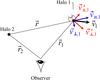Fig. 1 Geometry of halo pairs with respect to an observer. Velocities parallel or transverse to the line of sight (${\mathit{v}}_{\mathrm{\parallel }}^{\mathrm{\prime }}\mathit{,}{{v}}_{\mathrm{\perp }}^{\mathrm{\prime }}$) are shown in red, while velocities parallel or transverse to the connecting vector r between the halos (v∥,v⊥) are shown in blue.

Typically, only the line-of-sight (LOS) component of the velocity can be measured observationally, but v_∥ clearly depends on components both parallel and transverse to the LOS for a general pair geometry. As such, some form of deprojection method is needed to recover estimates of v_∥ and ${\mathit{\sigma }}_{\mathrm{\parallel }}^{\mathrm{2}}$ from data. Ferreira et al. (1999) achieved this by deriving an estimator for the mean radial velocity purely in terms of the observable LOS velocities and angles, 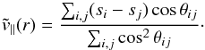$\begin{array}{c}\mathrm{˜}\\ {\mathit{v}}_{\mathrm{\parallel }}\end{array}\mathrm{\left(}\mathit{r}\mathrm{\right)}\mathrm{=}\frac{{\sum }_{\mathit{i,j}}\mathrm{(}{\mathit{s}}_{\mathit{i}}\mathrm{-}{\mathit{s}}_{\mathit{j}}\mathrm{)}\cos {\mathit{\theta }}_{\mathit{ij}}}{{\sum }_{\mathit{i,j}}{\cos }^{\mathrm{2}}{\mathit{\theta }}_{\mathit{ij}}}\mathrm{·}$(8)A distant-observer approximation has been used, such that $\cos {\mathit{\theta }}_{\mathit{ij}}\mathrm{\equiv }\hat{{r}}\mathrm{·}\hat{{l}}$, where $\hat{{l}}\mathrm{\equiv }\hat{{r}}{}_{\mathit{i}}\mathrm{\approx }\hat{{r}}{}_{\mathit{j}}$. Note that Ferreira et al. (1999) used a slightly different definition, $\hat{{l}}\mathrm{\equiv }\mathrm{(}\hat{{r}}{}_{\mathit{i}}\mathrm{+}\hat{{r}}{}_{\mathit{j}}\mathrm{)}\mathit{/}\mathrm{2}$, which is the mean of the LOS directions. Summations are performed over all pairs within a given separation bin, r_n ≤ r<r_{n + 1}.

We are unaware of an equivalent estimator for the dispersion, and so derive one in Appendix A, obtaining 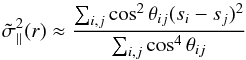$\stackrel{}{{{\mathit{\sigma }}_{\mathrm{\parallel }}^{\mathrm{2}}}_{\mathrm{˜}}}\mathrm{\left(}\mathit{r}\mathrm{\right)}\mathrm{\approx }\frac{{\sum }_{\mathit{i,j}}{\cos }^{\mathrm{2}}{\mathit{\theta }}_{\mathit{ij}}\mathrm{(}{\mathit{s}}_{\mathit{i}}\mathrm{-}{\mathit{s}}_{\mathit{j}}{\mathrm{)}}^{\mathrm{2}}}{{\sum }_{\mathit{i,j}}{\cos }^{\mathrm{4}}{\mathit{\theta }}_{\mathit{ij}}}$(9)in the limit of small θ_ij. More general expressions, including an estimator for the transverse dispersion, $\stackrel{}{{{\mathit{\sigma }}_{\mathrm{\perp }}^{\mathrm{2}}}_{\mathrm{˜}}}\mathrm{\left(}\mathit{r}\mathrm{\right)}$, are given in Appendix A.

We note that $\stackrel{}{{{\mathit{\sigma }}_{\mathrm{\parallel }}^{\mathrm{2}}}_{\mathrm{˜}}}\mathrm{\left(}\mathit{r}\mathrm{\right)}$ is different from the quantity ${\mathit{\sigma }}_{\mathrm{12}}^{\mathrm{2}}\mathrm{(}\mathrm{=}{\mathit{\sigma }}_{\mathrm{los}}^{\mathrm{2}}\mathrm{)}$ used by Hellwing (2014). The latter was defined by the Virgo Consortium (1998) as a quantity that is “somewhat closer to measurements accessible in galaxy redshift surveys” than the actual radial dispersion, ${\mathit{\sigma }}_{\mathrm{\parallel }}^{\mathrm{2}}\mathrm{\left(}\mathit{r}\mathrm{\right)}$. In our notation, ${\mathit{\sigma }}_{\mathrm{los}}^{\mathrm{2}}\mathrm{\left(}{\mathit{r}}_{\mathrm{p}}\mathrm{\right)}\mathrm{\equiv }\frac{\underset{\mathrm{-}\mathrm{\infty }}{\overset{\mathrm{\infty }}{\mathrm{\int }}}\mathit{\xi }\mathrm{\left(}\mathit{r}\mathrm{\right)}\hspace{0.17em}\mathrm{[}\frac{\mathrm{1}}{\mathrm{2}}{\sin }^{\mathrm{2}}{\mathit{\theta }}_{\mathit{ij}}\hspace{0.17em}{\mathit{\sigma }}_{\mathrm{\perp }}^{\mathrm{2}}\mathrm{+}{\cos }^{\mathrm{2}}{\mathit{\theta }}_{\mathit{ij}}\hspace{0.17em}\mathrm{(}{\mathit{\sigma }}_{\mathrm{\parallel }}^{\mathrm{2}}\mathrm{-}\mathrm{⟨}{\mathit{v}}_{\mathrm{\parallel }}{\mathrm{⟩}}^{\mathrm{2}}{\mathrm{\left)}}^{\mathrm{\right]}}\mathrm{d}\mathit{l}}{\underset{\mathrm{-}\mathrm{\infty }}{\overset{\mathrm{\infty }}{\mathrm{\int }}}\mathit{\xi }\mathrm{\left(}\mathit{r}\mathrm{\right)}\mathrm{d}\mathit{l}}\mathit{,}$(10)where ${\mathit{r}}_{\mathrm{p}}\mathrm{\equiv }\mathit{r}\sin {\mathit{\theta }}_{\mathit{ij}}\mathrm{=}\sqrt{{\mathit{r}}^{\mathrm{2}}\mathrm{-}{\mathit{l}}^{\mathrm{2}}}$ is the projected pair separation, ξ(r) is the halo correlation function, and the integration is along the LOS direction. The term in square brackets is the (centered) projected velocity dispersion, equivalent to the LOS velocity dispersion for a given pair geometry (r,l). In our notation, ${\mathit{\sigma }}_{\mathrm{\perp }}^{\mathrm{2}}$ is the centered variance of v_⊥. The factor of $\frac{\mathrm{1}}{\mathrm{2}}$ arises because one component of v_⊥ is orthogonal to the LOS and therefore does not contribute to the LOS dispersion. The integration over the LOS in Eq. (10) is equivalent to an ensemble average over all pairs with the same r_p, where ξ acts as a weight factor (normalized in the denominator) that specifies the fraction of pairs with separation r. In the ensemble, we therefore have ${\mathit{\sigma }}_{\mathrm{los}}^{\mathrm{2}}\mathrm{\left(}{\mathit{r}}_{\mathrm{p}}\mathrm{\right)}\mathrm{\equiv }\sum _{\mathit{i,j}}\mathrm{(}{\mathit{s}}_{\mathit{i}}\mathrm{-}{\mathit{s}}_{\mathit{j}}{\mathrm{)}}^{\mathrm{2}}\mathrm{-}{\left(\sum _{\mathit{i,j}}\mathrm{(}{\mathit{s}}_{\mathit{i}}\mathrm{-}{\mathit{s}}_{\mathit{j}}\mathrm{)}\right)}^{\mathrm{2}}\mathit{,}$(11)where the sums are over all pairs with fixed r_p. While this is an observable, as claimed by Virgo Consortium (1998), it is not a direct estimate of the variance of v_∥ as our estimator $\stackrel{}{{{\mathit{\sigma }}_{\mathrm{\parallel }}^{\mathrm{2}}}_{\mathrm{˜}}}$ is, and we therefore did not use it here.

In the remainder of the paper, we use the true radial velocity dispersion ${\mathit{\sigma }}_{\mathrm{\parallel }}^{\mathrm{2}}$, calculated from the full 3D velocity information in the simulated halo catalogs. This can then be connected to observations using the estimator $\stackrel{}{{{\mathit{\sigma }}_{\mathrm{\parallel }}^{\mathrm{2}}}_{\mathrm{˜}}}$ from Eq. (9). In Fig. 2 we show a comparison between the two quantities for the ΛCDM simulation; the agreement is good, although $\stackrel{}{{{\mathit{\sigma }}_{\mathrm{\parallel }}^{\mathrm{2}}}_{\mathrm{˜}}}$ is naturally noisier.

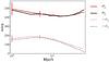Fig. 2 Comparison of the mean relative radial velocity, v∥(r), and the square root of its variance, σ∥(r), measured from ΛCDM simulation halos using full 3D information (red lines), and LOS-velocity estimators only (black lines). Quantities are shown in bins of pair separation, r. Bootstrap errors (68% CL) are shown for the r = (1,5) h-1 Mpc bins; we note that they are significantly larger than the differences between the black and red curves.

4. Measures of environment and screening

As discussed in Sect. 2, many modified gravity theories exhibit an environment-dependent screening of the fifth force. In this section, we describe a few possible ways of defining the environment of a dark matter halo, each of which is expected to trace the degree of screening in some way. These measures are then used to divide the simulated halo catalogs into multiple environment-dependent samples in Sect. 5.

4.1. Halo rescaling mass

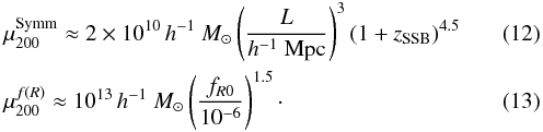
As shown in Gronke et al. (2015b), the halo mass itself is a fairly universal predictor of whether a halo is screened. Using an empirical fit of the fifth-force profiles of simulated halos with NFW density profiles, they defined the rescaling mass, μ₂₀₀, which is a characteristic mass scale above which the fifth force is expected to be screened. For a given theory, μ₂₀₀ is defined as the halo mass for which the mass-weighted mean of the fifth force in the halo is half its maximum (unscreened) strength. Partial screening is expected in a band of halo masses around μ₂₀₀. For the symmetron and f(R) models considered in this paper, Gronke et al. (2015b) found the fitting functions

$\begin{array}{ccc}& & \\ & & \end{array}$While these calculations are based on the strength of the fifth force affecting a test mass around an individual halo, the forces between nearby halos with similar masses can be expected to follow a similar pattern. This, in turn, will affect their clustering properties, so that we should expect clustering or velocity statistics for halos in mass bins well above the rescaling mass to be screened (i.e., reduced to their GR behavior). Conversely, halos in mass bins around or far below the rescaling mass will be partially or fully unscreened, respectively, so that deviations from GR should become apparent in the clustering statistics.

The values of the rescaling mass for each of the models considered here are given in Table 2. The f(R) models, even the weakest with f_R0 = 10^-6, have high rescaling masses, μ₂₀₀ ≥ 10¹³h^-1 M_⊙, which suggests that most halos from the simulations (which have typically much lower masses) should be partially or fully unscreened. The rescaling masses are substantially lower for all of the symmetron models except for super-early SSB, however, and a range of screening states are therefore expected for these models.

4.2. Isolatedness of halos

In the simple halo model, the properties of dark matter halos depend only on their mass. Evidence from observations and simulations suggests that the environment in which a halo forms is also important, however; an environment-dependent assembly bias (Croton et al. 2007) has been seen in the clustering of some observed galaxy samples, for example (Hearin et al. 2015). Various definitions of environment have been used to probe such effects, but many of them essentially reduce to proxies for halo mass (Haas et al. 2012). A more satisfactory definition of the environment of a halo is its isolatedness, which can be defined through (Haas et al. 2012) ${\mathit{D}}_{\mathit{N,f}}\mathrm{\equiv }\frac{{\mathit{d}}_{\mathit{N}}\mathrm{\left(}{\mathit{M}}_{\mathit{N}}\mathrm{\ge }\mathit{fM}\mathrm{\right)}}{{\mathit{r}}_{\mathit{N}}^{\mathrm{vir}}}\mathrm{·}$(14)Here, D_N,f is the distance from the halo to the Nth nearest neighbor whose mass exceeds f times the mass of the halo, divided by the virial radius of the neighbor, ${\mathit{r}}_{\mathit{N}}^{\mathrm{vir}}$. Halos with D_N,f greater than some threshold are considered to be isolated. This definition has the advantage of being insensitive to halo mass.

We follow Zhao et al. (2011) and Winther et al. (2012) in defining halos with D_1,1>10 to be isolated, which are those farther away from the nearest more-massive halo than ten times its virial radius. We also divide the halos into low-mass (5 × 10¹¹ ≤ M_halo ≤ 2 × 10¹²h^-1 M_⊙) and high-mass (M_halo> 2 × 10¹²h^-1 M_⊙) samples, resulting in a total of four bins in isolatedness (isolated vs. clustered) and mass (low vs. high).

It has been suggested in the literature (e.g., Zhao et al. 2011; Winther et al. 2012; Gronke et al. 2015a) that isolatedness is a proxy for the ambient density around the halo. This is not supported by our results, however (see Fig. 3 and Sect. 4.4, below), nor specifically by the original Haas et al. (2012) paper. Whether isolatedness is a useful measure of environment for studying modified gravity effects is also unclear: it has been found to correlate with chameleon-like screening by some authors (Zhao et al. 2011; Winther et al. 2012; Falck et al. 2015), but has also been found not to be associated with signs of screening by others (Gronke et al. 2015a).

4.3. Ambient density field

As discussed in Sect. 2, chameleon-like screening mechanisms respond to the ambient matter density: the fifth force vanishes in regions where ρ is sufficiently large. Binning halos according to their ambient density should therefore be a useful way of studying the screening behavior. The density distribution is scale-dependent, however, so that the mean density estimated over a finite region will depend on a smoothing scale related to the region size. The density that enters (e.g.) in the symmetron potential, Eq. (5), is a local quantity, with no implied averaging over extended regions, therefore it is not clear what smoothing scale to use for estimating ρ. This is not a problem in simulations because local values for the potential and field value are defined down to the simulation resolution.

For our problem, a reasonable choice is to consider the density field smoothed on scales on the order of the inter-halo separation, since this is the smallest scale on which we can reliably construct an estimate of the density field from a halo catalog. This can be consistently estimated by performing a Delaunay triangulation (Delaunay 1934) on the point distribution of halos, which is similar to a full Delaunay tessellation field estimation (Schaap & van de Weygaert 2000). Delaunay triangulation creates a set of tetrahedra that covers the volume spanned by the halo catalog, with each vertex coinciding with the position of a halo. The triangulation yields smaller tetrahedra around halos in regions with a high halo number density (i.e., many neighbors) and larger ones around more isolated halos. Dividing the halo mass by the volumes of the tetrahedra connected to that halo gives a point-wise measure of density (Martinez et al. 2009), 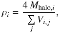${\mathit{\rho }}_{\mathit{i}}\mathrm{=}\frac{\mathrm{4}\hspace{0.17em}{\mathit{M}}_{\mathrm{halo}\mathit{,i}}}{\sum _{\mathit{j}}{\mathit{V}}_{\mathit{i,j}}}\mathit{,}$(15)where the index j labels the (connected) Delaunay tetrahedra, and the factor of 4 is a dimensional normalization constant, resulting from the fact that each tetrahedron is counted four times. The sum W_i = ∑ _jV_i,j is called the contiguous Voronoi cell around point i. This definition of point-wise density ensures that integrating the density over the simulation space yields the total mass of the halos used.

The ambient density contrast δ_i at point i is defined by (1 + δ_i) = , where is the mean density. We use six bins in δ in our analysis, as summarized in Table 3 and shown in Fig. 3. We performed Delaunay triangulation by using a MATLAB routine, which in turn uses the Computational Geometry Algorithms Library, CGAL (CGAL Project 2015).

4.4. Relationship between environment measures

Isolatedness (Eq. (14)) and ambient density (Eq. (15)) are expected to measure environment in substantially different ways. The former is constructed to be independent of halo mass, for example, while the latter will be correlated with mass, since high-mass halos tend to form in regions of higher density (Haas et al. 2012; Grützbauch et al. 2011; Chen et al. 2015).

Figure 3 shows the isolatedness measure D_1,1 against ambient density for all halos in the ΛCDM simulation above a minimum mass cutoff. The correlation between the two measures is weak (correlation coefficient r = 0.03), with each density bin containing halos of a wide range of isolatedness. Even the highest density bin (δ ≥ 10) contains a substantial fraction of isolated halos. Nevertheless, there is a slight tendency for isolated halos to form in regions of low density, which is presumably due to the difficulty of forming more than one massive halo in voids.

This means that we expect some measures of environment to be more effective markers of screened regions or halos than others. Since the chameleon-like screening in symmetron models has an explicit dependence on the local density, we would expect the binning in ambient density δ_i to exhibit the clearest differences in observables between screened and unscreened regions (although this will also be correlated with mass-dependent effects). We compare the effectiveness of the different measures in distinguishing screened and unscreened models in the following section.

5. Results

In this section, we investigate the dependence of the velocity statistics on halo mass, isolatedness, and ambient density for each of the simulated modified gravity models. We mostly focus on the quantity Δσ_∥ (see Sect. 3), which is the fractional deviation of the radial velocity dispersion from its GR+ΛCDM value (where we define Δ_X = X_MG/X_GR−1 for quantity X).

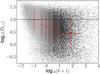Fig. 3 Isolatedness vs. ambient density for halos of mass Mhalo≥ 5 ×1011h-1 M⊙, taken from the ΛCDM simulation. The horizontal line divides the isolated (log 10D1,1 ≥ 1) and clustered subsamples. The gray shading of the points denotes the binning in ambient density; red errorbars denote the mean and standard deviation of the ambient density and isolatedness in each ambient density bin.

5.1. Dependence on halo mass

In Fig. 4 we show the absolute value and fractional deviation from GR for four different statistics, binned by halo mass with the binning specified in Table 3. Each bin is shown for two different halo pair separations, r = 1 and 5 h^-1 Mpc. We focus on r = 5 h^-1 Mpc below because the 1 h^-1 Mpc bin is considerably noisier (cf. the bootstrap errors in Fig. 2). Note that the noise due to sample variance is correlated between models because the simulations share the same initial conditions. Nevertheless, we include both in the figures to facilitate comparison with equivalent results in Hellwing et al. (2014).

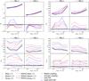Fig. 4 Comparison of statistics across models: ξ(r) (top left panel), v∥(r) (top right), σ∥(r) (bottom left), and σlos(r) (bottom right). The left and right columns in each panel are for pair separations r = 1 and 5h-1 Mpc, respectively. The upper rows show absolute values of the statistics, while the lower rows show the fractional deviation from GR (ΔX = XMG/XGR−1 for quantity X). The red points are taken from the f(R) model results presented in Hellwing et al. (2014). (These authors binned in M200c, the mass measured at the radius where Δ = 200 with respect to critical density; throughout this paper, we have consistently used M200b, which is measured with respect to the background matter density. The difference in the curves when M200c is used is negligible, however.)

The upper left panel of Fig. 4 shows the halo-halo correlation function, ξ_hh(r), estimated using the Landy-Szalay estimator (Landy & Szalay 1993), with 7000−30 000 halos per mass bin (Table 3). There is a clear trend of increasing correlation with mass for all models, which is expected; more massive halos are more strongly biased. The deviation Δξ becomes larger and more negative as we go from the weak to the strong f(R) model, indicating a suppression of clustering on these scales. A similar but more confused picture can be seen for the symmetron models. There is no clear evidence for a dependence of Δξ on mass, although there is a spike feature in the second mass bin for all models. This is most likely due to a large scatter in the neighboring mass bins, which we tentatively observed through a (50:50) subsampling of each bin. Clearer trends in ξ as a function of mass are observed by Hellwing et al. (2014) because they averaged over six different realizations of the initial fluctuations; they found no strong evidence for a mass dependence either.

The upper right panel of Fig. 4 shows the mean relative radial velocity, v_∥, in the same separation and mass bins. The Δv_∥ curves are more clearly separated for the different MG theories, with stronger modifications consistently giving larger fractional deviations. The dispersion of v_∥ is shown in the lower left panel. This quantity was calculated from the full 3D information in the simulations, not the estimator $\begin{array}{c}{\mathrm{˜}}_{}\\ {\mathit{\sigma }}_{\mathrm{\parallel }}\end{array}$. The pattern is more coherent than for the previous two quantities, with weaker modifications (e.g., weak f(R) and weaker coupling symmetron) exhibiting Δσ_∥ ≈ 0, and stronger modifications (e.g. strong f(R)) giving up to ~ 30% deviations from GR. Again, there is no clear dependence on mass, either of σ_∥ or Δσ_∥.

Finally, the lower right panel of Fig. 4 shows the dispersion of the relative LOS velocity, σ_los. As for σ_∥, the trend with increasing strength of deviation from GR is clear, and the dependence on mass is weak (although σ_los can be seen to decrease slightly with increasing mass). We also find that Δσ_∥ ≈ Δσ_los in all cases, with similar scatter across the mass bins. We find excellent agreement with the results for f(R) from Hellwing et al. (2014) (red points in Fig. 4) at a separation of r = 5 h^-1 Mpc, but less so at r = 1 h^-1 Mpc, where they observed a much stronger mass dependence.

Overall, then, we find no clear evidence that the fractional deviations of the velocity statistics depend on halo mass. This is qualitatively similar to what was found in Hellwing et al. (2014), although some of the results differ in detail. The lack of a strong mass dependence can be understood in terms of the fifth-force profiles calculated by Gronke et al. (2014) for the same symmetron and f(R) theories considered here. At distances beyond the virial radius, r ≥ r_vir, the fifth force was found to be approximately constant as a function of mass in all models when M_h ≲ 10¹³ M_⊙. (The fifth force decreases rapidly at higher M_h for some models, e.g., weak f(R), but is small in these models anyway, resulting in little overall change in velocity.)

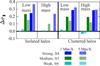Fig. 5 Fractional deviation from GR (Δσ∥ = σ∥ ,MG/σ∥ ,GR−1) of the relative radial velocity dispersion, Δσ∥, for the three f(R) models, binned by isolatedness (isolated vs. clustered) and mass (low and high halo mass) as described in Sect. 4.2. Pair separations r = 1 and 5 h-1 Mpc are presented with bold and pale shading, respectively. The isolated high-mass halo bin was excluded for r = 1h-1 Mpc because of the low number of halos within in.

5.2. Dependence on isolatedness

Figures 5 and 6 show the fractional deviations of the relative radial velocity dispersion, Δσ_∥, in bins of halo mass and isolatedness, D_1,1. As discussed in Sect. 4.2, halos are considered isolated when the nearest more-massive halo is greater than ten times its virial radius away, D_1,1> 10, and clustered otherwise. The boundary between the low- and high-mass bins is at 2 × 10¹²h^-1 M_⊙. As before, the results are presented for two halo separations, r = 1 and 5 h^-1 Mpc. We note that in some cases there are too few halo pairs at 1 h^-1 Mpc separation in the isolated bin, so these bins were removed from the plot.

Figure 5 shows Δσ_∥ for the f(R) models. For separations of r = 5 h^-1 Mpc, Δσ_∥ depends strongly on f_R0 for both clustered and isolated halos; the weak f(R) model (f_R0 = 10^-6) hardly deviates from GR, while strong f(R) (f_R0 = 10^-4) shows a ~ 30% deviation in both mass bins. At this separation, we see no clear dependence of Δσ_∥ on isolatedness, although there is tentative evidence for mass-dependence in the isolated bin (the strong f(R) model gives Δσ_∥ ≈ 35% and 23% in the low- and high-mass bins, respectively). This can potentially be explained by noise, however, as the isolated bins contain relatively fewer halo pairs. Noise also explains the relative scatter in the results for r = 1 h^-1 Mpc.

A clear dependence on isolatedness is found for one of the symmetron models, however (Fig. 6). For r = 5 h^-1 Mpc, the deviation for the stronger coupling symmetron model in the isolated bin is significant (~ 10−15%), but goes to zero in the clustered bin. A mild dependence on mass can also be seen in the isolated bin. The effect is much smaller for the weaker coupling model, which goes from a slightly positive (isolated) to slightly negative (clustered) deviation. These two models have the same z_SSB = 1 but differ in coupling strength by a factor of 2. For the other two symmetron models, there is no strong dependence on isolatedness; early SSB shows only a slight decrease in Δσ_∥ from the isolated to clustered bin, while a slight increase is observed for super-early SSB. The super-early SSB model shows a higher deviation overall.

Since SSB of the background occurred at a much earlier stage in these models (z_SSB = 2 and 3), we can expect the clustering of dark matter halos to have evolved with an active coupling between the scalar field and matter for a long time regardless of environment on cosmological scales, with screening only having been significant on very small scales. The environment dependence seen in the stronger coupling model may therefore have been erased (Gronke et al. 2014).

5.3. Dependence on ambient density

Figures 7 and 8 show the fractional deviation Δσ_∥ for each theory as a function of ambient density contrast, δ (see Sect. 4.3). Also plotted is the mean mass of halos in each bin, ⟨ M_h ⟩, divided by the rescaling mass μ₂₀₀ for each theory (see Sect. 2). Bins with 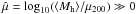are expected to contain halos that are screened, while highly negative values of are in the unscreened regime and therefore should correlate with stronger modified gravity effects (Gronke et al. 2015b). Between these two extremes, a band around corresponds to partial screening (orange shading in the figures). In this region, the screening mechanism is active, but deviations from GR are not fully suppressed; this is the transition region between the fully screened and unscreened states.

This relationship between screening and rescaled halo mass appears to be borne out by the figures. The Δσ_∥ curves for the strong and medium f(R) theories (Fig. 8) are flat, indicating no significant dependence on δ. Since is below the screening transition region for almost all of the ambient density bins, this is to be expected: both of these theories are fully unscreened across the whole range of δ, which means that no environment-dependent screening is taking place. This is not the case for the weak f(R) model, for which most of the bins are inside the transition region, screening should be partially active, but this also exhibits a flat Δσ_∥ curve. This model gives too small a modification in the first place for any environment dependence to be noticeable, however.

Fig. 6 Fractional deviation Δσ∥ for the four symmetron models (see Fig. 5 for key).

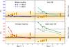Fig. 7 Fractional deviation from GR (Δσ∥ = σ∥ ,MG/σ∥ ,GR−1) for the four symmetron models (colored lines) for separations r = 1 (solid lines) and 5 h-1 Mpc (dashed) as a function of ambient density, δ. Deviations without binning in δ are shown as solid (r = 1 h-1 Mpc) and dashed (r = 5 h-1 Mpc) horizontal gray lines. Yellow points are the ratio of the mean halo mass to the rescaling mass (right axis; see Sect. 2), with the bars denoting the standard deviation within the bin, and the orange shading representing the band of partial screening found in Gronke et al. (2015b).

The symmetron models show a broader range of behavior (Fig. 7). In all cases and for all ambient density bins, is within the screening transition region (which is also wider than for the f(R) models). This suggests that environment-dependent screening should be observable for all four models, and this is indeed the case: the stronger coupling, early SSB, and super-early SSB models all show a strong evolution of Δσ_∥ with ambient density. The largest deviations occur in low-density (void) regions, with differences from GR+ΛCDM of up to 50% being observed for the super-early SSB model. The deviations are much smaller at high values of δ, as the symmetry of the scalar field potential is restored and the fifth force is suppressed. A ~ 20% deviation is observed even in the δ ≥ 10 bin for super-early SSB, however, as this model is generally closer to being unscreened than the others. The weaker coupling symmetron model does not fit into this pattern, showing Δσ_∥ ≈ 0 across the full δ range. As with the weak f(R) model, this may have more to do with the relative weakness of the modification to GR in this theory (although we note that it is not a weak modification in an absolute sense, as the matter power spectrum deviates from its GR behavior significantly on non-linear scales).

While the value of relative to the screening transition region appears to give a satisfactory explanation of our results, we cannot exclude the possibility that the behavior of the Δσ_∥ curves is unrelated to the mass of the individual halos. An alternative explanation is that (a) Δσ_∥ responds directly to the screening state in the region between the halos; and (b) the link between Δσ_∥ and halo mass is a secondary effect caused by the weak dependence of halo mass on ambient density. In this scenario, the internal structure or screening state of the halos themselves does not matter; the mass dependence is just a coincidence which is due to the expectation from the peak-background split formalism (Bardeen et al. 1986) that high-mass halos can form more readily in higher-density environments (see Table 3 for the mean halo mass and bias of each ambient density bin).

If this were the case, splitting each ambient density bin into high- and low-mass samples would yield similar Δσ_∥ curves. The dependence of σ_∥ on mass is more or less flat (Sect. 5.1), which means that if ambient density is the only factor, the results for the two mass bins should be the same. Conversely, if the value of with respect to the transition regime is important, then the different mass bins will give different results depending on how deep they are into the transition region.

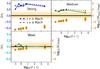Fig. 8 Fractional deviation Δσ∥ for the three f(R) models (colored lines; left axis), and the ratio of mean halo mass to rescaling mass (yellow points; right axis); see Fig. 7 for key.

Regardless of the reason, Figs. 7 and 8 show a clear environmental dependence of Δσ_∥ that differs between modified gravity theories. This is a tell-tale signature of screening at work. Moreover, all of the quantities involved are observables, making it possible to look for these signatures in forthcoming velocity surveys.

6. Discussion

We used N-body simulations of seven different modified gravity theories (three f(R) and four symmetron models) to investigate the dependence of a pairwise peculiar velocity statistic (the relative radial velocity dispersion, σ_∥) on halo environment. Strong environmental dependence is a key property of screening mechanisms – non-linear effects that are invoked by many MG theories to evade stringent local constraints on deviations from GR. By binning σ_∥ by a measure of environment (ambient density), we were able to observe signs of a transition from the screened to unscreened regimes for several of the theories we considered. The signatures differ markedly between models, with the f(R) theories presenting an essentially constant deviation of σ_∥ from its GR value, and the symmetron models showing a strong evolution of the deviation with density.

We chose to focus on the σ_∥ statistic because it is sensitive to modified-gravity effects on the typical scale of the screening transition, that is, around the inter-halo separation scale. A related statistic, the line-of-sight velocity dispersion σ_los, was also shown to be sensitive to modified gravity effects in Hellwing et al. (2014), although its environmental dependence was not considered. It is also less directly related to the relative radial velocity, v_∥, a physically meaningful quantity on which many velocity statistics are based. We compared these statistics in Sect. 3, where we also described an estimator for σ_∥ that makes this quantity observable.

In Sect. 4.4 we showed that two measures of halo environment, the isolatedness of halos, D_1,1, and the ambient density contrast, δ, are fundamentally different, contrary to some claims in the literature. To study screening effects at least, we obtained more coherent results when binning by ambient density (Sect. 5.3). This matches expectations for symmetron theories, where the local density is explicitly responsible for restoring the broken symmetry that activates the screening mechanism (Eq. (5)). Binning in isolatedness also revealed an environmental dependence on σ_∥, but the results were harder to interpret.

Throughout, we have worked under the assumption that noise-free distances and velocities are available for all dark matter halos down to some mass cutoff. Typical distance or velocity errors from peculiar velocity surveys are of the order of tens of percent, however (Tully et al. 2013), and scale poorly with redshift, which limits the survey volume. As such, current precision peculiar velocity samples are relatively limited in size, with the largest compilations containing only ~ afew × 10³ objects (Tully et al. 2013), which is most likely too small to see these effects. In addition, real-world measurements are obviously performed on galaxies and not dark matter halos, which complicates the process of associating subsamples with distinct mass bins. This also introduces a selection function that must be taken into account when (e.g.) correcting for Malmquist-type biases (Ferreira et al. 1999). Selection effects will presumably also be important in the reconstruction of the ambient density field (Sect. 4.3). Finally, the simulations we used did not take into account baryonic effects, which could also introduce environment-dependent signatures into the velocity field (although the recent work by Hellwing et al. 2016, suggests that baryonic effects have a relatively small effect on halo velocities at the scales considered here).

While an observational campaign to detect environment-dependent screening effects in the velocity field would clearly be more complex than the simple analysis we have presented here, there are no fundamental obstacles to its execution. All of the quantities we considered are closely related to observables (cf. Fig. 2) and can be accessed through the design of appropriate estimators (Appendix A). Furthermore, large homogeneously selected peculiar velocity surveys are planned for the near future, with optical and radio surveys expected to yield samples of 1−5 × 10⁴ objects over a substantial fraction of the sky (Koda et al. 2014). Alternative methods of measuring the velocity dispersion in an environment-dependent manner, for example, with redshift-space distortions, may also prove viable. We leave the question of the practical observability of these effects to future work.

In conclusion, we have presented a possible method for observing the screening transition in modified-gravity theories using the relative velocities of pairs of halos or galaxies and a density-based measure of halo environment. The signatures of deviations from GR are clear and depend on the particular modified gravity theory. The details of the signal and its ability to distinguish between different signals, will also depend on the properties of the peculiar velocity survey that is used, however; an investgation of this dependence is left to future work.

Acknowledgments

We are grateful to A. Barreira, B. Falck, M. Grönke, P. Lilje, H. Winther, H.-Y. Wu, and especially the referee, W. Hellwing, for useful comments and discussions, and R. O. Fauli for preliminary work during a masters project. PB’s research was supported by an appointment to the NASA Postdoctoral Program at the Jet Propulsion Laboratory, California Institute of Technology, administered by Universities Space Research Association under contract with NASA. DFM is supported by the Research Council of Norway. We thank NOTUR for proving computational support.

References

Appendix A: Pairwise velocity estimators

For a given halo pair geometry, the variance of the relative velocity of the pair, v_i−v_j, projected along the LOS, is ${\mathit{\sigma }}_{\mathrm{los}}^{\mathrm{2}}\mathrm{=}\frac{\mathrm{1}}{\mathrm{2}}{\sin }^{\mathrm{2}}\mathit{\theta }\hspace{0.17em}\stackrel{}{{{\mathit{\sigma }}_{\mathrm{\perp }}^{\mathrm{2}}}_{\mathrm{˜}}}\mathrm{\left(}\mathit{r,l}\mathrm{\right)}\mathrm{+}{\cos }^{\mathrm{2}}\mathit{\theta }\hspace{0.17em}\mathrm{\left[}\stackrel{}{{{\mathit{\sigma }}_{\mathrm{\parallel }}^{\mathrm{2}}}_{\mathrm{˜}}}\mathrm{\right(}\mathit{r,l}\mathrm{)}\mathrm{-}\mathrm{(}\begin{array}{c}\mathrm{˜}\\ {\mathit{v}}_{\mathrm{\parallel }}\end{array}\mathrm{\left(}\mathit{r,l}\mathrm{\right)}{\mathrm{)}}^{\mathrm{2}}\mathrm{]}\mathit{,}$(A.1)where we have used ⟨ v_⊥ ⟩ = 0. An empirical estimate of this quantity can be obtained by summing over many halo pairs with the same geometry, ${\mathit{\sigma }}_{\mathrm{los}\mathit{,}\mathrm{obs}}^{\mathrm{2}}\mathrm{=}\sum _{\mathit{i,j}}\mathrm{(}{\mathit{s}}_{\mathit{i}}\mathrm{-}{\mathit{s}}_{\mathit{j}}{\mathrm{)}}^{\mathrm{2}}\mathrm{-}{\left(\sum _{\mathit{i,j}}\mathrm{(}{\mathit{s}}_{\mathit{i}}\mathrm{-}{\mathit{s}}_{\mathit{j}}\mathrm{)}\right)}^{\mathrm{2}}\mathit{.}$(A.2)Following a similar strategy to Ferreira et al. (1999), we construct a simple estimator for ${\mathit{\sigma }}_{\mathrm{\parallel }}^{\mathrm{2}}$ by writing ${\mathit{\chi }}^{\mathrm{2}}\mathrm{=}\sum \mathrm{(}{\mathit{\sigma }}_{\mathrm{los}\mathit{,}\mathrm{obs}}^{\mathrm{2}}\mathrm{-}{\mathit{\sigma }}_{\mathrm{los}}^{\mathrm{2}}{\mathrm{)}}^{\mathrm{2}}$, where the sums are now over all pairs with fixed separation, r. We then minimize with respect to ${\mathit{\sigma }}_{\mathrm{\parallel }}^{\mathrm{2}}$ by setting $\mathrm{d}{\mathit{\chi }}^{\mathrm{2}}\mathit{/}\mathrm{d}\mathrm{\left(}{\mathit{\sigma }}_{\mathrm{\parallel }}^{\mathrm{2}}\mathrm{\right)}\mathrm{=}\mathrm{0}$, and rearrange to obtain $\stackrel{}{{{\mathit{\sigma }}_{\mathrm{\parallel }}^{\mathrm{2}}}_{\mathrm{˜}}}\mathrm{=}\frac{{\sum }_{\mathit{i,j}}{\cos }^{\mathrm{2}}{\mathit{\theta }}_{\mathit{ij}}\mathrm{\left[}\mathrm{\right(}{\mathit{s}}_{\mathit{i}}\mathrm{-}{\mathit{s}}_{\mathit{j}}{\mathrm{)}}^{\mathrm{2}}\mathrm{-}\frac{\mathrm{1}}{\mathrm{2}}\stackrel{}{{{\mathit{\sigma }}_{\mathrm{\perp }}^{\mathrm{2}}}_{\mathrm{˜}}}{\sin }^{\mathrm{2}}{\mathit{\theta }}_{\mathit{ij}}\mathrm{-}\stackrel{}{{{\mathit{v}}_{\mathrm{\parallel }}^{\mathrm{2}}}_{\mathrm{˜}}}\mathrm{(}\mathrm{1}\mathrm{-}{\cos }^{\mathrm{2}}{\mathit{\theta }}_{\mathit{ij}}{\mathrm{\left)}}^{\mathrm{\right]}}}{{\sum }_{\mathit{i,j}}{\cos }^{\mathrm{4}}{\mathit{\theta }}_{\mathit{ij}}}\mathrm{·}$(A.3)An estimate of $\begin{array}{c}{\mathrm{˜}}_{}\\ {\mathit{v}}_{\mathrm{\parallel }}\end{array}$ can be obtained using Eq. (8), and $\stackrel{}{{{\mathit{\sigma }}_{\mathrm{\perp }}^{\mathrm{2}}}_{\mathrm{˜}}}$ by performing the minimization $\mathrm{d}{\mathit{\chi }}^{\mathrm{2}}\mathit{/}\mathrm{d}\mathrm{\left(}{\mathit{\sigma }}_{\mathrm{\perp }}^{\mathrm{2}}\mathrm{\right)}\mathrm{=}\mathrm{0}$. After rearranging and combining with Eq. (A.3), we obtain

$\begin{array}{ccc}& & \stackrel{}{{{\mathit{\sigma }}_{\mathrm{\parallel }}^{\mathrm{2}}}_{\mathrm{˜}}}\mathrm{\left(}\mathit{r}\mathrm{\right)}\mathrm{=}[\left(\sum _{\mathit{i,j}}{\sin }^{\mathrm{4}}{\mathit{\theta }}_{\mathit{ij}}\right)\left(\sum _{\mathit{i,j}}{\cos }^{\mathrm{2}}{\mathit{\theta }}_{\mathit{ij}}\mathrm{(}{\mathit{s}}_{\mathit{i}}\mathrm{-}{\mathit{s}}_{\mathit{j}}{\mathrm{)}}^{\mathrm{2}}\right)\\ & & \mathrm{-}\hspace{0.17em}\left(\sum _{\mathit{i,j}}{\cos }^{\mathrm{2}}{\mathit{\theta }}_{\mathit{ij}}{\sin }^{\mathrm{2}}{\mathit{\theta }}_{\mathit{ij}}\right)\left(\sum _{\mathit{i,j}}{\sin }^{\mathrm{2}}{\mathit{\theta }}_{\mathit{ij}}\mathrm{(}{\mathit{s}}_{\mathit{i}}\mathrm{-}{\mathit{s}}_{\mathit{j}}{\mathrm{)}}^{\mathrm{2}}\right)]\\ & & \mathrm{\times }\hspace{0.17em}{\left[\left(\sum _{\mathit{i,j}}{\cos }^{\mathrm{4}}{\mathit{\theta }}_{\mathit{ij}}\right)\left(\sum _{\mathit{i,j}}{\sin }^{\mathrm{4}}{\mathit{\theta }}_{\mathit{ij}}\right)\mathrm{-}{\left(\sum _{\mathit{i,j}}{\cos }^{\mathrm{2}}{\mathit{\theta }}_{\mathit{ij}}{\sin }^{\mathrm{2}}{\mathit{\theta }}_{\mathit{ij}}\right)}^{\mathrm{2}}\right]}^{-1}\end{array}$(A.4)

and $\begin{array}{ccc}& & \stackrel{}{{{\mathit{\sigma }}_{\mathrm{\perp }}^{\mathrm{2}}}_{\mathrm{˜}}}\mathrm{\left(}\mathit{r}\mathrm{\right)}\mathrm{=}\mathrm{2}\hspace{0.17em}[\left(\sum _{\mathit{i,j}}{\cos }^{\mathrm{4}}{\mathit{\theta }}_{\mathit{ij}}\right)\left(\sum _{\mathit{i,j}}{\sin }^{\mathrm{2}}{\mathit{\theta }}_{\mathit{ij}}\mathrm{(}{\mathit{s}}_{\mathit{i}}\mathrm{-}{\mathit{s}}_{\mathit{j}}{\mathrm{)}}^{\mathrm{2}}\right)\\ & & \mathrm{-}\hspace{0.17em}\left(\sum _{\mathit{i,j}}{\cos }^{\mathrm{2}}{\mathit{\theta }}_{\mathit{ij}}{\sin }^{\mathrm{2}}{\mathit{\theta }}_{\mathit{ij}}\right)\left(\sum _{\mathit{i,j}}{\cos }^{\mathrm{2}}{\mathit{\theta }}_{\mathit{ij}}\mathrm{(}{\mathit{s}}_{\mathit{i}}\mathrm{-}{\mathit{s}}_{\mathit{j}}{\mathrm{)}}^{\mathrm{2}}\right)]\\ & & \mathrm{\times }\hspace{0.17em}{\left[\left(\sum _{\mathit{i,j}}{\cos }^{\mathrm{4}}{\mathit{\theta }}_{\mathit{ij}}\right)\left(\sum _{\mathit{i,j}}{\sin }^{\mathrm{4}}{\mathit{\theta }}_{\mathit{ij}}\right)\mathrm{-}{\left(\sum _{\mathit{i,j}}{\cos }^{\mathrm{2}}{\mathit{\theta }}_{\mathit{ij}}{\sin }^{\mathrm{2}}{\mathit{\theta }}_{\mathit{ij}}\right)}^{\mathrm{2}}\right]}^{-1}\mathrm{-}\mathrm{2}\hspace{0.17em}\stackrel{}{{{\mathit{v}}_{\mathrm{\parallel }}^{\mathrm{2}}}_{\mathrm{˜}}}\mathrm{\left(}\mathit{r}\mathrm{\right)}\mathit{.}\end{array}$(A.5)Note that these expressions do not account for the noise in the LOS velocity measurements, which will increase the variance (and therefore must be taken into account in any real measurement).

All Tables

All Figures

	Fig. 1 Geometry of halo pairs with respect to an observer. Velocities parallel or transverse to the line of sight (${\mathit{v}}_{\mathrm{\parallel }}^{\mathrm{\prime }}\mathit{,}{{v}}_{\mathrm{\perp }}^{\mathrm{\prime }}$) are shown in red, while velocities parallel or transverse to the connecting vector r between the halos (v∥,v⊥) are shown in blue.
In the text

Fig. 2 Comparison of the mean relative radial velocity, v∥(r), and the square root of its variance, σ∥(r), measured from ΛCDM simulation halos using full 3D information (red lines), and LOS-velocity estimators only (black lines). Quantities are shown in bins of pair separation, r. Bootstrap errors (68% CL) are shown for the r = (1,5) h-1 Mpc bins; we note that they are significantly larger than the differences between the black and red curves.

In the text

	Fig. 3 Isolatedness vs. ambient density for halos of mass Mhalo≥ 5 ×1011h-1 M⊙, taken from the ΛCDM simulation. The horizontal line divides the isolated (log 10D1,1 ≥ 1) and clustered subsamples. The gray shading of the points denotes the binning in ambient density; red errorbars denote the mean and standard deviation of the ambient density and isolatedness in each ambient density bin.
In the text

Fig. 4 Comparison of statistics across models: ξ(r) (top left panel), v∥(r) (top right), σ∥(r) (bottom left), and σlos(r) (bottom right). The left and right columns in each panel are for pair separations r = 1 and 5h-1 Mpc, respectively. The upper rows show absolute values of the statistics, while the lower rows show the fractional deviation from GR (ΔX = XMG/XGR−1 for quantity X). The red points are taken from the f(R) model results presented in Hellwing et al. (2014). (These authors binned in M200c, the mass measured at the radius where Δ = 200 with respect to critical density; throughout this paper, we have consistently used M200b, which is measured with respect to the background matter density. The difference in the curves when M200c is used is negligible, however.)

In the text

Fig. 5 Fractional deviation from GR (Δσ∥ = σ∥ ,MG/σ∥ ,GR−1) of the relative radial velocity dispersion, Δσ∥, for the three f(R) models, binned by isolatedness (isolated vs. clustered) and mass (low and high halo mass) as described in Sect. 4.2. Pair separations r = 1 and 5 h-1 Mpc are presented with bold and pale shading, respectively. The isolated high-mass halo bin was excluded for r = 1h-1 Mpc because of the low number of halos within in.

In the text

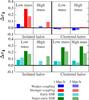	Fig. 6 Fractional deviation Δσ∥ for the four symmetron models (see Fig. 5 for key).
In the text

Fig. 7 Fractional deviation from GR (Δσ∥ = σ∥ ,MG/σ∥ ,GR−1) for the four symmetron models (colored lines) for separations r = 1 (solid lines) and 5 h-1 Mpc (dashed) as a function of ambient density, δ. Deviations without binning in δ are shown as solid (r = 1 h-1 Mpc) and dashed (r = 5 h-1 Mpc) horizontal gray lines. Yellow points are the ratio of the mean halo mass to the rescaling mass (right axis; see Sect. 2), with the bars denoting the standard deviation within the bin, and the orange shading representing the band of partial screening found in Gronke et al. (2015b).

In the text

	Fig. 8 Fractional deviation Δσ∥ for the three f(R) models (colored lines; left axis), and the ratio of mean halo mass to rescaling mass (yellow points; right axis); see Fig. 7 for key.
In the text

References

- Amendola, L., & Tsujikawa, S. 2010, Dark energy: theory and observations (Cambridge University Press) [Google Scholar]
- Baker, T., Psaltis, D., & Skordis, C. 2015, ApJ, 802, 63 [NASA ADS] [CrossRef] [Google Scholar]
- Bardeen, J. M., Bond, J. R., Kaiser, N., & Szalay, A. S. 1986, ApJ, 304, 15 [NASA ADS] [CrossRef] [Google Scholar]
- Barreira, A., Li, B., Hellwing, W. A., Baugh, C. M., & Pascoli, S. 2013, J. Cosmol. Astropart. Phys., 10, 027 [Google Scholar]
- Behroozi, P. S., Wechsler, R. H., & Wu, H.-Y. 2013, ApJ, 762, 109 [NASA ADS] [CrossRef] [Google Scholar]
- Brax, P. 2013, Class. Quant. Grav., 30, 214005 [NASA ADS] [CrossRef] [Google Scholar]
- Brax, P., & Davis, A.-C. 2015, J. Cosmol. Astropart. Phys., 10, 042 [Google Scholar]
- Brax, P., Davis, A.-C., Li, B., & Winther, H. A. 2012, Phys. Rev. D, 86, 044015 [NASA ADS] [CrossRef] [Google Scholar]
- Bull, P., Akrami, Y., Adamek, J., et al. 2016, Physics of the Dark Universe 12, 56 [Google Scholar]
- CGAL Project 2015, CGAL User and Reference Manual (CGAL Editorial Board) [Google Scholar]
- Chen, Y.-C., Ho, S., Mandelbaum, R., et al. 2015, ArXiv e-prints [arXiv:1509.06376] [Google Scholar]
- Clampitt, J., Cai, Y.-C., & Li, B. 2013, MNRAS, 431, 749 [NASA ADS] [CrossRef] [Google Scholar]
- Clifton, T., Ferreira, P. G., Padilla, A., & Skordis, C. 2012, Phys. Rep., 513, 1 [NASA ADS] [CrossRef] [MathSciNet] [Google Scholar]
- Clifton, T., Mota, D. F., & Barrow, J. D. 2005, MNRAS, 358, 601 [NASA ADS] [CrossRef] [Google Scholar]
- Croton, D. J., Gao, L., & White, S. D. M. 2007, MNRAS, 374, 1303 [NASA ADS] [CrossRef] [Google Scholar]
- Davis, M., & Peebles, P. J. E. 1977, ApJS, 34, 425 [NASA ADS] [CrossRef] [Google Scholar]
- Davis, A.-C., Li, B., Mota, D. F., & Winther, H. A. 2012, ApJ, 748, 61 [NASA ADS] [CrossRef] [Google Scholar]
- Delaunay, B. 1934, Bulletin de l’Académie des Sciences de l’URSS, 793 [Google Scholar]
- Falck, B., Koyama, K., & Zhao, G.-B. 2015, J. Cosmol. Astropart. Phys., 7, 049 [NASA ADS] [CrossRef] [Google Scholar]
- Ferreira, P. G., Juszkiewicz, R., Feldman, H. A., Davis, M., & Jaffe, A. H. 1999, ApJ, 515, L1 [NASA ADS] [CrossRef] [Google Scholar]
- Gorski, K. 1988, ApJ, 332, L7 [NASA ADS] [CrossRef] [Google Scholar]
- Gronke, M., Llinares, C., Mota, D. F., & Winther, H. A. 2015a, MNRAS, 449, 2837 [NASA ADS] [CrossRef] [Google Scholar]
- Gronke, M., Mota, D. F., & Winther, H. A. 2015b, A&A, 583, A123 [NASA ADS] [CrossRef] [EDP Sciences] [Google Scholar]
- Gronke, M. B., Llinares, C., & Mota, D. F. 2014, A&A, 562, A9 [NASA ADS] [CrossRef] [EDP Sciences] [Google Scholar]
- Grützbauch, R., Conselice, C. J., Varela, J., et al. 2011, MNRAS, 411, 929 [NASA ADS] [CrossRef] [Google Scholar]
- Haas, M. R., Schaye, J., & Jeeson-Daniel, A. 2012, MNRAS, 419, 2133 [NASA ADS] [CrossRef] [Google Scholar]
- Hand, N., Addison, G. E., Aubourg, E., et al. 2012, Phys. Rev. Lett., 109, 041101 [NASA ADS] [CrossRef] [Google Scholar]
- Hearin, A. P., Watson, D. F., & van den Bosch, F. C. 2015, MNRAS, 452, 1958 [NASA ADS] [CrossRef] [Google Scholar]
- Hellwing, W. A. 2014, ArXiv e-prints [arXiv:1412.8738] [Google Scholar]
- Hellwing, W. A., Cautun, M., Knebe, A., Juszkiewicz, R., & Knollmann, S. 2013, J. Cosmol. Astropart. Phys., 10, 012 [Google Scholar]
- Hellwing, W. A., Barreira, A., Frenk, C. S., Li, B., & Cole, S. 2014, Phys. Rev. Lett., 112, 22 [Google Scholar]
- Hellwing, W. A., Schaller, M., Frenk, C. S., et al. 2016, MNRAS, 461, L11 [NASA ADS] [CrossRef] [Google Scholar]
- Hinterbichler, K., & Khoury, J. 2010, Phys. Rev. Lett., 104, 23 [Google Scholar]
- Hinterbichler, K., Khoury, J., Levy, A., & Matas, A. 2011, Phys. Rev. D, 84, 10 [Google Scholar]
- Hu, W., & Sawicki, I. 2007, Phys. Rev. D, 76, 6 [Google Scholar]
- Jain, B., Vikram, V., & Sakstein, J. 2013, ApJ, 779, 39 [NASA ADS] [CrossRef] [Google Scholar]
- Joyce, A., Jain, B., Khoury, J., & Trodden, M. 2015, Phys. Rep., 568, 1 [NASA ADS] [CrossRef] [MathSciNet] [Google Scholar]
- Juszkiewicz, R., Springel, V., & Durrer, R. 1999, ApJ, 518, L25 [NASA ADS] [CrossRef] [Google Scholar]
- Juszkiewicz, R., Ferreira, P. G., Feldman, H. A., Jaffe, A. H., & Davis, M. 2000, Science, 287, 109 [NASA ADS] [CrossRef] [Google Scholar]
- Koda, J., Blake, C., Davis, T., et al. 2014, MNRAS, 445, 4267 [NASA ADS] [CrossRef] [Google Scholar]
- Landy, S. D., & Szalay, A. S. 1993, ApJ, 412, 64 [NASA ADS] [CrossRef] [Google Scholar]
- Li, B., Hellwing, W. A., Koyama, K., et al. 2013, MNRAS, 428, 743 [NASA ADS] [CrossRef] [Google Scholar]
- LIGO Collaboration, & Virgo Collaboration 2016, Phys. Rev. Lett., 116, 221101 [NASA ADS] [CrossRef] [PubMed] [Google Scholar]
- Llinares, C., Zhao, H. S., & Knebe, A. 2009, ApJ, 695, L145 [NASA ADS] [CrossRef] [Google Scholar]
- Llinares, C., Mota, D. F., & Winther, H. A. 2014, A&A, 562, A78 [NASA ADS] [CrossRef] [EDP Sciences] [Google Scholar]
- Lombriser, L., Schmidt, F., Baldauf, T., et al. 2012, Phys. Rev. D, 85, 102001 [NASA ADS] [CrossRef] [Google Scholar]
- Lombriser, L., Simpson, F., & Mead, A. 2015, Phys. Rev. Lett., 114, 251101 [NASA ADS] [CrossRef] [PubMed] [Google Scholar]
- Ma, Y.-Z., Li, M., & He, P. 2015, A&A, 583, A52 [NASA ADS] [CrossRef] [EDP Sciences] [Google Scholar]
- Martinez, J. V., Saar, E., Gonzales, M. E., & Pons-Borderia, J. M. 2009, Data Analysis in Cosmology, eds. J. V. Martinez, E. Saar, M. E. Gonzales, & J. M. Pons-Borderia (Berlin, Heidelberg: Springer), 291 [Google Scholar]
- Martino, M. C., & Sheth, R. K. 2009, ArXiv e-prints [arXiv:0911.1829] [Google Scholar]
- Oyaizu, H., Lima, M., & Hu, W. 2008, Phys. Rev. D, 78, 123524 [NASA ADS] [CrossRef] [Google Scholar]
- Pietroni, M. 2005, Phys. Rev. D, 72, 043535 [NASA ADS] [CrossRef] [Google Scholar]
- Planck Collaboration XIV. 2016, A&A, 594, A14 [NASA ADS] [CrossRef] [EDP Sciences] [Google Scholar]
- Schaap, W. E., & van de Weygaert, R. 2000, A&A, 363, L29 [NASA ADS] [Google Scholar]
- Schmidt, F., Lima, M., Oyaizu, H., & Hu, W. 2009, Phys. Rev. D, 79, 083518 [NASA ADS] [CrossRef] [Google Scholar]
- Scoccimarro, R. 2004, Phys. Rev. D, 70, 083007 [NASA ADS] [CrossRef] [Google Scholar]
- Sheth, R. K., & Diaferio, A. 2001, MNRAS, 322, 901 [Google Scholar]
- Shirata, A., Shiromizu, T., Yoshida, N., & Suto, Y. 2005, Phys. Rev. D, 71, 064030 [NASA ADS] [CrossRef] [Google Scholar]
- Stark, A., Miller, C. J., Kern, N., et al. 2016, Phys. Rev. D, 93, 084036 [NASA ADS] [CrossRef] [Google Scholar]
- Teyssier, R. 2010, Astrophysics Source Code Library [record ascl:1011.007] [Google Scholar]
- Tully, R. B., Courtois, H. M., Dolphin, A. E., et al. 2013, AJ, 146, 86 [NASA ADS] [CrossRef] [Google Scholar]
- Virgo Consortium 1998, ApJ, 499, 20 [NASA ADS] [CrossRef] [Google Scholar]
- Will, C. M. 2014, Liv. Rev. Relativ., 17 [Google Scholar]
- Winther, H. A., Mota, D. F., & Li, B. 2012, ApJ, 756, 166 [NASA ADS] [CrossRef] [Google Scholar]
- Wyman, M., Jennings, E., & Lima, M. 2013, Phys. Rev. D, 88, 084029 [NASA ADS] [CrossRef] [Google Scholar]
- Zhao, G.-B. 2014, ApJS, 211, 23 [NASA ADS] [CrossRef] [Google Scholar]
- Zhao, G.-B., Li, B., & Koyama, K. 2011, Phys. Rev. Lett., 107, 071303 [NASA ADS] [CrossRef] [Google Scholar]