| Issue |
A&A
Volume 595, November 2016
|
|
|---|---|---|
| Article Number | A90 | |
| Number of page(s) | 14 | |
| Section | Numerical methods and codes | |
| DOI | https://doi.org/10.1051/0004-6361/201628578 | |
| Published online | 03 November 2016 | |
Discontinuous Galerkin finite element methods for radiative transfer in spherical symmetry
1 Physikalisches Institut &
Center for Space and Habitability, University of Bern, Sidlerstr. 5, 3012 Bern, Switzerland
e-mail: This email address is being protected from spambots. You need JavaScript enabled to view it.
2 Zentrum für Astronomie und
Astrophysik, Technische Universität Berlin, Hardenbergstr. 36, 10623
Berlin,
Germany
Received:
23
March
2016
Accepted:
24
July
2016
Abstract
The discontinuous Galerkin finite element method (DG-FEM) is successfully applied to treat a broad variety of transport problems numerically. In this work, we use the full capacity of the DG-FEM to solve the radiative transfer equation in spherical symmetry. We present a discontinuous Galerkin method to directly solve the spherically symmetric radiative transfer equation as a two-dimensional problem. The transport equation in spherical atmospheres is more complicated than in the plane-parallel case owing to the appearance of an additional derivative with respect to the polar angle. The DG-FEM formalism allows for the exact integration of arbitrarily complex scattering phase functions, independent of the angular mesh resolution. We show that the discontinuous Galerkin method is able to describe accurately the radiative transfer in extended atmospheres and to capture discontinuities or complex scattering behaviour which might be present in the solution of certain radiative transfer tasks and can, therefore, cause severe numerical problems for other radiative transfer solution methods.
Key words: radiative transfer / methods: numerical / stars: atmospheres
© ESO 2016
1. Introduction
Many stars, such as asymptotic giant branch (AGB) stars, have extended atmospheres, which has important physical and observational implications. In particular, the radiation field at large distances from the inner stellar disk becomes very dilute and is confined primarily to a narrow solid angle around the radial direction (Mihalas 1978). Additionally, planets can also feature extended atmospheres, in which case the use of the usual assumption of a plane-parallel atmosphere is no longer valid, for example, the extended and spherically stratified atmosphere of Pluto (Gladstone et al. 2016). Compared to the radiative transfer equation in the plane-parallel approximation, the transfer equation in spherical symmetry is more complicated and more difficult to handle. This is especially caused by the appearance of a derivative with respect to the polar angle, which is not present in the plane-parallel geometry. Other cases in which the plane-parallel radiative transfer equation becomes much more complicated include systems with a moving medium where photons are subject to the Doppler effect and aberration (Mihalas 1978).
Depending on the transport coefficients, the general radiative transport equation can have a very different mathematical character. As described in Kanschat et al. (2009), it is a hyperbolic wave equation in regions without matter, an elliptic diffusion equation in case of an optically thick medium, or a parabolic equation when the light is strongly peaked in the forward direction. It is, therefore, very difficult to find numerical methods which are capable of dealing with these different (or even mixed) types of behaviour.
The problem of a grey spherical atmosphere in radiative equilibrium was first studied by Kosirev (1934) and Chandrasekhar (1934). An extension of the iterative moment method for plane-parallel atmospheres using variable Eddington factors (Auer & Mihalas 1970) to the problem of a spherically symmetric atmosphere restricted to isotropic scattering was introduced by Hummer & Rybicki (1971). Additionally, solutions based on a generalised Eddington approximation were developed by Lucy (1971) and Unno & Kondo (1976), respectively.
Alternatively, the long (Cannon 1970) or short characteristic methods (Kunasz & Auer 1988) can be used. Combined with, for example, an operator perturbation method to account for the unknown source function – such as the accelerated lamdba iteration (Cannon 1973) – they can be used to solve the radiative transfer equation in multiple dimensions (Olson & Kunasz 1987; Kunasz & Olson 1988). In combination with the work of Hummer & Rybicki (1971), operator splitting methods have also been directly utilised for spherically symmetric atmospheres by Kubat (1994).
Currently, the computationally demanding Monte Carlo techniques can very efficiently solve the radiative transfer problem for a broad variety of applications ranging from stellar atmospheres (e.g. Abbott & Lucy 1985; Lucy & Abbott 1993; Lucy 1999), circumstellar disks (e.g. Pascucci et al. 2004, and the references therein), and supernovae (e.g. Lucy 2005) to dusty objects (e.g. Steinacker et al. 2013, and the references therein). Their advantages are, for example, that they are intrinsically three-dimensional, can handle easily complex geometries and density distributions, and have a low algorithmic complexity. However, in some special cases with very optically thick regions the Monte Carlo approach becomes very slow because the number of photon interactions (i.e. scattering) increases exponentially. In these situations grid-based solution techniques (e.g. a finite difference, finite element, or finite volume method) for the differential equation of radiative transfer are more favourable even if they are algorithmically quite complex. Moreover, grid-based techniques allow for higher order approximations as well as error control, and they can be formulated to be intrinsically flux conserving (Hesthaven & Warburton 2008; Henning 2001).
In this study, we present a numerical method for a direct solution of the radiative transfer equation in spherical symmetry by means of a finite element method. Finite element methods have already been used to solve the radiative transfer equation, most notably in the three-dimensional case by Kanschat (1996) or Richling et al. (2001). In these cases, a continuous Galerkin finite element was used to discretise the transport operator. Such an approach, however, causes problems in cases where the transport equation has a dominant hyperbolic character, which may lead to discontinuities within the solution. It is possible to stabilise the numerical scheme by introducing a streamline diffusion method, for example, which essentially transforms the hyperbolic equation into a parabolic one by adding a small diffusion in the direction of photon transport. While this stabilises the numerical discretisation, it also adds a free parameter to the method, which has to be chosen carefully in such a way that it stabilises the numerical scheme, but does not result in a decreased accuracy of the solution (see e.g. Eriksson et al. 1996; Kanschat 1996). An alternative way to deal with such problems is to soften the requirements for the solution of the finite element method, in particular the requirement of continuity of the solution across element boundaries. One such numerical approach in the context of finite element methods is the discontinuous Galerkin method.
The discontinuous Galerkin finite element method (DG-FEM) was first introduced by Reed & Hill (1973) to study neutron transport problems. Since then, the method has been successfully applied to a broad variety of parabolic, hyperbolic, and elliptic problems (e.g. Hesthaven & Warburton 2008; Cockburn 2003). For three-dimensional internal heat transfer problems, the discretisation with a discontinuous Galerkin method has been studied by Cui & Li (2004). For astrophysical applications, discontinuous Galerkin methods have, for example, been used by Dykema et al. (1996) and Castor et al. (1992).
In this work we use a DG-FEM to directly solve the radiative transfer equation with arbitrarily complex scattering phase functions in spherical symmetry as a two-dimensional problem. In contrast to other solution methods, the scattering integral can thereby be evaluated exactly, independent of the angular mesh resolution. The development of the numerical scheme is outlined for the formulation of the DG approach in Sects. 2 and 3. Its applicability to several test problems is presented in Sect. 4. Remarks on the numerical efficiency are given in Sect. 5, followed by an outlook (Sect. 6) and a summary (Sect. 7).
2. Radiative transfer equation
We consider the radiative transfer equation in spherical symmetry, cf. Mihalas (1978), i.e. 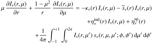 (1)with the specific intensity Iν, radius coordinate r, the cosine of the polar angle μ, the azimuth angle φ, absorption coefficient κν, total (
 ) and differential (sν(r,μ,μ′;φ,φ′)) scattering coefficients, and induced and spontaneous emission coefficients
  .
.
The differential scattering coefficient can be decomposed in an averaged angle-independent part, the total scattering coefficient  , and the phase function p(r,μ,μ′;φ,φ′). This yields
 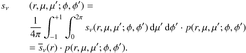 (2)The phase function describes the probability of photon scattering of incident directions μ′ and φ′ into the directions μ and φ. Since in spherical symmetry the radiation field is independent of the azimuth angle φ, the phase function p(r,μ,μ′;φ,φ′) can formally be integrated with respect to the azimuth angle to obtain the azimuthally averaged phase function
 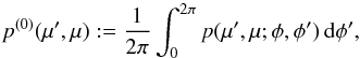 (3)which is then used in the transfer equation. To guarantee the conservation of energy, the phase function is normalised to unity, i.e.
 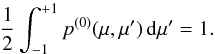 (4)The extinction coefficient
  can be combined with the induced emission into
  (5)In this work we only consider cases with
  and therefore
  , i.e. we do not consider systems which are dominated by induced emission (such as maser). Equation (1)is therefore simplified to
 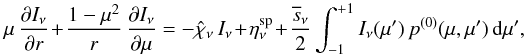 (6)where all direct dependences on r and μ have been omitted to simplify the presentation. Instead of the usual form of the radiative transfer equation in spherical symmetry given by Eq. (6), we use the mathematically equivalent form
 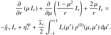 (7)To simplify the notation we drop the explicit frequency dependence in the transfer equation and its corresponding coefficients in the following. We do not introduce the usual (radial) optical depth in the transfer equation. Doing so – by moving the extinction coefficient
  to the left-hand side – would introduce additional terms of the form
  , which can be numerically destabilising since the extinction coefficient can vary over several orders of magnitude.
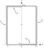 |
Fig. 1 Computational domain Ω. The boundaries of the domain between the inner radius rin and outer radius rout, as well as μ between + 1 and −1, are denoted by the respective Γ. |
The Eq. (7)is solved on the two-dimensional domain Ω ⊂ R2 with Ω ∋ x = (r,μ) ∈ (rin,rout) × (−1,1) as displayed in Fig. 1. The inner (outer) radius of Ω is given by rin (rout).
At the inner boundary Γin of the domain boundary conditions need to be imposed for positive values of μ, i.e. 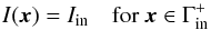 (8)given by the radiation field, for example, of the stellar interior. Likewise, at the outer boundary Γout an incident external radiation field has to be prescribed for negative values of μ, i.e.
 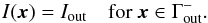 (9)We note that since the differential with respect to μ in Eq. (7)vanishes on the boundary ∂Γ, no explicit boundary conditions need to be imposed on Γμ±. Therefore, the boundary value problem considered in this work is given by
 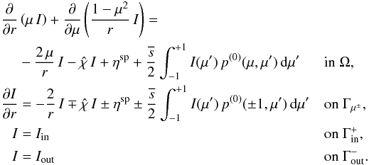 (10)
(10)
3. Formulation of the discontinuous Galerkin method
For the formulation of the discontinuous Galerkin method we follow the notation of Hesthaven & Warburton (2008). The domain Ω is described by K non-overlapping elements Dk, i.e.  (11)such that the continuous domain Ω is approximated by the finite domain Ωh with
 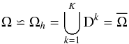 (12)with a local element size
hk:
= diam(Dk).
(12)with a local element size
hk:
= diam(Dk).
Definition 1. For any open set Ω in Rn let Pq(Ω) and Qq(Ω) denote the set of algebraic polynomials of total and partial degree ≤q, respectively. For n = 2 Table 1 shows the monomial basis functions of Pq and Qq for q = 0,1,2,3 and Fig. 2 displays their Lagrangian elements.
Monomial basis of polynomial spaces Pq and Qq of total and partial degree ≤ q, respectively, for n = 2, and q = 0,1,2,3.
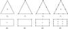 |
Fig. 2 Lagrangian reference elements for dimension n = 2, and polynomial degrees q = 0,1,2,3. The degrees of freedom (see Table 1) are marked with •. Top: Pq elements, bottom: Qq elements. |
In this work we use the nodal representation of the solution  on each element. For each element Dk a suitable set of local grid points
  is chosen and the local continuous solution of
  is expressed using the interpolating Lagrange polynomials, such that
 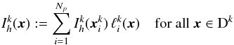 (13)is a polynomial of order q on each element. Here the so called trial functions
  are the interpolating two-dimensional Lagrange polynomials through the grid points
  , i.e.
 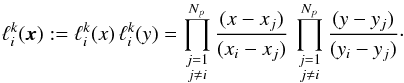 (14)For a given order q the number of local grid points Np is given by
 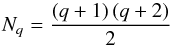 (15)for Pq elements and by
  (16)for Qq elements, respectively. In principle the polynomial order q and thus Np can vary from element to element. However, for simplicity of notation we assume here that all elements have the same order q. Subsequently, the set
  of the local grid point indices within each element k is denoted by
  (17)The global piecewise continuous solution can then be written as the direct sum of all K solutions
  (18)The trial functions
  introduced in Eq. (13)form a basis of the finite vector space Vh. This vector space is locally defined by
 and globally given by
  . Unlike the case of the continuous Galerkin finite element method (Eriksson et al. 1996), we note that no continuity of the trial functions (and therefore also of the solution I) is assumed or required across inter–element boundaries.
We define the residual of Eq. (10)by 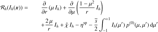 (19)with Ih ∈ Vh. In the context of finite element methods this residual is minimised with respect to all test functions
  in each element. This gives the weak formulation of Eq. (10), which represents the physical principle of virtual work. Thus, it is required that
  (20)For this study we consider only test functions, which are members of the same finite vector space as the trial functions, i.e.
  . This corresponds to a Ritz-Galerkin method (Hesthaven & Warburton 2008). We note that in principle
  may also be defined as a member of vector spaces other than
  (e.g. δ-distributions). The choice of different trial and test vector spaces leads to Petrov-Galerkin finite element schemes (Hesthaven & Warburton 2008) which are, however, not considered here.
For this particular choice of test functions we require for each element Dk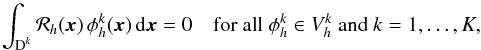 (21)i.e. the residual is required to be orthogonal to all test functions
  . Since the test functions are given by a linear combination of the Lagrange polynomials, i.e.
 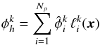 (22)with the expansion coefficients
  , Eq. (21)results in the Np equations
 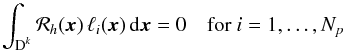 (23)on each element Dk.
In summary, we consider in this work the following DG(q)-method: Seek Ih ∈ Vh such that 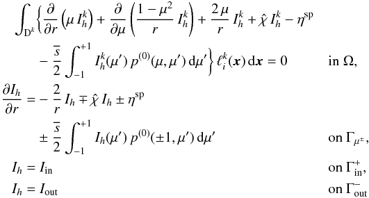 (24)for i = 1,...,Np and k = 1,...,K.
3.1. Elementwise calculations
Let us first consider the two terms  under the integral in Eq. (24). Using the expansion of the solution within one element k (see Eq. (13)) yields
 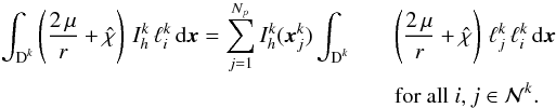 (25)This defines the local symmetric mass matrix
  with
with 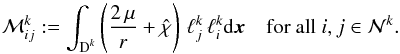 (26)The term ηsp in Eq. (24)simply yields the local load vector
  , with
 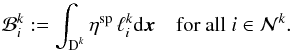 (27)Next we consider the differential with respect to r in Eq. (24). An integration by parts shifts the differential from the unknown quantity to the test function
  introducing an additional integral over the boundary of the element Dk, i.e.
 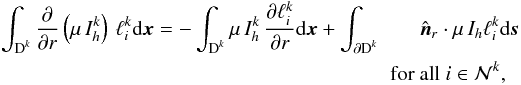 (28)where
  denotes the outward facing normal vector in r direction (see Fig. 3).
Because it is allowed to be discontinuous across element boundaries, the solution Ih is not uniquely defined at the boundary. Therefore, a numerical flux (f)∗ is introduced which describes the flow of information from one element to another, yielding 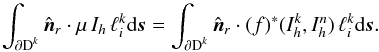 (29)The numerical flux depends in general on the solutions of the local element and the adjacent element
  and is directly related to the dynamics of the considered differential equation. For a particular choice of the flux a matrix ℱkn can be defined which contains the contributions due to the jump at the inter-element boundaries between the elements k and n. The exact contribution depends on the details of the numerical flux used, as discussed in Sect. 3.2.
Using again the expansion of Eq. (13)for the solution in the element k, the local stiffness matrix  can be introduced as
 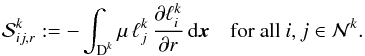 (30)For the differential with respect to μ in Eq. (24)integration by parts yields
 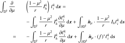 (31)for all
  and the respective outward facing normal vector in μ direction (see Fig. 3).
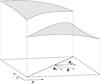 |
Fig. 3 Jump in the numerical solution along the normal |


The corresponding stiffness matrix is given by 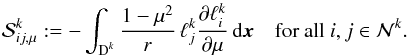 (32)The total local stiffness matrix
  for the element k can then be obtained by the sum of
  and
and  , i.e.
 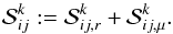 (33)
(33)
3.2. Numerical flux
The numerical flux considered here is the known as the upwind flux (e.g. Cockburn 2003; Hesthaven & Warburton 2008), given by 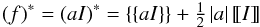 (34)with
  (35)as the average of the solutions and
  (36)as the jump of the solution along the normal. The situation is shown in Fig. 3, where the jump between two P2 elements is illustrated. The parameter a is here either given by
  (37)for the differential with respect to r, or by
  (38)for the differential with respect to μ. This particular flux was chosen because for the radiative transfer problem considered here information propagates only in the direction of photon travel. The upwind flux for radiative transfer problems has already been considered by e.g. Li (2006). We note, however, that the choice of this flux is not unique. Other fluxes with different properties may be used (see Cockburn 2003, for a review on DG fluxes). The connection between the test and trial functions of the adjacent elements can be written as a matrix
 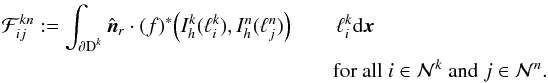 (39)Unlike the other matrices (such as ℳk), which are only defined over a single element, the matrix ℱkn connects a local element k with adjacent elements n. If the scattering integral considered below is not taken into account, this would be the only connection between different elements.
3.3. Scattering matrix
The contribution due to scattering in Eq. (24)is given by the integral 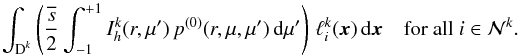 (40)Using the expansions from Eqs. (13)and (18)results in
 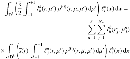 (41)for all and
  . This defines a matrix
  containing the contributions due to scattering
 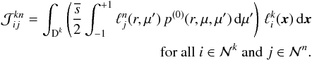 (42)We note that the scattering integral in Eq. (42)only contains known quantities, namely the scattering phase function p(0) and the Lagrange polynomials ℓj. Thus, the integral can be evaluated exactly for any arbitrary complex phase function, independent of the mesh resolution. This is a direct advantage over other radiative transfer methods, for example the discrete ordinate methods (Thomas & Stamnes 2002) where the evaluation of the scattering integral is directly coupled to the resolution of the angular mesh (Chandrasekhar 1960).
3.4. Transformation matrix
To assemble a global matrix for the solution of the resulting system of equations, the matrixes and tensors with the local indices i and j must be mapped onto a matrix with global indices. This is done via a transformation matrix  . Let g be a linear bijective mapping, which maps the set of local indices i within each element k onto a set
  of global coordinates
  (43)with
  (44)The linear mapping can be written as a transformation matrix
  . The matrix
  then maps, for example, the scattering matrix onto the global scattering matrix
  with the global indices α and β, which yields
 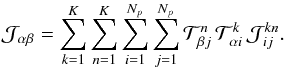 (45)The global mass matrix ℳ, stiffness matrix
  , and jump matrix ℱ can be obtained via the same process. The total left-hand side matrix
  of the linear system of equations can be expressed by
 (46)The resulting linear system of equations is then
  (47)with
  and ℬ the global load vector (cf. Eq. (27)). Since is a sparse matrix, the system can be efficiently solved by an iterative method (such as GMRES) and an appropriate pre-conditioner in many cases (Hackbusch 1994).
However, as mentioned by Kanschat & Meinköhn (2004) the matrix is sometimes badly conditioned, especially in cases with high opacity and single scattering albedos. The usual pre-conditioners (such as ILU, Hackbusch 1994) in combination with GMRES then fail to yield a converged solution. In this case a more adapted pre-conditioner is required to solve the system of Eq. (47). An example of such a pre-conditioner based on the Eddington approximation but limited to a plane-parallel situation is given by Kanschat & Meinköhn (2004). Nonetheless such a pre-conditioner should also be adaptable to spherically symmetric atmospheres which will be the subject of a forthcoming publication.
4. Test problems
In this section, we test our previously described numerical solution of the radiative transfer equation with a discontinuous Galerkin method. Due to the lack of exact solutions, we need to rely on test problems for comparison, where the resulting radiation field is known a priori, or to make a comparison with results of previously published calculations.
The first two tests evaluate the numerical stability and flux conservation in an empty atmosphere. In this case, the photons follow the characteristic paths of the transfer Eq. (1). These scenarios also feature discontinuities in their solutions, which will serve as a test for the numerical stability of our DG formulation.
For the third scenario, we refer to the radiative transfer calculations for an isotropically scattering, spherical atmosphere with a power-law extinction coefficient (Hummer & Rybicki 1971). We compare our results with their published values and also verify that the energy is also conserved in this case as required. We note that the intention of these calculations is to validate and verify the numerical approach and its capabilities to cope with discontinuities or highly scattering atmospheres, for example.
4.1. Computational details
We implemented the numerical algorithms described in the previous section by using the general finite element library GetFEM++1. In principle, the element-wise calculations can also be performed in the sense of Alberty et al. (1999). Details of our numerical implementation are given in the Appendix.
A DG(1) method on a structured grid with rectangular Q1 elements is used for the first two test problems. For both cases, the grid contains a total of 100 grid points in the radial direction and 80 grid points in the angular direction. The radius grid points are distributed equidistantly, while the angular mesh is constructed by using a Gaussian quadrature rule. The relatively high resolution is required to capture the discontinuous solutions properly. In principle, a much lower resolution could be used in these cases if an unstructured grid is constructed where the elements are directly aligned to capture the (previously) known discontinuities in the solution.
For the third test problem, we use a DG(2) method on a structured Q2 grid with 25 radial points and 10 angular values. The radial nodes are placed in logarithmic equidistant steps, while for the angular grid a Gaussian quadrature rule is again employed.
The resulting linear system of equations is solved by an iterative GMRES solver with a restart value of 10 in each case. The iteration matrix is preconditioned by an incomplete LU factorisation.
4.2. Empty atmospheres with an isotropically emitting inner surface
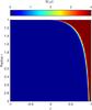 |
Fig. 4 Radiation field I(μ,r) as a function of radius r and angular variable μ for an empty, extended atmosphere with an isotropically emitting inner surface. |
As a very first test we study the following simple radiative transfer problem 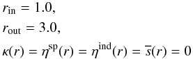 (48)with boundary conditions
  (49)which represents an empty, extended atmosphere with an isotropically emitting inner surface.
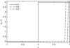 |
Fig. 5 Radiation field I(μ,r) as a function of the angular variable μ and three chosen radii r. The vertical dotted line denotes μc, the limiting value of μ under which the inner emitting surface is seen at the outer boundary r = 3. The discontinuity is accurately captured (i.e. the solution shows no oscillations). |
The resulting radiation field I(μ,r) is shown in Fig. 4. Additionally, several cuts through the parameter space are given in Fig. 5, where the intensity I is shown as a function of μ for three different values of r. We note that in this radiative transfer problem a real discontinuity is present in the solution which separates the region of constant intensity originating from the inner surface and the regions where the intensity is zero. The characteristic separating these two regions is given by  (50)The results in Figs. 4 and 5 clearly show the spherical dilution of the outward directed intensity. With increasing radius r the angle μc, under which the central emitting surface can be seen, decreases strongly. This is illustrated in greater detail in Fig. 5, where the intensity I is shown as a function of μ and for three different values of r. The vertical dotted line marks the limiting value of μc(rout) under which the emitting inner surface is seen at the outer boundary. As suggested by Fig. 5, the DG method presented here accurately reproduces this spherical dilution of the radiation field without introducing numerical oscillations.
Consequently, the DG method is capable of capturing this discontinuity quite well without introducing numerical oscillations which would occur in case of a continuous Galerkin method. In practice, the discontinuity is smeared out over one element. In order to limit the errors introduced by this out-smearing it is possible to use either high mesh resolution in general or adaptive mesh refinement along the discontinuous boundaries of the intensity given by Eq. (50).
Because there are no interactions of the atmosphere with the radiation field in this test example, the radiative transfer problem should be automatically energy conserving. For a spherically symmetric atmosphere this means that the flux (r2H(r)) is constant throughout the atmosphere, where H is the first angular moment (Eddington flux) of the intensity  (51)In this first test calculation, the flux is conserved better than 0.01% everywhere in the computational domain, indicating that the DG method is stable and accurate for such a problem.
4.3. Empty atmospheres illuminated by an exterior light source
This test case differs from the previous one only by choosing different boundary conditions  (52)This problem then represents an empty, extended atmosphere illuminated by an exterior light source. The particular form of the outer boundary condition has been chosen to highlight the photons’ characteristics, i.e. the geometric pathways of photons travelling through the atmosphere. The resulting radiation field is shown in Figs. 6 and 7.
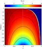 |
Fig. 6 Radiation field I(μ,r) as a function of radius r and angular variable μ for an empty, extended atmosphere illuminated by an exterior light source. The curved black lines illustrate a number of selected characteristics of this radiative transfer problem, i.e. the pathways of photons through the atmosphere. The vertical white line separates ingoing and outgoing directions. |
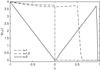 |
Fig. 7 Radiation field I(μ,r) as a function of the angular variable μ and three chosen radii r. The discontinuity is accurately captured (i.e. there are no oscillations in the solution). |
As can be clearly be seen in Fig. 6, only a small fraction of the incident radiation eventually reaches the inner surface. The remaining radiation is transmitted through the atmosphere and leaves the computational domain at the outer boundary with the same intensity and under the same angle as the incident radiation field. The curved black lines in Fig. 6 illustrate some of the characteristics of this radiative transfer problem, i.e. the pathways of photons through the atmosphere. This behaviour is very different to problems with plane-parallel geometry where the incident light under any angle would eventually reach the surface.
Like the previous test case, this radiative transfer problem also has a discontinuous solution in a part of its computational domain. This discontinuity is also captured accurately by the DG formulation introduced in this work (see Fig. 7). Again, the flux is conserved better than 0.01% everywhere in the computational domain.
4.4. Isotropically scattering atmosphere
To prove that our DG radiative transfer method can handle non-local scattering problems, we compare our results with calculations published in Hummer & Rybicki (1971) resembling a purely scattering, spherical atmosphere with a power-law opacity in this section. In contrast to our work, Hummer & Rybicki (1971) used an iterative moment method to obtain the solution of the radiative transfer equation, although owing to the limitation of this method, only isotropic scattering was taken into account. The radiative transfer problem considered here for comparison is therefore specified by 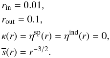 (53)Following Hummer & Rybicki (1971), scattering is assumed to be isotropic, i.e. the scattering phase function is given by
 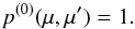 (54)Boundary conditions are chosen to resemble those introduced in Hummer & Rybicki (1971). The moment method employed by Hummer & Rybicki (1971) allowed for a direct prescription of the radiation flux at the inner boundary, which was set to
  . At the outer boundary, no incident radiation was assumed. To replicate these constant flux boundary conditions, we employed the following conditions on the specific intensity at the domain boundaries
  (55)This inner boundary condition is obtained from the requirement that
 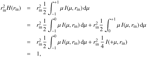 (56)assuming an isotropic distribution of I( + μ,rin).
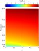 |
Fig. 8 Radiation field I(μ,r) as a function of radius r and angular variable μ. The vertical black line separates ingoing and outgoing directions. |
Because of the purely scattering atmosphere, the radiation flux r2H(r) needs to be conserved throughout the atmosphere. The resulting values of r2H(r) differ from the assumed constant flux at the inner boundary  by less than 0.5% everywhere in the computational domain. In the inner part of the atmosphere, the highest deviations are below 0.001% indicating again the capability of the DG method.
The resulting radiation field I(μ,r) is shown in Fig. 8. In contrast to the previous two test problems, no discontinuity occurs in this case. Owing to the many multiple scattering events, the radiation field exhibits a smooth behaviour in angle and radius. At the inner boundary, the radiation field is isotropic, resulting in an Eddington factor of 0.3 as expected.
Mean intensity.
Figure 9 shows the resulting values of the mean intensity r2J(r) in comparison to the corresponding tabulated values taken from Table II in Hummer & Rybicki (1971). Agreement with the results of Hummer & Rybicki (1971) are excellent in all parts of the isotropically scattering atmosphere. It should be noted that the grid resolution used in the present calculation is much lower than that employed by Hummer & Rybicki (1971) (200 r-points, 100 angles). We use a factor of eight fewer radius grid points and a factor of ten fewer angular values. The radiation field as a function of radius and angle is rather smooth and so does not require a high resolution – especially since the intensity here is assumed to be a second-order polynomial within each element.
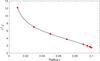 |
Fig. 9 Mean intensity r2J as a function of the radius for an isotropically scattering atmosphere. The dots mark the corresponding results published by Hummer & Rybicki (1971). |
Limb-darkening.
The limb-darkening curves  are shown in Fig. 10 as a function of the impact parameter
  , given by
  (57)The curve shows an excellent agreement with the results of Hummer & Rybicki (1971; their Fig. 6). The calculated disk centre intensity I(0) is 816.4, which deviates by less than 0.5% from the value of 820 given in Hummer & Rybicki (1971). We note, however, that their solution was stated to have a flux conservation error of a few percent at the outer boundary, while our flux is conserved better than 0.5% everywhere, which can explain the slight deviations in the disk centre intensity.
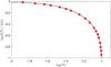 |
Fig. 10 Limb-darkening curve I(p) /I(0) as a function of the impact parameter |
5. Numerical efficiency
In this section we study the development of the computational time as a function of the total number of degrees of freedom N by using the previous, third test example for the DG(2) method (isotropic scattering atmosphere). We test separately the dependence on the number of angular and on radius points. Successively increasing the resolution in either grid direction, we track the development of the computational effort. For a grid composed of Qq elements with Nq local degrees of freedom N is given by 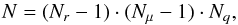 (58)where Nr and Nμ are the number of radial and angular grid points. According to
 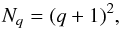 (59)the number of local degrees of freedom for the Q2 elements used here is nine (see Fig. 2). We note that the computational time includes every single step to solve the problem, from the construction of the grid and finding the corresponding elements throughout the grid that need to be connected by the scattering integral to calculating the element-wise contributions to the matrix and solving the linear system of equations. In reality, many of these tasks need to be done only once – such as the element connections – and their results can be re-used at different iteration steps or for other frequencies.
The corresponding results are shown in Fig. 11, which also depicts the corresponding linear fits through the obtained data points to determine the order of dependence on the grid point number. The results in Fig. 11 suggest that the computing time increases linearly with the number of radius points. For a smaller number of angles, the computational time increases with N1.5. For numbers of N larger than about 10 000, this dependency changes to N2.5 (see Fig. 11). For comparison, the iterative method using variable Eddington factors as employed by Hummer & Rybicki (1971) typically scales cubic in the number of radius grid points for one iteration step Mihalas (1978), if for each radius point a corresponding tangent ray (equal to two angular directions) is used. Several iterations, however, are needed to obtain a converged solution, which means that the overall computational cost is larger than this estimate.
It should be noted that with increasing numbers of degrees of freedom, most of the time is spent solving the linear system of equations. This is, in fact, the main reason for the increase in the computational time for the angular points. The scattering integral (Eq. (42)) is responsible for connecting elements in the final matrix which are, however, not direct neighbours in the grid. Depending on the actual implementation of the element numbering scheme (and, thus their position in ), the contributions to the integral Eq. (42)by those elements can be scattered throughout the matrix . This makes an efficient solution of the linear system of equations quite hard for an iterative solver. A considerable decrease in computing time could, therefore, be obtained when the element numbering scheme would take the elements’ connections due to the scattering integral into account, such that the contributions of these elements would be located closer to the main diagonal of the matrix (see e.g. Cuthill & McKee 1969). For a purely scattering atmosphere, we were able to obtain converged solutions up to optical depths of around 100. Beyond that, the matrix becomes too badly conditioned to be solved by a standard GMRES scheme with an ILU preconditioner. As mentioned in Sect. 3.4, a more sophisticated preconditioner needs to be developed for such cases.
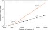 |
Fig. 11 Development of the normalised computational time as a function of the number of degrees of freedom. Both variables are depicted in logarithmic scale. The black dots mark the results for increasing the number of radius grid points from 40 to 500, while the number of angles is kept constant at 10. The red crosses indicate the results for increasing the angular resolution from 10 to 82, using a constant radial grid point number of 40. The corresponding solid lines depict the linear fits through the respective data points. For the angular nodes, two different fits are used. |
6. Outlook
The implementation of the DG-FEM presented in this work can be greatly extended in the future in view of its numerical efficiency. One improvement which can be addressed is adaptive grid refinement in combination with error estimation. To this end, the residual in Eq. (23)provides the opportunity of obtaining an a posteriori error estimate. The pointwise error of the calculated solution can be estimated by expressing this equation in a suitable norm. In regions where the error is above a certain threshold, a local grid refinement or a local increase of the polynomial order can then be used to increase the numerical accuracy. Using this adaptive grid refinement ensures that the exact solution is calculated accurately on the entire grid. Adaptive mesh refinement can become important when the solution features a non-monotonous intensity distribution. This can occur within circumstellar dust shells, for example, where the dust forming region somewhere in the atmosphere creates a local maximum in the angular intensity distribution (Gail & Sedlmayr 2014). Such a non-monotonous behaviour can easily be traced by local grid refinement without increasing the resolution in other parts of the grid.
Another option for improving the numerical efficiency of the presented DG-FEM is to parallelise the numerical work. In principle, since the DG-FEM formulation does not enforce continuity across element boundaries, all element-wise calculations presented in Sect. 3.1 can be computed independently from each other. Thus, such independent computations can be parallelised very easily by using MPI or OpenMP schemes, for example. Furthermore, the calculations within each element – unless pushed to very high orders – are always a comparatively small numerical problem. Such small problems are ideal for running on GPU clusters, i.e. graphic card processors with thousands of cores, which could increase the computational speed by at least one order of magnitude.
Finally, the solution of the final linear system of equations can also be parallised. Special libraries, such as PETSc, are available to distribute the computational task across several CPUs or GPUs. This would be especially helpful in cases where most of the time is spent by the iterative solver.
7. Summary
In this work we presented a numerical method to directly solve the radiative transfer equation in spherical symmetry. We used a discontinuous Galerkin finite element method to discretise the transport equation as a two-dimensional boundary value problem. Arbitrary complex scattering phase function can, in particular, be integrated exactly using this approach. The discretisation yields a sparse system of equations which can be solved by standard iterative methods with suitable preconditioners.
The applicability of the DG-FEM is verified on a set of different test problems. The discontinuous Galerkin method is able to directly describe the spherical dilution of the radiation field in an extended atmosphere. We show that the DG-FEM is able to accurately capture discontinuities which might appear in the solution of the transfer equation for special test problems. We also compared our method with previously published radiative transfer calculations for a spherical, isotropically scattering atmosphere. The agreement between the different approaches was found to be excellent. Consequently, the discontinuous Galerkin method is perfectly suitable for treating accurately the radiative transfer in a spherical atmosphere even with, for example, discontinuities in the radiation field or complex scattering behaviour, which might cause severe numerical problems for other radiative transfer solution methods.
Acknowledgments
D.K. gratefully acknowledges the support of the Center for Space and Habitability of the University of Bern and the MERAC Foundation for partial financial assistance. This work has been carried out within the frame of the National Centre for Competence in Research PlanetS supported by the Swiss National Science Foundation. D.K. acknowledges the financial support of the SNSF. The authors thank the anonymous referee for the very constructive and helpful comments that greatly improved the manuscript.
References
- Abbott, D. C., & Lucy, L. B. 1985, ApJ, 288, 679 [NASA ADS] [CrossRef] [Google Scholar]
- Alberty, J., Carstensen, C., & Funken, S. 1999, Numerical Algorithms, 20, 117 [NASA ADS] [CrossRef] [MathSciNet] [Google Scholar]
- Auer, L. H., & Mihalas, D. 1970, MNRAS, 149, 65 [NASA ADS] [Google Scholar]
- Cannon, C. J. 1970, ApJ, 161, 255 [NASA ADS] [CrossRef] [Google Scholar]
- Cannon, C. J. 1973, J. Quant. Spec. Radiat. Transf., 13, 627 [NASA ADS] [CrossRef] [Google Scholar]
- Castor, J. I., Dykema, P. G., & Klein, R. I. 1992, ApJ, 387, 561 [NASA ADS] [CrossRef] [Google Scholar]
- Chandrasekhar, S. 1934, MNRAS, 94, 444 [NASA ADS] [CrossRef] [Google Scholar]
- Chandrasekhar, S. 1960, Radiative transfer (New York: Dover) [Google Scholar]
- Cockburn, B. 2003, Z. Angew. Math. Mech., 83, 731 [CrossRef] [MathSciNet] [Google Scholar]
- Cui, X., & Li, B. 2004, Num. Heat Transfer Part B – Fundamentals, 46, 399 [NASA ADS] [CrossRef] [Google Scholar]
- Cuthill, E., & McKee, J. 1969, in Proc. 24th National Conference, ACM ’69 (New York, NY, USA: ACM), 157 [Google Scholar]
- Dykema, P. G., Klein, R. I., & Castor, J. I. 1996, ApJ, 457, 892 [NASA ADS] [CrossRef] [Google Scholar]
- Eriksson, K., Estep, D., Hansbo, P., & Johnson, C. 1996, Computational Differential Equations (Cambridge University Press) [Google Scholar]
- Gail, H.-P., & Sedlmayr, E. 2014, Physics and Chemistry of Circumstellar Dust Shells (Cambridge University Press) [Google Scholar]
- Gladstone, G. R., Stern, S. A., Ennico, K., et al. 2016, Science, 351, 8866 [Google Scholar]
- Hackbusch, W. 1994, Iterative solution of large sparse systems of equations, Applied mathematical sciences (Berlin: Springer) [Google Scholar]
- Henning, T. 2001, in The Formation of Binary Stars, eds. H. Zinnecker, & R. Mathieu, IAU Symp., 200, 567 [Google Scholar]
- Hesthaven, J. S., & Warburton, T. 2008, Nodal Discontinuous Galerkin Methods: Algorithms, Analysis, and Applications, Texts in Applied Mathematics (Springer) [Google Scholar]
- Hummer, D. G., & Rybicki, G. B. 1971, MNRAS, 152, 1 [NASA ADS] [CrossRef] [Google Scholar]
- Kanschat, G. 1996, Ph.D. Thesis, University of Heidelberg and preprint 96−29, IWR Heidelberg [Google Scholar]
- Kanschat, G., & Meinköhn, E. 2004, SFB359 Preprints (University of Heidelberg) [Google Scholar]
- Kanschat, G., Meinköhn, E., Rannacher, R., & Wehrse, R. 2009, Numerical Methods in Multidimensional Radiative Transfer (Berlin: Springer) [Google Scholar]
- Kosirev, N. A. 1934, MNRAS, 94, 430 [NASA ADS] [CrossRef] [Google Scholar]
- Kubat, J. 1994, A&A, 287, 179 [NASA ADS] [Google Scholar]
- Kunasz, P., & Auer, L. H. 1988, J. Quant. Spec. Radiat. Transf., 39, 67 [NASA ADS] [CrossRef] [Google Scholar]
- Kunasz, P. B., & Olson, G. L. 1988, J. Quant. Spec. Radiat. Transf., 39, 1 [NASA ADS] [CrossRef] [Google Scholar]
- Li, B. 2006, Discontinuous Finite Elements in Fluid Dynamics and Heat Transfer (London: Springer) [Google Scholar]
- Lucy, L. B. 1971, ApJ, 163, 95 [NASA ADS] [CrossRef] [Google Scholar]
- Lucy, L. B. 1999, A&A, 344, 282 [NASA ADS] [Google Scholar]
- Lucy, L. B. 2005, A&A, 429, 19 [NASA ADS] [CrossRef] [EDP Sciences] [Google Scholar]
- Lucy, L. B., & Abbott, D. C. 1993, ApJ, 405, 738 [NASA ADS] [CrossRef] [Google Scholar]
- Mihalas, D. 1978, Stellar atmospheres, 2nd edn. (San Francisco: W. H. Freeman & Co.) [Google Scholar]
- Olson, G. L., & Kunasz, P. B. 1987, J. Quant. Spec. Radiat. Transf., 38, 325 [NASA ADS] [CrossRef] [Google Scholar]
- Pascucci, I., Wolf, S., Steinacker, J., et al. 2004, A&A, 417, 793 [Google Scholar]
- Reed, W. H., & Hill, T. R. 1973, Triangular mesh methods for the neutron transport equation, Tech. Rep. LA-UR-73-479 (Los Alamos Scientific Laboratory) [Google Scholar]
- Richling, S., Meinköhn, E., Kryzhevoi, N., & Kanschat, G. 2001, A&A, 380, 776 [NASA ADS] [CrossRef] [EDP Sciences] [Google Scholar]
- Steinacker, J., Baes, M., & Gordon, K. D. 2013, ARA&A, 51, 63 [NASA ADS] [CrossRef] [Google Scholar]
- Thomas, G. E., & Stamnes, K. 2002, Radiative Transfer in the Atmosphere and Ocean (Cambridge University Press) [Google Scholar]
- Unno, W., & Kondo, M. 1976, PASJ, 28, 347 [Google Scholar]
Appendix A: Implementation details
We briefly give details of our implementation of the DG-FEM in a numerical code as one example. As previously mentioned, we use the general finite element library GetFEM++. This library provides a large set of high-level functions and tools which can assist in easily setting up a finite element method. A complete description of the library can be found in its user documentation2. In this appendix we only include the basic set of necessary steps. We refer the reader to the GetFem++ documentation for much more detailed descriptions and explanations on the contents and implementations of the library.
If, alternatively, one is interested in building a finite element from scratch, we refer to e.g. Hesthaven & Warburton (2008), Eriksson et al. (1996), or Alberty et al. (1999) for more details.
Appendix A.1: Grid and element generation
The first step in setting up a finite element method is the generation of the grid and the definition of the elements. Within GetFEM++, the mesh generation can be done via different approaches. One possibility is to construct a grid outside of GetFEM++ (for example by using the mesh generator Gmsh) and to import it. It is also possible to use GetFEM++ itself for grid generation; however, the built-in mesh generation tools cover only very simple grids. A third possibility is to construct a special grid by defining all vertices of the mesh elements. We use this last option since, for example, we want to distribute the angular vertices according to a Gaussian quadrature rule which is not covered by the mesh tools provided by GetFEM++.
A single point is added to a mesh cell with
pts[i] = bgeot::base_node(radius_point,angular_point); ,
followed by
mesh.add_parallelepiped_by_points(2, pts.begin());
to create, e.g., a square mesh cell.
For a given mesh, GetFEM++ will then automatically create the elements. It offers a wide choice of different element definitions (see the user documentation for a complete overview). For our DG-FEM code, we use Lagrangian elements (see Fig. 2), which are created via
mesh_fem.set_finite_element(getfem::fem_descriptor("FEM_QK_DISCONTINUOUS(2,2)"));
for a second-order method on a two-dimensional grid. This has to be coupled with a suitable quadrature method, e.g.
mesh_integration.set_integration_method(getfem::int_method_descriptor ("IM_GAUSS_PARALLELEPIPED(2,4)"));
GetFem++ also offers other quadrature methods which are extensively described in the library’s documentation.
Given a mesh and the definition of the corresponding elements of a chosen polynomial degree, GetFEM++ automatically produces the transformation matrix to map the local coordinates i within the kth element to global coordinates α. GetFEM++ also provides tools to perform calculations of base functions and their derivatives, and to do computations on the faces of elements and providing the corresponding normal vectors at the elements’ faces.
Appendix A.2: Mass matrix
Within GetFEM++, all computations are usually defined on a reference element. The library provides high-level methods for the assembly of the mass and stiffness matrices. For example, the computation of the mass matrix on a single element (cf. Eq. (26))  (A.1)is simply defined by
"a=data(#1);" "M(#1,#1) += a(i).comp(Base(#1).Base(#1).Base(#1))(i,:,:)",
where Base(#1) are the base functions ℓk and a contains the function  (A.2)which, following Eq. (13), is expanded into
  (A.3)This summation is denoted i in the definition (i,:,:). The two remaining free indices (denoted by :) are the corresponding matrix indices.
The global mass matrix is defined according to
mass_matrix.set("a=data(#1);" "M(#1,#1) += a(i).comp(Base(#1).Base(#1).Base(#1))(i,:,:)");mass_matrix.assembly(); ,
where the local contributions of each element are calculated and then automatically mapped to the real elements by means of a Jacobian matrix.
Appendix A.3: Stiffness matrix
By analogy, the local stiffness matrix (cf. Eq. (30))  (A.4)is defined by
"M(#1,#1) -= comp(Base(#2).Base(#1).Grad(#1))(1,:,:,1);".
The parameter Base(#2) describes the μ factor in Eq. (A.4), which in the context of GetFem++ is expressed by a global function. This function returns the μ value for any given point x. The derivative of the base function with respect to r is denoted Grad(#1). The 1 in the last entry in the definition (1,:,:,1) signifies that the derivative has to be performed with respect to the first dimension of the two-dimensional grid, which in our case is the radius coordinate. The global stiffness matrix is then assembled with
stiffness_matrix.set("M(#1,#1) -= comp(Base(#2).Base(#1).Grad(#1))(1,:,:,1);");stiffness_matrix.assembly(); . Of course, the second stiffness matrix (Eq. (32)) is calculated analogously.
Appendix A.4: Numerical flux
The numerical flux (Eq. (39)) is evaluated by integrating along the faces of each element, taking into account the contributions of adjacent elements:  (A.5)Since the high-level methods from the previous section only operate on one local element, it is necessary to use the special getfem::compute_on_inter_element class which also includes information on the properties of elements sharing a common face. The class method compute_on_gauss_point has to be carefully adapted to calculate the contribution to the integral of Eq. (39)at each of the integral’s quadrature nodes. Within this special object class, GetFEM++ provides all necessary information to evaluate the integral, such as the normal vectors, quadrature nodes, and weights along the face, as well as the entries of the Jacobian matrix to map the computations on the reference element back to the real one. More details on the implementation of this class can be found in the official documentation and the corresponding code examples published together with the source code of the library.
Appendix A.5: Scattering matrix
The scattering matrix is given by (cf. Eq. (42))  (A.6)It contains two integrals, the outer one for the integration over a local element and the inner one which integrates the scattering phase function over multiple different elements. For this more complicated term GetFEM++ also provides no direct high-level method.
We use a Gaussian quadrature rule for the discretisation of the inner integral, with an order high enough to ensure an exact integration of the phase function. At each of the Gaussian quadrature nodes from this scattering integral μ′, the value of the base function  is needed; this point usually lies outside of the considered, local element k. Unless a degree of freedom is directly located at the coordinates (r,μ′), the base function contains contributions from several different degrees of freedom within the element n.
GetFEM++ provides interpolation routines to find the corresponding values of  for a given radius r and angle μ′, as well as the set of degrees of freedom which contribute to this specific base function. Given the mapping from the local coordinates of the ith degree of freedom in the kth element to the global coordinate α and the corresponding mappings of all degrees of freedom connected by the scattering integral with global indices β, it is possible to directly add their contributions to the global matrix
  .
.
Appendix A.6: Boundary conditions
The boundary conditions from Eq. (24)can be implemented in two different ways. They can either be introduced in analogy to the integral of the numerical jump from Eq. (39), where the intensity from the adjacent element is replaced by the boundary condition. For example, the outer boundary condition Iout can then be written as  (A.7)This, however, means that the boundary condition is only satisfied in an average sense because it is introduced as a variational formulation.
The second possibility is to directly manipulate the global matrix and the load vector ℬ. For any degree of freedom α located at an element’s face where a boundary condition needs to be applied, all entries  are set to zero, while
  is set to unity. The αth component of the load vector is then set to the respective boundary condition. This ensures that the boundary conditions are always met exactly. For our implementation, we chose this second variant.
Appendix A.7: Solving the system of equations
GetFEM++ itself provides some basic iterative, numerical methods to solve the system of Eq. (47)optimised for sparse matrices, including a small set of preconditioners. In this study, we use the GMRES method with an ILU preconditioner.
However, if required, the sparse matrix and the load vector ℬ can also be forwarded to an external solver, such as PETSc or MUMPS, a parallel sparse direct solver library, for example.
All Tables
Monomial basis of polynomial spaces Pq and Qq of total and partial degree ≤ q, respectively, for n = 2, and q = 0,1,2,3.
All Figures
|
Fig. 1 Computational domain Ω. The boundaries of the domain between the inner radius rin and outer radius rout, as well as μ between + 1 and −1, are denoted by the respective Γ. |
| In the text | |
|
Fig. 2 Lagrangian reference elements for dimension n = 2, and polynomial degrees q = 0,1,2,3. The degrees of freedom (see Table 1) are marked with •. Top: Pq elements, bottom: Qq elements. |
| In the text | |
|
Fig. 3 Jump in the numerical solution along the normal |
| In the text | |
|
Fig. 4 Radiation field I(μ,r) as a function of radius r and angular variable μ for an empty, extended atmosphere with an isotropically emitting inner surface. |
| In the text | |
|
Fig. 5 Radiation field I(μ,r) as a function of the angular variable μ and three chosen radii r. The vertical dotted line denotes μc, the limiting value of μ under which the inner emitting surface is seen at the outer boundary r = 3. The discontinuity is accurately captured (i.e. the solution shows no oscillations). |
| In the text | |
|
Fig. 6 Radiation field I(μ,r) as a function of radius r and angular variable μ for an empty, extended atmosphere illuminated by an exterior light source. The curved black lines illustrate a number of selected characteristics of this radiative transfer problem, i.e. the pathways of photons through the atmosphere. The vertical white line separates ingoing and outgoing directions. |
| In the text | |
|
Fig. 7 Radiation field I(μ,r) as a function of the angular variable μ and three chosen radii r. The discontinuity is accurately captured (i.e. there are no oscillations in the solution). |
| In the text | |
|
Fig. 8 Radiation field I(μ,r) as a function of radius r and angular variable μ. The vertical black line separates ingoing and outgoing directions. |
| In the text | |
|
Fig. 9 Mean intensity r2J as a function of the radius for an isotropically scattering atmosphere. The dots mark the corresponding results published by Hummer & Rybicki (1971). |
| In the text | |
|
Fig. 10 Limb-darkening curve I(p) /I(0) as a function of the impact parameter |
| In the text | |
|
Fig. 11 Development of the normalised computational time as a function of the number of degrees of freedom. Both variables are depicted in logarithmic scale. The black dots mark the results for increasing the number of radius grid points from 40 to 500, while the number of angles is kept constant at 10. The red crosses indicate the results for increasing the angular resolution from 10 to 82, using a constant radial grid point number of 40. The corresponding solid lines depict the linear fits through the respective data points. For the angular nodes, two different fits are used. |
| In the text | |
Current usage metrics show cumulative count of Article Views (full-text article views including HTML views, PDF and ePub downloads, according to the available data) and Abstracts Views on Vision4Press platform.
Data correspond to usage on the plateform after 2015. The current usage metrics is available 48-96 hours after online publication and is updated daily on week days.
Initial download of the metrics may take a while.