| Issue |
A&A
Volume 594, October 2016
|
|
|---|---|---|
| Article Number | A109 | |
| Number of page(s) | 9 | |
| Section | Stellar atmospheres | |
| DOI | https://doi.org/10.1051/0004-6361/201629135 | |
| Published online | 19 October 2016 | |
ALMA’s view of the nearest neighbors to the Sun
The submm/mm SEDs of the α Centauri binary and a new source
1 Department of Earth and Space Sciences, Chalmers University of Technology, Onsala Space Observatory, 439 92 Onsala, Sweden
e-mail: This email address is being protected from spambots. You need JavaScript enabled to view it.
2 SCiESMEX, Instituto de Geofisica, Unidad Michoacan, Universidad Nacional Autonoma de Mexico, 58190 Morelia, Michoacan, Mexico
3 Dublin Institute for Advanced Studies, Astronomy and Astrophysics Section, 31 Fitzwilliam Place Dublin 2, Ireland
4 Instituto Nacional de Astrofísica, Óptica y Electrónica (INAOE), Luis Enrique Erro 1, Sta. María Tonantzintla, 72840 Puebla, Mexico
Received: 17 June 2016
Accepted: 8 August 2016
Abstract
Context. The precise mechanisms that provide the nonradiative energy for heating the chromosphere and corona of the Sun and other stars are at the focus of intense contemporary research.
Aims. Observations at submm and mm wavelengths are particularly useful to obtain information about the run of the temperature in the upper atmosphere of Sun-like stars. We used the Atacama Large Millimeter/submillimeter Array (ALMA) to study the chromospheric emission of the α Centauri binary system in all six available frequency bands during Cycle 2 in 2014-2015.
Methods. Since ALMA is an interferometer, the multitelescope array is particularly suited for the observation of point sources. With its large collecting area, the sensitivity is high enough to allow the observation of nearby main-sequence stars at submm/mm wavelengths for the first time. The comparison of the observed spectral energy distributions with theoretical model computations provides the chromospheric structure in terms of temperature and density above the stellar photosphere and the quantitative understanding of the primary emission processes.
Results. Both stars in the α Centauri binary system were detected and resolved at all ALMA frequencies. For both α Cen A and B, the existence and location of the temperature minima, first detected from space with Herschel, are well reproduced by the theoretical models of this paper. The temperature minimum for α Cen B is lower than for A and occurs at a lower height in the atmosphere, but for both stars, Tmin/Teff is consistently lower than what is derived from optical and UV data. In addition, and as a completely different matter, a third point source was detected in Band 8 (405 GHz, 740 μm) in 2015. With only one epoch and only one detection, we are left with little information regarding that object’s nature, but we conjecture that it might be a distant solar system object.
Conclusions. The submm/mm emission of the α Cen stars is indeed very well reproduced by modified chromospheric models of the quiet Sun. This most likely means that the nonradiative heating mechanisms of the upper atmosphere that are at work in the Sun are also operating in other solar-type stars.
Key words: stars: chromospheres / stars: solar-type / binaries: general / stars: individual: αCentauri AB / submillimeter: stars / radio continuum: stars
© ESO, 2016
1. Introduction
Outside the solar system, Alpha Centauri (α Cen) is our nearest neighbor at only a little more than a parsec away (π = 0 742). It is a double star, and its primary, α Cen A, has the same spectral type and luminosity class as the Sun, viz. G2 V. The secondary, α Cen B, is a somewhat cooler star, of spectral type K1 V. Using asteroseismology, the age of the main-sequence stars α Cen A and B has been determined to 4.85 ± 0.5 Gyr by Thévenin et al. (2002), whereas statistical methods resulted in estimates of 8 to 10 Gyr, depending on the method used, i.e., the Ca II
  index or the X-ray luminosity, respectively (see, e.g., Eiroa et al. 2013, and references therein).
The proximity of α Cen, the similarity of A, and the differences of B, compared to the Sun provide an excellent opportunity to study the stellar-solar relationship, as the understanding of the physics of the Sun and the stars is an iterative process that provides feedback in both directions. For instance, an outstanding problem of modern solar physics is the heating of the outer atmospheric layers, i.e., of the chromosphere and corona (Wedemeyer-Böhm et al. 2007). A few hundred kilometers above the solar photosphere, the temperature gradient changes sign at the location of the temperature minimum. From early theoretical models of the chromosphere, this phenomenon was already found for α Cen A and B as well (and in addition, for α Boo and α CMi; Ayres et al. 1976). The primary observables were the wings of optical and UV resonance lines, for example, Ca II H&K and Mg II h&k, the cores of which are formed higher up in the chromosphere. In addition, high temperature tracers also include high ionization lines and continua in the UV from the transition region and radio emission and X-rays from the corona.
Positions of α Cen A and B with ALMA in right ascension and declination (ICRS J 2000.0).
ALMA flux density data for the α Centauri binary.
The temperature minimum of α Cen was directly observed in the far-infrared spectral energy distribution (SED) by Liseau et al. (2013). However, the far-infrared data did not resolve the binary in its individual components and the interpretation had to rely on photometry at shorter wavelengths. Observations with the Atacama Large Millimeter/submillimeter Array (ALMA) at three frequencies finally resolved the pair and the individual SEDs were spectrally mapped throughout the submillimeter (submm) up to 3 mm (Liseau et al. 2015). α Cen was observed with three more ALMA bands during Cycle 2. The stars themselves were unresolved and appeared as point sources to ALMA. With regard to the stellar-solar connection, these observations would refer to analogs of the quiet Sun, for which the intensity is integrated over the solar disk.
The metallicity of α Cen is slightly higher than that of the Sun, i.e., [Fe/H] = + 0.24 ± 0.04 (Torres et al. 2010), a fact that could favor the existence of planets around the stars (e.g., Wang & Fischer 2015). Examining a wealth of radial velocity data, Dumusque et al. (2012) announced the discovery of an Earth-mass planet around α Cen B. This discovery was challenged by Hatzes (2013), Demory et al. (2015), and Rajpaul et al. (2016) who were unable to confirm the existence of this object.
Attempts to detect planets around α Cen with direct imaging in the optical and the near-infrared have hitherto been unsuccessful; see Kervella et al. (2006), Kervella & Thévenin (2007), and Kervella et al. (in prep.). At these wavelengths, any feeble planetary signal within several arcseconds from the stars would be totally swamped by their overwhelming glare (V-magnitude = − 0.1); alternatively, the signal would be hidden behind the coronagraphic mask inside the inner working angle. This contrast problem would be naturally overcome, for close-by faint objects, with ALMA, which is an interferometer that for point sources in the reconstructed images generates a much cleaner point spread function (PSF). Our imaging results of α Cen with ALMA are discussed toward the end of this paper.
The organization of this paper is as follows: Sect. 2 reports the observations and the data reduction. Section 3 briefly presents the results, which are discussed in Sect. 4. We finish with our conclusions in Sect. 5.
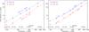 |
Fig. 1 Measurements of the flux density of α Cen A (blue circles) and α Cen B (red circles) with ALMA, with statistical 1σ error bars inside the symbols. Left: assuming that Sν ∝ να, least-square fits to the Bands 3 to 9 flux densities are shown with dashed lines with the power-law exponent α = dlog Sν/ dlog ν shown next to them. Right: fits are shown with solid lines, performed as in the left panel, to the data above, and with dotted lines below 200 GHz (~1.5 mm). The ALMA bands, with their central wavelengths, are identified at the bottom of the figure. |
2. Observations and data reduction
The binary α Cen AB was observed in all six ALMA continuum bands during the period July 2014 to May 2015 (Table 2). The field of view (primary beam) varied from about 10′′ for the shortest wavelength to about 1′ for the longest. Similarly, the angular resolution (synthesized half power beam width) ranged from 02 to 15. With angular diameters of 0008 and 0006 for A and B at 2 μm (Kervella et al. 2003), the stars were point-like to the ALMA interferometer in all wave bands (cf. Table 1). The ALMA program code is 2013.1.00170.S and the observations in Bands 3, 7, and 9 have already been described in detail by Liseau et al. (2015) and are not repeated here.
The observations in Bands 4, 6, and 8 were taken in the standard wideband continuum mode with 8 GHz effective bandwidth spread over four spectral windows in each of the bands. The Band 4 observations, taken on 2015 Jan 18 with 34 antennas, were centered on 145 GHz (2068 μm) with ~24 min of observing time with 5.5 min on source. The Band 6 observations, taken on 2014 Dec 16 with 35 antennas, were centered on 233 GHz (1287 μm) with ~14 min of observing time with ~2 min on source. Finally, the Band 8 observations, taken on 2015 May 2 with 37 antennas, were centered on 405 GHz (740 μm) with ~ 21 min of observing time with ~7 min on source.
The visibilities were flagged and calibrated following standard procedures using the CASA package1 v4.2.2 for Bands 4 and 6, and v4.3.1 for Band 8. The quasar J1617-5848 was used as complex gain calibrator in Bands 4 and 8, while J1408-5712 was used in Band 6. The quasar J1427-4206 was used as bandpass calibrator in Bands 6 and 8, while J1617-5848 was used in Band 4. Flux calibration was carried out with Ceres in Band 4 when at 74° elevation, while α Cen was at 44°. The quasar 1427-421 was used for flux calibration in Band 6 when it was at 57° elevation and α Cen was at 46°, while Titan was used in Band 8 when it was at 50° elevation and α Cen was at 52°.
Imaging was performed using natural weighting in Bands 4, 6, and 8, and one round of phase-only self-calibration was carried out on all three images to improve the rms noise. The synthesized beam sizes are listed in Table 1 and the primary beam-corrected flux densities and the rms noise per synthesized beam in the pointing center are listed in Table 2. We also imaged the ALMA spectral windows separately in each band to assess the spectral index within each band and the resultant flux densities for α Cen A and B are listed in Table A.1.
3. Results
The binary system is well resolved at all frequencies. The J2000-coordinates for α Cen A and B on the observational dates are presented in Table 1, together with the sizes of the synthesized beams (ellipses with semimajor axes a and semiminor axes b in arcseconds) and their orientations (position angle PA in degrees). The frequencies of the bands are given in Table 2, where the primary beam-corrected flux densities, Sν, are reported together with their statistical errors. As can be seen, the signal-to-noise ratio (S/N) spans the range 10–100 for α Cen B, and excels to nearly 300 for α Cen A. The absolute flux calibration is quoted in terms of goals2, viz. better than 5% for bands B 3 and B 4, better than 10% for B 6 and B 7, and at best about 20% for B 8 and B 9. These goals are shown for α Cen A and B in Fig. 2.
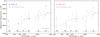 |
Fig. 2 Brightness temperature TB in Kelvin at ALMA wavelengths λ in μm, for Bands 3 to 9 of the G-star α Cen A (left, blue) and the K-star α Cen B (right, red). In addition to the observational rms errors (solid bars), the estimated absolute errors, including calibration uncertaities, are shown as dashed error bars. The stellar photospheres, represented by extrapolations to PHOENIX model atmospheres of Brott & Hauschildt (2005) for the respective stars (Teff, log g, [Fe/H]), and shown as black dashed lines. The ALMA bands are indicated below. A solar model chromosphere (VAL IIIC, Vernazza et al. 1981) is shown as long dashes, with data for the Sun from Loukitcheva et al. (2004) as black open circles. |
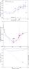 |
Fig. 3 Top: SED of the model chromosphere of the G2 star α Cen A, based on the modified solar C 7 model, is shown with the blue curve. Data are from Spitzer, Herschel, and APEX (Liseau et al. 2013) (small blue symbols and dotted error bars) and from ALMA (big blue squares). The ALMA bands are indicated at the bottom of the figure and the stellar photosphere is shown as RJ(Teff). For comparison, data for the quiet Sun from Loukitcheva et al. (2004) are shown as black open circles. Middle: run of TB with height h with symbols as above. For comparison, also the corresponding model for the K 1 star α Cen B is shown in red, and, for reference, the solar C 7 model as black dots. Bottom: run of density n(H) and turbulent velocity υturb with height h is shown for the solar analog α Cen A. |
Stellar flux ratios and in-band (spw 1 – spw 4) spectral indices.
3.1. Relative fluxes from 0.4 to 3.1 mm
The average flux ratio for the binary over the ALMA bands 3 through 9 is [Sν(B) /Sν(A)] ave = 0.464 ± 0.051 (Table 3). This would be close to the ratio of their respective solid angles (RB/RA)2 = 0.497 ± 0.003, where the radii are those of their interferometrically measured photospheric disks of uniform brightness (Kervella et al. 2003). Comparison with the value for the range 0.09 μm to 70 μm, i.e., 0.44 ± 0.18 (Liseau et al. 2013), indicates an apparently remarkable constancy of the flux ratio over four orders of magnitude in wavelength, from the photospheric emission in the visible to that in the microwave regime.
3.2. Spectral slopes of the SEDs
A first order characterization of the emission mechanism(s) can be obtained from the spectral slope of the logarithmic SED. Assuming that Sν ∝ να, linear regression (Press et al. 1986)3 to the Bands 3 to 9 data results in a spectral index αA, 3−9 = 1.92 ± 1.06 with a χ2 = 0.015 for α Cen A. For α Cen B, the corresponding αB, 3−9 = 1.97 ± 1.50 and χ2 = 0.033; see Fig. 1. The goodness-of-fit is Q = 0.9999 for both.
This apparent constancy of the slope that is close to a value of two over the entire ALMA range, from 0.4 to 3.1 mm, is perhaps surprising. A more careful inspection of the data reveals that the slopes at the shorter wavelengths appear marginally steeper, but that the long-wavelength data, not totally unexpected, seem to flatten out. Dividing the data into two subsets for both stars, i.e., below and above 1.5 mm (200 GHz), yields αA, 34 = 1.4 and αA, 69 = 2.0 for the spectral indices of the α Cen A-SED. Similarly, for α Cen B, αB, 34 = 0.7 and αB, 69 = 2.2 (Fig. 1). In these cases, the formal fit errors are considerably larger for both α Cen A and B. However with regard to the fits in the left panel, the observed Band 3 flux densities are in excess by more than 110σ for A and by more than 30 σ for B. Therefore, the flattening of the SEDs toward lower frequencies is real.
Observations at longer wavelengths would help to better constrain the run of the SED. Unfortunately, at declination south of − 60° the number of sensitive observing facilities is limited. Trigilio et al. (2013) and (2014) proposed Australia Telescope Compact Array (ATCA) observations at 15 mm (17 GHz) and 16 cm (2 GHz). C. Trigilio privately communicated to us that both stars were recently detected at 17 GHz. However, having no further information, we provide here our own flux estimates for ATCA observations of the binary (S/N> 5). These are based on extrapolations beyond ALMA Band 3 and the sensitivity specifications of the 6 km compact array for the K band (15 mm) and C/X band (4 cm)4, resulting in estimates of the S/N = 54 (0.27 mJy) and 13 (0.13 mJy) for α Cen A and S/N = 26 (0.04 mJy) and 7 (0.02 mJy) for α Cen B, respectively. These values refer to 12 hour on-source integrations (rms = 0.003 mJy). The corresponding brightness temperatures are shown below, in Fig. 4.
Spectral indices for flux integrations over the individual bands are shown in Table 3, except for Band 9, where the fractional bandwidth is too small for meaningful measurement, and for Band 7, where the relative errors are too large (negative slope within the band). Inside the individual bands, the data were collected through four spectral windows (spw; see Fig. A.1), with the flux data for these provided in Appendix A.
4. Discussion
4.1. The stellar brightness temperatures
The direct observation of the temperature minima of α Cen AB at far-infrared wavelengths indicated a clear kinship with the Sun’s chromosphere (Liseau et al. 2013, 2015). At these wavelengths, the continuum opacity is dominated by inverse bremsstrahlung, with some contributions due to free-free H− processes (e.g., Dulk 1985; Wedemeyer et al. 2016).
Figure 2 shows the observed SEDs of both stars in terms of their brightness temperatures5![Mathematical equation: \begin{equation} T_{\rm B}(\nu) = \frac { 2\,\pi\,\hbar\,\nu }{ k } \left [\ln \left ( \frac{4\,\pi^2\,R^2_{\rm star}(1.0+h/R_{\rm star})^2\,\hbar\,\nu^3}{D^2\,c^2\,S\!_{\nu}} + 1\right ) \right]^{-1}, \end{equation}](/articles/aa/full_html/2016/10/aa29135-16/aa29135-16-eq104.png) (1)where Rstar is the stellar radius, h is the height at which the observed radiation originates, ν is the radiation frequency, D is the distance to the source, Sν is the observed flux density, and the other symbols have their usual meaning.
(1)where Rstar is the stellar radius, h is the height at which the observed radiation originates, ν is the radiation frequency, D is the distance to the source, Sν is the observed flux density, and the other symbols have their usual meaning.
For the Sun, h/R ~ 10-4, where h refers to the height above the solar photosphere, where the optical depth in the visual τ5000 = 1 and h = 0. We assume similar h/R values for the α Cen stars and use their photospheric radii, i.e., Rstar + h ~ Rstar, where Rstar refers to the values determined by Kervella et al. (2003). When hν/kT ≪ 1 (Rayleigh-Jeans regime), Eq. (2) simplifies to 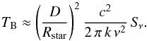 (2)Consequently, in the Rayleigh-Jeans regime (RJ), optically thick free-free emission (or Bremsstrahlung) behaves as Sν ∝ ν2, so that the spectral index, α = Δlog Sν/ Δlog ν = 2 (Fig. 1). In that case, observed brightness temperatures correspond to actual physical temperatures. The data for the α Cen stars reveal a positive temperature gradient that is reminiscent of the solar chromosphere, and different frequencies probe the temperature stratification of the atmosphere. To determine the chromospheric height values h, requires a structure model of the atmosphere that details the run of density and fractional ionization of the gas (De la Luz et al. 2014; Loukitcheva et al. 2015, and references therein).
In Fig. 3, TB(λ) for the disk integrated α Cen A is compared with observed values for the quiet Sun (Loukitcheva et al. 2004).
4.2. Theoretical model chromospheres for α Cen
The region close to the temperature minimum is optically thick in the FIR/submm (Liseau et al. 2015) which, as a consequence of the negative temperature gradient, limits our view to higher, cooler layers above the optical photosphere. Therefore, the received flux at a given frequency directly measures the temperature of the plasma at a particular atmospheric height. This fact can be used to construct analytically the temperature profile to first order and over a limited region (e.g., Liseau et al. 2015, and references therein).
A more sophisticated method is to build a theoretical model chromosphere that at its base is anchored in the photosphere. The result of this is indicated in Fig. 3, showing both the temperature minimum and temperature increase that are retrieved by the semiempirical non-LTE model chromosphere of α Cen A, based on a modified hydrostatic equilibrium model (C7) of the solar chromosphere (Avrett & Loeser 2008; De la Luz et al. 2014). C7 can be viewed as an average of the five most widely used solar chromosphere models (Vernazza et al. 1981; Loukitcheva et al. 2004; Fontenla et al. 2007; Avrett & Loeser 2008; De la Luz et al. 2014).
The temperature profile is computed iteratively from the modified density/pressure structure, ionization balance and opacity (lines and continua). As the conditions in the chromosphere strongly deviate from thermodynamical equilibrium, both the ionization-excitation and the radiative transfer are treated in non-LTE (De la Luz & Tapia, in prep.). Figure 3 also shows the sharp drop in proton density n(H) and the increase of the turbulent speed υturb, steepening into shocks. Although α Cen B is not a solar analog like A, a modified solar model also provides an acceptable fit to the data. The modeled TB(h) of the K-star α Cen B is also shown in Fig. 3.
For α Cen A, the temperature profile is shallower than for the Sun and Tmin = 3548 K at h = 615 km, where the proton density n(H) = 4.7 × 1014 cm-3. The corresponding model parameters for α Cen B are 3407 K, 560 km and 9.5 × 1014 cm-3, respectively.
The temperature minimum in the Teff scale of the α Cen A model, Tmin/Teff = 0.61, is as low as what has been observed in CO lines from the Sun (Tmin/Teff = 0.65; Avrett 2003, and references therein). This is lower than what traditionally has been derived from the wings of resonance lines, viz. > 0.7 for both α Cen A and the Sun (Ayres et al. 1976; Avrett 2003).
Brightness temperatures and chromospheric heights of α Cen A.
At the longest wavelengths, the exponent of the observed SED changes, which is likely because the free-free emission is turning from optically thick to thin beyond 1.5 mm (frequency exponent tends from about 2 to 0). Especially at 3 mm, the Band 3 data are not reproduced well by the model, the density of which is too low to generate sufficient free-free and H− opacity for the required flux. However, from Table 4, it can be seen that the radiation from α Cen A in Bands 4 and 3 probably originates rather high up, at about 2000 km and near the base of the transition region (TR) into the hot corona, which is seen in the X-rays from the α Cen binary (DeWarf et al. 2010; Ayres 2014). The X-ray emission is particularly strong from the more active companion α Cen B.
It is likely that wave energy is dumped and dissipated in these thin layers of the TR base (Soler et al. 2015; Shelyag et al. 2016). Therefore, this region is critical to the understanding of the heating processes of the outer atmospheres of the stars and the Sun. Given the available evidence, ALMA Band 5 observations will eventually be particularly crucial for the observation of these layers in the α Cen stars. These stars deserve continued monitoring, including observations at longer wavelengths.
α Cen A and B are known to be variable on both short and long timescales (DeWarf et al. 2010; Ayres 2015). In X-rays and the FUV, both stars show flickering but also solar-like magnetic cycles, with α Cen B being more active. Repeat observations would assess the level of activity in the submm/mm regime. Between 2014 and 2017, α Cen A is expected to go through its broad shallow maximum of its ~ 19 yr cycle, whereas B presumably passes through a minimum of its 8 year cycle. Thus, perhaps in contrast to the solar case, changes of the chromospheric emission from the active K dwarf could occur over a period of a few years, although such behavior, by analogy with the Sun, would not be expected for the less active α Cen A.
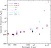 |
Fig. 4 Brightness temperatures for six solar-type stars at wavelengths from 0.5 mm to 6 cm (see the text). Detections were obtained below 1 cm and merely upper limits above that wavelength. The color coding and stellar identifications are given in the upper left corner of the figure. The open circles denote estimates of future ATCA detections of α Cen AB in 12 h at 20 and 6 GHz, respectively (see the text). |
4.3. Comparison with other stars
4.3.1. Solar-type
In addition to α Cen, a handful of other solar-type stars (late F to early K) have been observed at long wavelengths. These stars are all within 6 pc. For ϵ Eridani (K2 V), measurements were made at 1.3 mm and 7 mm (MacGregor et al. 2015) and at 3.6 cm (Güdel 1992) and 6 cm (Bower et al. 2009); for τ Ceti (G8.5 V) at 1.3 mm (MacGregor et al. 2016) and at 8.7 mm and 2 cm (Villadsen et al. 2014). Further, 40 Eridani A (K0.5 V) and η Cassiopeiae A (F9 V) at 8.7 mm, and the latter also at 2 and 6 cm, have also been observed by Villadsen et al. (2014).
As seen in Fig. 4, there is only limited overlap with the wavelength domain of the α Cen binary and upper limits, rather than detections, dominate at cm wavelengths. However, for all detected cases (four stars in addition to α Cen A and B), the fluxes were not consistent with photospheric values but are significantly higher. Therefore, it was generally concluded that this excess emission originates in stellar chromospheres, similar to those in the Sun and α Cen AB.
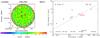 |
Fig. 5 Left: Band 8 observation of α Centauri on 2 May 2015, with the color bar for the intensity shown below. Apart from the well-known binary α Cen A and α Cen B, a previously unknown source U was discovered less than 6′′ north of the primary A. The image is primary beam corrected and the slightly oval synthesized beam (Table 1) is shown in gray in the lower left corner. In the FITS image, the FK5 (J2000.0) coordinates at mid-integration, i.e., JD 2 457 144.632219328, are RA = 14h39m28 |

Primary beam-corrected flux density and 1σ upper limits for the U source in mJy.
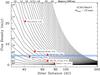 |
Fig. 6 Band 8 flux density as a function of the distance from the Sun with the diameter as the parameter, in 103 km and next to or atop the curves and arbitrarily limited to 6000 km, i.e., slightly smaller than the diameter of Mars. Both the surface temperature and radius are a priori undetermined. A few known TNOs with their names are shown with red dots (www.minorplanetcenter.org/iau/lists/Sizes.html.). In parentheses, the apparent diameter in milli-arcseconds and the estimated blackbody temperature are given. The size of the ALMA synthesized beam, θ = 120 mas, is given in the upper right corner, confirming that these objects would be point-like to ALMA. The observed Band 8 flux density of the unidentified object is indicated by the horizontal blue-shaded dashed line (± 1σ). The distance to the U source remains to be determined. |
4.3.2. Giants
Harper et al. (2013, and references therein) discuss ongoing observational and theoretical work on giants (luminosity class III), and address the possibility of separating the acoustic from MHD heating processes in the upper atmospheres observationally because of the large-scale heights in these stars. Their convective cells and envelopes are much larger than those of main-sequence stars, which may make it possible to distinguish between these effects observationally. In addition and in contrast to the smaller and more compact main-sequence stars (class V), giants are relatively bright and hence offer themselves as possible candidates for calibration purposes for observations in the submm/mm/cm regime (see also Cohen et al. 2005).
4.4. A new, unidentified point-like source near α Cen
In May 2015, an unidentified object was detected in the Band 8 observations of α Cen (Fig. 5). This point source, designated U and with integrated flux over the band of about 4 mJy (Table 5), was within a few arcseconds of the binary. As this object was not detected in any other data set (including UV, VIS and NIR with HST and VLT; see Kervella et al. 2006; Kervella & Thévenin 2007), other epoch data are lacking and hence the nature of this object is unknown.
Figure 5 also shows the SED of this object, consisting of one detection and five upper limits at the 3σ level. However, the data could be consistent with blackbody emission, viz. Sν ∝ ν2, and may be due to a submm galaxy, a stellar object, a brown dwarf or a planetary object. A companion star of the α Cen system does not present a viable explanation, as any star would be brighter than 10th magnitude in the V band, and hence must be discarded.
The submm galaxy option would imply that the proper motion of U would be minuscule, and that it would be quickly left behind the α Cen stars as they pace, at the rate of 37 yr-1, through the sky. As α Cen is in close projection to the plane of the Galaxy, a stellar nature of U may perhaps appear more natural. However, this putative star remained undetected in recent deep searches, implying that U is either a distant heavily extinguished background star or a nearby, very cold object, i.e., a brown dwarf or a planetary object. The parallax and proper motion would clearly distinguish among these possibilities.
Very low-temperature brown dwarves, such as the T 8.5-type ULAS J003402.77−005206.7 with an estimated temperature of 575 K, or the even cooler Y 2 object WISE J085510.83−071442.5 with Teff = 250 K (Tinney et al. 2014; Leggett et al. 2015), can serve as known examples, i.e., an extremely cool brown dwarf at a distance of nearly 20 000 AU may be a viable candidate for the identification of source U. However, like the Y2 object, the Wide-field Infrared Survey Explorer (WISE) should have picked it up. Unless it is close to the very bright α Cen AB, the moderate angular resolution of WISE (>60) presented an obstacle to a clean detection. In the solar system, the projected offset of ~55 would correspond to a distance between Jupiter and Saturn6. However, the identification of U as a planetary companion of α Cen would be totally unrealistic because the observed 740 μm flux would be too high by several orders of magnitude. If U is a body of planetary dimensions, it could possibly be bound to the solar system, but its distance would presently be undetermined. Figure 6 shows the distances and flux densities at 740 μm estimated for several known dwarf planets with the diameter as the parameter. From the figure it is evident that U is likely more distant than Pluto, since a ~1000 km body at roughly 40 AU would have been known for a long time, i.e., for at least ten years. For example, when examining a total of 766 925 known solar-system objects7 for being within 15′ around α Cen at the time of observation, we found no source down to the limiting V magnitude of 26.0. Therefore, a low-albedo, thermal extreme trans-Neptunian object (ETNO), would clearly be consistent with our data (see Fig. 6).
5. Conclusions
ALMA observations of α Centauri at 0.44, 0.74, 0.87, 1.3, 2.1, and 3.1 mm clearly resolved the binary, but not the stellar disks, at all wavelengths. The SEDs of these continuum measurements are consistent with radiation that follows Sν ∝ ν2, except at the lowest frequencies where the SEDs appear to flatten. This is particularly pronounced for the more active secondary, a K 1 star, which is possibly indicative of time variability within half a year or, perhaps more likely, of optically thin free-free emission. The ALMA data were modeled with modified solar chromosphere models that result in the physical structure of the stellar chromospheres. This adapted solar model works very well for the solar analog α Cen A (G2 V), but also for the K1 V star α Cen B. Comparison with the data indicates that the temperature minima of both α Cen A and B are lower than on the quiet Sun. These correspond to the low temperatures seen in lines of the CO molecule on the Sun and occur at atmospheric heights of 615 km and 560 km, respectively. The ALMA data for α Cen AB can be put into context with observations of other nearby solar-type stars that show that chromospheric mm-wave emission is a common feature among these stars and that an increase in the sample size can be expected in the near future.
The ALMA imaging at 0.74 mm led to the discovery of a previously unknown point source within a projected distance of 7.5 AU from α Cen AB. The ALMA observations were performed at different occasions during one year (2014−2015), but this source was clearly detected only on one date. At the three sigma level, the SED of this object is consistent with that of a blackbody and we speculate about its nature. Unless it is a highly variable background source, we find it most likely that it is a distant member of our solar system.
CASA is an acronym for Common Astronomy Software Application.
![Mathematical equation: \hbox{$\chi^2(a,\,b) = \sum_{i=1}^N [(y_i - a -bx_i)/\sigma_i]^2$}](/articles/aa/full_html/2016/10/aa29135-16/aa29135-16-eq181.png) , and
, and  .
.
The brightness temperature, or radiation temperature, is the temperature of a blackbody that emits the same amount of radiation as the observed flux at a given frequency.
The accuracy of the absolute stellar positions will be addressed by Kervella et al. (in prep.).
Acknowledgments
We thank the referee for his/her valuable comments on the manuscript. This paper makes use of the following ALMA data: ADS/JAO.ALMA#2013.1.00170.S. ALMA is a partnership of ESO (representing its member states), NSF (USA), and NINS (Japan), together with NRC (Canada) and NSC and ASIAA (Taiwan), in cooperation with the Republic of Chile. The Joint ALMA Observatory is operated by ESO, AUI/NRAO, and NAOJ.
References
- Avrett, E. H., & Loeser, R. 2008, ApJS, 175, 229 [NASA ADS] [CrossRef] [Google Scholar]
- Avrett, E. H. 2003, in Current Theoretical Models and Future High Resolution Solar Observations: Preparing for ATST, eds. A. A. Pevtsov & H. Uitenbroek, ASP Conf. Ser., 286, 419 [Google Scholar]
- Ayres, T. R. 2014, AJ, 147, 59 [NASA ADS] [CrossRef] [Google Scholar]
- Ayres, T. R. 2015, AJ, 149, 58 [NASA ADS] [CrossRef] [Google Scholar]
- Ayres, T. R., Linsky, J. L., Rodgers, A. W., & Kurucz, R. L. 1976, ApJ, 210, 199 [NASA ADS] [CrossRef] [Google Scholar]
- Bower, G. C., Bolatto, A., Ford, E. B., & Kalas, P. 2009, ApJ, 701, 1922 [NASA ADS] [CrossRef] [Google Scholar]
- Brott, I., & Hauschildt, P. H. 2005, in The Three-Dimensional Universe with Gaia, eds. C. Turon, K. S. O’Flaherty, & M. A. C. Perryman, ESA SP, 576, 565 [Google Scholar]
- Cohen, M., Carbon, D. F., Welch, W. J., et al. 2005, AJ, 129, 2836 [NASA ADS] [CrossRef] [Google Scholar]
- De la Luz, V., Chavez, M., Bertone, E., & Gimenez de Castro, G. 2014, Sol. Phys., 289, 2879 [NASA ADS] [CrossRef] [Google Scholar]
- Demory, B.-O., Ehrenreich, D., Queloz, D., et al. 2015, MNRAS, 450, 2043 [NASA ADS] [CrossRef] [Google Scholar]
- DeWarf, L. E., Datin, K. M., & Guinan, E. F. 2010, ApJ, 722, 343 [NASA ADS] [CrossRef] [Google Scholar]
- Dulk, G. A. 1985, ARA&A, 23, 169 [NASA ADS] [CrossRef] [Google Scholar]
- Dumusque, X., Pepe, F., Lovis, C., et al. 2012, Nature, 491, 207 [NASA ADS] [CrossRef] [PubMed] [Google Scholar]
- Eiroa, C., Marshall, J. P., Mora, A., et al. 2013, A&A, 555, A11 [NASA ADS] [CrossRef] [EDP Sciences] [Google Scholar]
- Fontenla, J. M., Balasubramaniam, K. S., & Harder, J. 2007, ApJ, 667, 1243 [NASA ADS] [CrossRef] [Google Scholar]
- Güdel, M. 1992, A&A, 264, L31 [NASA ADS] [Google Scholar]
- Harper, G. M., O’Riain, N., & Ayres, T. R. 2013, MNRAS, 428, 2064 [NASA ADS] [CrossRef] [Google Scholar]
- Hatzes, A. P. 2013, ApJ, 770, 133 [NASA ADS] [CrossRef] [Google Scholar]
- Kervella, P., & Thévenin, F. 2007, A&A, 464, 373 [NASA ADS] [CrossRef] [EDP Sciences] [Google Scholar]
- Kervella, P., Thévenin, F., Ségransan, D., et al. 2003, A&A, 404, 1087 [NASA ADS] [CrossRef] [EDP Sciences] [Google Scholar]
- Kervella, P., Thévenin, F., Coudé du Foresto, V., & Mignard, F. 2006, A&A, 459, 669 [NASA ADS] [CrossRef] [EDP Sciences] [Google Scholar]
- Leggett, S. K., Morley, C. V., Marley, M. S., & Saumon, D. 2015, ApJ, 799, 37 [NASA ADS] [CrossRef] [Google Scholar]
- Liseau, R., Montesinos, B., Olofsson, G., et al. 2013, A&A, 549, L7 [NASA ADS] [CrossRef] [EDP Sciences] [Google Scholar]
- Liseau, R., Vlemmings, W., Bayo, A., et al. 2015, A&A, 573, L4 [NASA ADS] [CrossRef] [EDP Sciences] [Google Scholar]
- Loukitcheva, M., Solanki, S. K., Carlsson, M., & Stein, R. F. 2004, A&A, 419, 747 [NASA ADS] [CrossRef] [EDP Sciences] [Google Scholar]
- Loukitcheva, M., Solanki, S. K., Carlsson, M., & White, S. M. 2015, A&A, 575, A15 [NASA ADS] [CrossRef] [EDP Sciences] [Google Scholar]
- MacGregor, M. A., Wilner, D. J., Andrews, S. M., Lestrade, J.-F., & Maddison, S. 2015, ApJ, 809, 47 [NASA ADS] [CrossRef] [Google Scholar]
- MacGregor, M. A., Lawler, S. M., Wilner, D. J., et al. 2016, ApJ, 828, 113 [NASA ADS] [CrossRef] [Google Scholar]
- Martí-Vidal, I., Vlemmings, W. H. T., Muller, S., & Casey, S. 2014, A&A, 563, A136 [NASA ADS] [CrossRef] [EDP Sciences] [Google Scholar]
- Press, W. H., Flannery, B. P., & Teukolsky, S. A. 1986, Numerical recipes, The art of scientific computing (CUP) [Google Scholar]
- Rajpaul, V., Aigrain, S., & Roberts, S. 2016, MNRAS, 456, L6 [NASA ADS] [CrossRef] [Google Scholar]
- Shelyag, S., Khomenko, E., de Vicente, A., & Przybylski, D. 2016, ApJ, 819, L11 [NASA ADS] [CrossRef] [Google Scholar]
- Soler, R., Carbonell, M., & Ballester, J. L. 2015, ApJ, 810, 146 [NASA ADS] [CrossRef] [Google Scholar]
- Thévenin, F., Provost, J., Morel, P., et al. 2002, A&A, 392, L9 [NASA ADS] [CrossRef] [EDP Sciences] [Google Scholar]
- Tinney, C. G., Faherty, J. K., Kirkpatrick, J. D., et al. 2014, ApJ, 796, 39 [NASA ADS] [CrossRef] [Google Scholar]
- Torres, G., Andersen, J., & Giménez, A. 2010, A&ARv, 18, 67 [Google Scholar]
- Trigilio, C., Buemi, C., Umana, G., & Leto, P. 2013, Is alpha Centauri revealed by the new generation of radio telescopes?, ATNF Proposal C2836 [Google Scholar]
- Vernazza, J. E., Avrett, E. H., & Loeser, R. 1981, ApJS, 45, 635 [NASA ADS] [CrossRef] [Google Scholar]
- Villadsen, J., Hallinan, G., Bourke, S., Güdel, M., & Rupen, M. 2014, ApJ, 788, 112 [NASA ADS] [CrossRef] [Google Scholar]
- Wang, J., & Fischer, D. A. 2015, AJ, 149, 14 [NASA ADS] [CrossRef] [Google Scholar]
- Wedemeyer, S., Bastian, T., Brajša, R., et al. 2016, Space Sci. Rev., 200, 1 [NASA ADS] [CrossRef] [Google Scholar]
- Wedemeyer-Böhm, S., Steiner, O., Bruls, J., & Rammacher, W. 2007, in The Physics of Chromospheric Plasmas, eds. P. Heinzel, I. Dorotovič, & R. J. Rutten, Heinzel, ASP Conf. Ser., 368 [Google Scholar]
Appendix A: Sub-band fluxes
The flux densities of the spectral windows per band are provided in Table A.1 (α Cen A) and the data are plotted in Fig. A.1. For Band 9, only a single value is given, as the windows are too narrow for meaningful individual measurement.
For α Cen B, the relative drop in intensity in the second spw of Band 4 is conspicuous. This is not evident for α Cen A, and the glitch can therefore not be caused by different calibrations. α Cen AB are point sources and were observed simultaneously. Hence, simultaneous visibility fitting, in which the positions are fixed to reduce the noise (Martí-Vidal et al. 2014), should not result in such large differences unless there is something in the data, e.g., a spectral feature in α Cen B that is not present in the SED of α Cen A. New observations of B, at higher S/N in Band 4, would be necessary to resolve this issue.
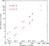 |
Fig. A.1 Measurements of the flux density of α Cen A (blue circles) and of α Cen B (red circles) in the sub-band windows (spw), see Table A.1. The error bars represent the 1σ rms values. Band 9 is too narrow to allow meaningful measurement in sub-windows and only a single value is given. |
Sub-band (spw) flux densities for α Cen AB.
All Tables
Positions of α Cen A and B with ALMA in right ascension and declination (ICRS J 2000.0).
All Figures
|
Fig. 1 Measurements of the flux density of α Cen A (blue circles) and α Cen B (red circles) with ALMA, with statistical 1σ error bars inside the symbols. Left: assuming that Sν ∝ να, least-square fits to the Bands 3 to 9 flux densities are shown with dashed lines with the power-law exponent α = dlog Sν/ dlog ν shown next to them. Right: fits are shown with solid lines, performed as in the left panel, to the data above, and with dotted lines below 200 GHz (~1.5 mm). The ALMA bands, with their central wavelengths, are identified at the bottom of the figure. |
| In the text | |
|
Fig. 2 Brightness temperature TB in Kelvin at ALMA wavelengths λ in μm, for Bands 3 to 9 of the G-star α Cen A (left, blue) and the K-star α Cen B (right, red). In addition to the observational rms errors (solid bars), the estimated absolute errors, including calibration uncertaities, are shown as dashed error bars. The stellar photospheres, represented by extrapolations to PHOENIX model atmospheres of Brott & Hauschildt (2005) for the respective stars (Teff, log g, [Fe/H]), and shown as black dashed lines. The ALMA bands are indicated below. A solar model chromosphere (VAL IIIC, Vernazza et al. 1981) is shown as long dashes, with data for the Sun from Loukitcheva et al. (2004) as black open circles. |
| In the text | |
|
Fig. 3 Top: SED of the model chromosphere of the G2 star α Cen A, based on the modified solar C 7 model, is shown with the blue curve. Data are from Spitzer, Herschel, and APEX (Liseau et al. 2013) (small blue symbols and dotted error bars) and from ALMA (big blue squares). The ALMA bands are indicated at the bottom of the figure and the stellar photosphere is shown as RJ(Teff). For comparison, data for the quiet Sun from Loukitcheva et al. (2004) are shown as black open circles. Middle: run of TB with height h with symbols as above. For comparison, also the corresponding model for the K 1 star α Cen B is shown in red, and, for reference, the solar C 7 model as black dots. Bottom: run of density n(H) and turbulent velocity υturb with height h is shown for the solar analog α Cen A. |
| In the text | |
|
Fig. 4 Brightness temperatures for six solar-type stars at wavelengths from 0.5 mm to 6 cm (see the text). Detections were obtained below 1 cm and merely upper limits above that wavelength. The color coding and stellar identifications are given in the upper left corner of the figure. The open circles denote estimates of future ATCA detections of α Cen AB in 12 h at 20 and 6 GHz, respectively (see the text). |
| In the text | |
|
Fig. 5 Left: Band 8 observation of α Centauri on 2 May 2015, with the color bar for the intensity shown below. Apart from the well-known binary α Cen A and α Cen B, a previously unknown source U was discovered less than 6′′ north of the primary A. The image is primary beam corrected and the slightly oval synthesized beam (Table 1) is shown in gray in the lower left corner. In the FITS image, the FK5 (J2000.0) coordinates at mid-integration, i.e., JD 2 457 144.632219328, are RA = 14h39m28 |
| In the text | |
|
Fig. 6 Band 8 flux density as a function of the distance from the Sun with the diameter as the parameter, in 103 km and next to or atop the curves and arbitrarily limited to 6000 km, i.e., slightly smaller than the diameter of Mars. Both the surface temperature and radius are a priori undetermined. A few known TNOs with their names are shown with red dots (www.minorplanetcenter.org/iau/lists/Sizes.html.). In parentheses, the apparent diameter in milli-arcseconds and the estimated blackbody temperature are given. The size of the ALMA synthesized beam, θ = 120 mas, is given in the upper right corner, confirming that these objects would be point-like to ALMA. The observed Band 8 flux density of the unidentified object is indicated by the horizontal blue-shaded dashed line (± 1σ). The distance to the U source remains to be determined. |
| In the text | |
|
Fig. A.1 Measurements of the flux density of α Cen A (blue circles) and of α Cen B (red circles) in the sub-band windows (spw), see Table A.1. The error bars represent the 1σ rms values. Band 9 is too narrow to allow meaningful measurement in sub-windows and only a single value is given. |
| In the text | |
Current usage metrics show cumulative count of Article Views (full-text article views including HTML views, PDF and ePub downloads, according to the available data) and Abstracts Views on Vision4Press platform.
Data correspond to usage on the plateform after 2015. The current usage metrics is available 48-96 hours after online publication and is updated daily on week days.
Initial download of the metrics may take a while.