| Issue |
A&A
Volume 594, October 2016
|
|
|---|---|---|
| Article Number | A73 | |
| Number of page(s) | 13 | |
| Section | Extragalactic astronomy | |
| DOI | https://doi.org/10.1051/0004-6361/201628711 | |
| Published online | 13 October 2016 | |
Compton-thick AGN in the 70-month Swift-BAT All-Sky Hard X-ray Survey: A Bayesian approach
1 IAASARS, National Observatory of Athens, I. Metaxa & V. Pavlou, 15236 Penteli, Greece
e-mail: aakylas@noa.gr
2 Osservatorio Astronomico di Bologna, INAF, Via Ranzani 1, 40127, Bologna, Italy
Received: 14 April 2016
Accepted: 14 July 2016
The 70-month Swift-BAT catalogue provides a sensitive view of the extragalactic X-ray sky at hard energies (>10 keV) containing about 800 active galactic nuclei (AGN). We explore its content in heavily obscured, Compton-thick AGN by combining the BAT (14−195 keV) with the lower energy XRT (0.3−10 keV) data. We apply a Bayesian methodology using Markov chains to estimate the exact probability distribution of the column density for each source. We find 53 possible Compton-thick sources (probability range 3−100%) translating to a ~7% fraction of the AGN in our sample. We derive the first parametric luminosity function of Compton-thick AGN. The unabsorbed luminosity function can be represented by a double power law with a break at L⋆ ~ 2 × 1042erg s-1 in the 20−40 keV band. The Compton-thick AGN contribute ~17% of the total AGN emissivity. We derive an accurate Compton-thick number count distribution taking into account the exact probability of a source being Compton-thick and the flux uncertainties. This number count distribution is critical for the calibration of the X-ray background synthesis models, i.e. for constraining the intrinsic fraction of Compton-thick AGN. We find that the number counts distribution in the 14−195 keV band agrees well with our models which adopt a low intrinsic fraction of Compton-thick AGN (~ 12%) among the total AGN population and a reflected emission of ~ 5%. In the extreme case of zero reflection, the number counts can be modelled with a fraction of at most 30% Compton-thick AGN of the total AGN population and no reflection. Moreover, we compare our X-ray background synthesis models with the number counts in the softer 2−10 keV band. This band is more sensitive to the reflected component and thus helps us to break the degeneracy between the fraction of Compton-thick AGN and the reflection emission. The number counts in the 2−10 keV band are well above the models which assume a 30% Compton-thick AGN fraction and zero reflection, while they are in better agreement with models assuming 12% Compton-thick fraction and 5% reflection. The only viable alternative for models invoking a high number of Compton-thick AGN is to assume evolution in their number with redshift. For example, in the zero reflection model the intrinsic fraction of Compton-thick AGN should rise from 30% at redshift z ~ 0 to about 50% at a redshift of z = 1.1.
Key words: X-rays: galaxies / surveys / galaxies: Seyfert / quasars: supermassive black holes
© ESO, 2016
1. Introduction
X-ray surveys provide the most efficient way to detect active galactic nuclei (AGN; see Brandt & Alexander 2015 for a recent review). The 4 Ms Chandra Deep Field-South Survey (CDFS) catalog uncovered a surface density of 20,000 AGN/deg2 (Xue et al. 2011), a number which is expected to increase significantly with the additional 3Ms observations to be released within this year. In comparison, optical surveys which detect the most luminous AGN (QSOs) yield surface densities of a few hundred AGN per square degree (Ross et al. 2013). The huge contrast in the efficiency between X-ray and optical surveys lies in the fact that X-ray surveys detect the most highly obscured and low luminosity AGN. The deficit of AGN in optical surveys could only partially be recovered using either variability (Villforth et al. 2010) or emission line ratio diagnostics (Bongiorno et al. 2010). On the other hand, infrared selection techniques, although not affected by obscuration (Stern et al. 2012; Donley et al. 2012; Mateos et al. 2013; Assef et al. 2013), can miss a significant fraction of the less luminous AGN because of contamination by the host galaxy. In conclusion, it is only the X-ray surveys that reliably track the history of accretion into supermassive black holes (SMBH; Ueda et al. 2014; Miyaji et al. 2015; Aird et al. 2015a,b; Ranalli et al. 2016).
Even the extremely efficient X-ray surveys performed by XMM-Newton and Chandra in the 0.3−10 keV band face difficulties when they encounter the most heavily obscured AGN, i.e. those with column densities above 1024cm-2. These are the Compton-thick AGN where the attenuation of X-rays is due to Compton scattering on electrons rather than photoelectric absorption, which is the major attenuation mechanism at lower column densities. The deep Chandra and XMM-Newton surveys found a number of Compton-thick AGN at moderate to high redshift (Comastri et al. 2011; Georgantopoulos et al. 2013; Brightman et al. 2014; Lanzuisi et al. 2015). Harder X-ray (>10 keV) surveys, which are much less prone to obscuration, can yield the least biased samples of Compton-thick AGN compared to any other wavelegth. The Swift (Burst Alert Telescope BAT; Barthelmy 2000) all-sky survey detected a number of heavily obscured AGN at bright fluxes, f14−195 keV ~ 10-11erg cm-2 s-1 (Burlon et al. 2011; Ajello et al. 2012; Ricci et al. 2015) arising from 5−7% of the BAT AGN population. The BAT cannot probe much deeper fluxes because it is a coded-mask detector and thus its spatial resolution is limited. The recently launched NuSTAR mission is carrying the first telescope operating at energies above 10 keV and therefore it can reach a flux limit two orders of magnitude deeper than Swift-BAT before it encounters the confusion limit at about f8−24 keV ~ 10-14 erg cm-2 s-1. The NuSTAR surveys of the COSMOS and the e-CDFS surveys (Civano et al. 2015; and Mullaney et al. 2015, respectively) could yield the first examples of Compton-thick AGN at faint fluxes. However, so far only a few bona fide Compton-thick sources have been detected by NuSTAR owing to its small field of view. Larger numbers will become available when a large number of serendipitous sources have been accumulated.
Despite the scarcity of Compton-thick AGN even in the hard X-ray band, there are two arguments that support the necessity for a large number of these sources.The first argument is the comparison of the X-ray luminosity function with the number density of SMBH in the local Universe first proposed by Soltan (1982). This suggests that a fraction of the SMBH density found in the local Universe cannot be explained by the X-ray luminosity function (Merloni & Heinz 2007; Ueda et al. 2014; Comastri et al. 2015). An explanation for this disagreement is that the accretion is heavily obscured. The second argument has to do with the spectrum of the integrated X-ray light in the Universe, the X-ray background. The X-ray background is mainly due to the X-ray emission from SMBH, but unlike the luminosity function, which is derived from the observed sources, it incorporates the emission from heavily obscured AGN most of which are too faint to be detected even in the deepest X-ray surveys. A number of models have been developed to reconstruct the spectrum of the X-ray background (Comastri et al. 1995; Gilli et al. 2007; Treister et al. 2009; Ballantyne et al. 2011; Akylas et al. 2012; Ueda et al. 2014). All these models require a substantial number of Compton-thick AGN to reproduce the peak of the spectrum between 20 and 30 keV (Marshall et al. 1980; Gruber et al. 1999; Revnivtsev et al. 2003; Frontera et al. 2007; Ajello et al. 2008; Moretti et al. 2009; Türler et al. 2010). However, the exact number is still unconstrained with the various models predicting a fraction of Compton-thick AGN between 10 and 35% of the total AGN population. The most recent X-ray background synthesis models (Treister et al. 2009; Akylas et al. 2012) use the number density of Compton-thick AGN found in the local Universe by Swift-BAT as a calibration. It is therefore important to determine this number precisely.
In this paper, we make use of the 70-month Swift-BAT catalogue in combination with the Swift-XRT, X-ray Telescope (Burrows et al. 2005) to estimate accurate absorbing column densities for all AGN detected in the local Universe in the 14−195 keV energy band. Parallel to our work, Ricci et al. (2015) used exactly the same sample to search for Compton-thick AGN. The present work extends their analysis as we make use of Bayesian statistics to estimate the probability distribution of a source being Compton thick. In addition, using the above Bayesian approach we derive the accurate number count distribution comparing with our X-ray background synthesis models. This comparison derives the intrinsic number of Compton-thick AGN beyond the flux limit of the BAT survey. Finally, we derive the first luminosity function of Compton-thick AGN in the local Universe.
2. X-ray sample
In this work we use the catalogue of sources detected during the 70 months of observations of the BAT hard X-ray detector on board the Swift gamma-ray burst observatory (Baumgartner et al. 2013). The Swift-BAT 70-month survey has detected 1171 hard X-ray sources, more than twice as many sources as the previous 22-month survey in the 14-195 keV band. It is the most sensitive and uniform hard X-ray all-sky survey and reaches a flux level of 1.34 × 10⁻¹¹erg cm-2 s-1 over 90% of the sky. The majority of the sources are AGN, with over 800 in the 70-month survey catalog. In our analysis we consider 688 sources classified according to the NASA/IPAC Extragalactic Database into the following types: (i) 111 galaxies; (ii) 292 Seyfert I (Sy 1.0−1.5); (iii) 262 Seyfert II (Sy 1.7−2.0); and (iv) 23 sources of type “other AGN”. Radio-loud AGN have been excluded since their X-ray emission might be dominated by the jet component. Quasi stellar objects (QSOs) are also excluded from the analysis since the fraction of highly absorbed sources within this population should be negligible.
In order to expand our spectral analysis to lower energies, we combine Swift-BAT data with Swift-XRT observations probing the broad energy range 0.3−195 keV. This allows for the exact determination of the column density. Moreover, the Fe Kα emission line, which is the “smoking gun” of Compton-thick accretion, can be detected. We use the online tool provided by the UK Swift Science Data Centre to build the XRT spectra of the sources listed in the Swift-BAT 70-month catalogue.
The spectra are extracted from all available Swift-XRT observations for any given source. We were able to derive the Swift-XRT spectra for 604 out of 688 sources (88% completeness). For 41 sources in the Seyfert I sample (14%), 23 sources in the Seyfert II sample (9%), 15 sources in the galaxy sample (14%), and 5 sources in the “other AGN” sample (14%) we cannot extract the spectra of the XRT data, mainly because the Swift-XRT observations do not cover the whole sky owing to their smaller field of view with respect to BAT.
3. Spectral fitting
We use XSPEC v12.8.0 (Arnaud 1996) to perform detailed fitting of all 604 spectra in our sample with both XRT and BAT observations available. The fitting is performed in the 0.3−195 keV band using C statistic (Cash 1979) to avoid binning and therefore information loss. For very bright sources with more than 1000 counts, such as NGC 1068 or Circinus, we exclude data below 2 keV to simplify the spectral modelling.
First, we apply an automated procedure to fit all the data using a simple power-law model. A Gaussian line is also included to estimate the strength of the Fe Kα emission line at around 6.4 keV. Since the BAT and the XRT observations are not simultaneous it is possible that some flux variations may appear in the data. We expect these variations to be small because the BAT observations are taken over a long time period and also because the XRT spectra are extracted from all available observations. Therefore, we allow the power-law normalisations within these data-sets to vary freely to account for possible flux variations within a factor of at most two.
The sources that (a) are well fitted by the model (null hypothesis probability >5%); (b) show no evidence for strong emission line (the 3σ upper limit for the equivalent width (EW) Fe Kα is less than 1 keV); (c) the 3σ upper limit for the NH is less than 1024cm-2; and (d) the 3σ limit of the photon index is consistent with the canonical Γ values for AGN (i.e. 1.7−2.0) are considered Compton-thin sources and are excluded from further analysis.
Then we repeat the fitting procedure for the remaining sources using an absorbed double power-law model with tied photon indices plus a Gaussian line. Again, the sources that satisfy all the above criteria are excluded from the sample. This approach removes the majority of the sources (85%) from our sample and reduces the number of Compton-thick candidates to about 70. We fit these most probably highly absorbed sources using the more appropriate torus model described in Brightman & Nandra (2011). We keep the torus opening angle fixed to 60 degrees and the viewing angle to 80 degrees. At this step, along with the standard minimisation algorithm (C-stat) we also adopt a Markov chain Monte Carlo (MCMC) method using the Goodman-Weare algorithm to derive the distribution of the spectral parameters for each source. The idea behind this approach is to assign to each source a probability of being Compton thick and to avoid answering the question (Compton thick or not) based on the best-fit NH and Fe Kα EW values and their confidence intervals.
In total, 53 sources present a non-zero probability of being Compton thick (PCT) that varies from a few per cent up to one hundred per cent. The majority of these sources (41) belong to the Seyfert II class, four sources belong to the Seyfert I class, five sources are in the galaxy class and another four are from the “other AGN” class. In Table A.1 we list the detection and optical counterpart information of the Compton-thick candidates derived from Baumgartner et al. (2013) and address previous references for Compton thickness found in the literature. In Table A.2 we list the most probable Γ and NH values for each source in the Compton-thick candidate sample. We also provide the observed flux and luminosity values in the 2−10 keV, 20−40 keV and 14−195 keV bands.
Taking into account the Compton-thick probability of each source the effective number of Compton-thick sources is ~ 40 sources or ~ 7% of the AGN population in our sample. The 0.3−195 keV count distribution of our sources is plotted in Fig. 1. For clarity, sources with more than 1000 counts are plotted in one bin.
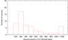 |
Fig. 1 Count distribution in the 0.3−195 keV band for the 53 sources in the Compton-thick sample. For clarity sources with more than 1000 counts appear in one bin in the plot. |
Some examples of the MCMC analysis are presented in Fig. 2 where we plot examples of the source spectrum and its Γ and NH probability distributions derived from the MCMC analysis. In Fig. 3 we plot the average (marginal) Γ and NH distributions for the 53 Compton-thick candidates. To produce these plots we co-added the individual Γ and NH probability distributions derived for each source. A Gaussian function fit to the Γ probability distribution suggests that the peak of the distribution is 1.98 with a standard deviation of 0.2. Furthermore, the NH distribution plot shows that the average probability of a Compton-thick candidate in our sample being a true Compton-thick source is about 80%. The same figure shows that within the Compton-thick population the estimated fraction of reflection dominated sources (NH> 1025 cm-2) is ~10%. The observed ratio, r, of Compton-thick AGN with a column density 1024−1025 cm-2 over those with a column density higher than 1025 cm-2 is 7 ± 3. This is entirely consistent with the ratio obtained by Burlon et al. (2011) considering the very small number statistics, especially in the bin with column densities above 1025 cm-2. However, this observed ratio is biased even in the 14−195 keV band, especially against the sources with column density above 1025 cm-2 and does not represent the intrinsic NH distribution in these bins. The real ratio, after correction for the non-observed sources, is model dependent and can be estimated using our X-ray background models. We find that for the Swift-BAT 70-month survey the observed ratio r is consistent with an intrinsically flat NH distribution (a model with a reflection component of 5% predicts that the observed ratio r is ~4 while the model with a reflection component of 0% predicts that the observed ratio r is ~9).
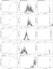 |
Fig. 2 Examples of MCMC simulation results on Compton-thick candidates. Left panel: data and unfolded model fitted. Middle: photon index probability distribution. Right: column density (× 1024 cm-2) probability distribution. |
4. Comparison with previous results
4.1. New Compton-thick sources
First, we discuss the sources with a non-zero probability of being Compton thick based on this work, but without (at least to our knowledge) any previous reference in the literature. There are nine objects (flagged with a “−” symbol in Col. 8 of Table 1). In all the cases the corresponding PCT probability (Col. 4 in Table A.2) ranges from 3% to 70%. Therefore, previous works may not refer to these sources as Compton-thick candidates because the fitting results do not satisfy certain selection criteria, e.g. these sources do not satisfy the criterion of best-fit column density NH> 1024 cm-2 as used in Ricci et al. (2015).
4.2. Conflicting cases
Next, we discuss the two cases that are most likely Compton thick according to our analysis, while conflicting results on their column density are reported in the literature. In particular NGC 4941 and NGC 3081 have probabilities of being Compton-thick 0.75 and 1, respectively. In the case of NGC 4941 Salvati et al. (1997), using BeppoSAX-MECS observations, found a Compton-thick spectrum, with a reflected power law and a large equivalent width iron line. Alternatively, a Compton-thin spectrum, with the intrinsic power law transmitted through a large column density absorber, could provide an acceptable fit to their data. In our analysis, no significant emission line is detected. However, the combined use of XRT and BAT data allow the direct determination of the photoelectric turnover and suggest a probability PCT = 75%. In the case of NGC 3081, Eguchi et al. (2011) analysed Suzaku XISs and the HXD/PIN observations and found a column density of ~ 1024 cm-2. Our results strongly suggest a Compton-thick nucleus with PCT = 1 based on the photo-ionisation turnover. The presence of an Fe Kα with a 3σ upper limit in the equivalent width of ~1.2 keV further suggests the presence of a Compton-thick AGN. Ricci et al. (2015) do not report either of these sources as Compton thick. The spectra of these sources are given in Fig. 4.
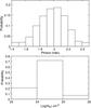 |
Fig. 3 Upper panel: average Γ distribution probability for the 53 Compton-thick candidates. This is the sum of the individual distribution probabilities for each source based on the MCMC. Lower panel: average (marginal) NH distribution probability for the 53 Compton-thick candidates. |
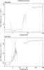 |
Fig. 4 Swift spectra of the sources NGC 4941 and NGC 3081 found as probable Compton thick in this work. |
4.3. Compton-thick sources not confirmed by this work
A thorough review of the literature reveals eight sources in the Swift-BAT catalogue for which there have been claims that these are Compton-thick candidates. Instead, our analysis suggests a zero PCT probability. The spectra of these sources are presented in Fig. 5. In Table 1 we list the best-fitting results. For the analysis we have assumed a double power-law model plus a Gaussian line in order to measure the Fe Kα emission line strength. The errors quoted correspond to the 90% confidence interval.
These sources present an absorbed spectrum with a column density of a few times × 1023 cm-2. The emission line, when present, is fully consistent with the measured NH values. The differences in the estimation of the absorption are usually attributed to variability. For example, Risaliti et al. (2009) has shown that NGC 1365 is a complex source that exhibits NH variability from log NH ≃ 23 to 24 on time scales of 10 h. Similar cases are those of Mrk 1210 and NGC 7582, which are also known for significant changes in the absorbing column density from the Compton-thin to the Compton-thick regime (see e.g. Ohno et al. 2004 and Rivers et al. 2015, respectively).
Ricci et al. (2015) presented combined XMM-Newton and Swift observations of 2MASXJ03502377-5018354 and found evidence that this source is Compton thick with a column density of NH = 2 ± 0.5 × 1024cm-2 and a strong FeKα line (EW ~ 500 eV). Our work instead reveals a highly obscured but not Compton-thick source with  cm-2. However, our analysis is limited by the poor statistics of the XRT spectra. Analysis of the publicly available, high quality NuSTAR observations available (Akylas et al., in prep.) confirm the presence of a high EW Fe line (~ 1 keV) again suggesting that the source is most probably Compton thick.
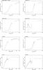 |
Fig. 5 Spectra of the eight sources in our sample previously reported as Compton-thick candidates, with PCT = 0. |
Literature Compton-thick sources not confirmed by this work.
Similarly, in the cases of CGCG420-015 and ESO565-GO19, previously reported as bona fide Compton-thick sources in Severgnini et al. (2011) and Gandhi et al. (2013), our analysis suggests the presence of a high amount of obscuration but clearly below the Compton-thick limit. In these two cases, given the good quality of the XRT data, variability could explain the differences in column density. Moreover, analysis of the publicly available, high quality NuSTAR observations of CGCG420-015 (Akylas et al., in prep.) suggest PCT< 0.5.
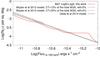 |
Fig. 6 Number count distribution based on the Swift-BAT 70-month survey data (solid line) along with the model predictions of the Akylas et al. (2012) X-ray background synthesis model. Their best-fit model with a Compton-thick fraction of 12% of the total AGN population and a reflected emission of 5% is shown with a dotted line. We also show a model with a Compton-thick fraction of 30% and no reflection (dashed line). Finally, the model of Ueda et al. (2014) is shown with a dot-dashed line. All are in reasonable agreement with the observed number counts |
5. Number count distribution and comparison with models
5.1. Derivation
The MCMC performed in XSPEC provide useful information on the probability of each source being Compton-thick and its flux probability distribution. Using this information we are able to construct the number count distribution for the Compton-thick population without excluding any source from the sample and without the need of a “clean” Compton-thick sample. Following this reasoning, we assign a single PCT probability, which is the probability of being Compton thick, to every source in the sample. We also assign a set of PFlux probabilities, which are the probabilities of finding the source at any given point in the flux space. The product of these two probabilities, corrected for the 70-Month Swift-BAT All-Sky Hard X-ray Survey area curve at the given flux (Baumgartner et al. 2013), gives the weight of each source in the calculation of the number count distribution plot.
As we pointed out earlier, some sources lack XRT data and are excluded from further analysis. However, it is possible that some of these are associated with Compton-thick nuclei. To take this into account, each source excluded from the sample is assigned a probability of being Compton thick. This new probability depends on the ratio of the Compton-thick sources actually found and the total number of sources in a certain class. Therefore, for a missing source in the Seyfert I sample this probability is 1%, for a source in the Seyfert II sample it is 13%, for a source in the galaxy sample it is 4%, and for a source in the “other AGN” sample it is 16%. For all the sources without XRT data, we calculate the 14−195 keV flux fitting only the BAT data with a simple power-law model. Then all 84 sources initially excluded from the analysis are taken into account for the calculation of the number counts distribution with their respective probability of being Compton thick.
In order to estimate the best-fit slope of the number density distribution we use the analytical method proposed in Crawford et al. (1970). We slightly modify this method to account for the survey area curve and the probability of a source being Compton thick. Their result (Eq. (9)) for the slope α of the integral number density distribution (N(S) = kS− α) should be written as  (1)where Ωo is the survey area, Ωi is the survey area for a given source flux, PCT is the probability of a source being Compton thick, and si is the source flux normalised to the minimum flux of the data. Using this expression we find α = 1.38 ± 0.14, where the standard deviation has been obtained from
  (2)
(2)
5.2. Comparison with X-ray background synthesis models
In Fig. 6 we plot our results. The number count distribution for the Compton-thick sources in the 14−195 keV band is shown with the solid line. The dotted line denotes the model predictions on the number count distribution based on the Akylas et al. (2012) best-fit model for the X-ray background synthesis; this assumes a Compton-thick fraction of 12% of the total AGN population and 5% reflected emission (i.e. reflected emission accounts for 5% of the unabsorbed 2−10 keV luminosity). The observed number count distribution is consistent with this model. The fraction of Compton-thick sources sensitively depends on the amount of reflected emission around the nucleus in the sense that the higher the reflected emission, the lower the fraction of Compton-thick sources. Assuming no reflection, the fraction of Compton-thick sources should increase to 30% of the AGN population in order to be in agreement with the observed counts. Although the latter model provides an equally good representation of the number counts in the 14−195 keV band, we note that it does not provide an acceptable fit to the X-ray background spectrum (see Fig. 2 of Akylas et al. 2012). In the same figure we make a comparison with the model of Ueda et al. (2014). This model uses a large fraction of Compton-thick AGN (~50% of the obscured AGN population) and a moderate amount of reflection. However, an additional feature of this model is that the fraction of the Compton-thick AGN increases with redshift. This model is also in good agreement with the observed number counts.
Additional constraints on the fraction of Compton-thick sources can be provided in the 2−10 keV band. This softer band is largely affected by the reflection component thus helping to break the degeneracy between the fraction of Compton-thick sources and the reflection. In Fig. 7 we plot the number count distribution of the Compton-thick sources in the 2−10 keV band from the XMM-Newton analysis of Lanzuisi et al. (2015) in the COSMOS field and compare it with our models. The number count distribution for the Compton-thick sources is shown with crosses. The model with a Compton-thick fraction of 30% and no reflection falls well below the observed 2−10 keV number counts. The dotted line denotes the model predictions based on the best-fit model of Akylas et al. (2012), i.e. a Compton-thick fraction of 12% of the total AGN population and 5% reflected emission. This model appears to provide a better fit to the 2−10 keV number counts. The model of Ueda et al. (2014) is also plotted. This model falls below the observed counts at bright fluxes, but it starts to agree with the data at fainter fluxes. Although not plotted here, we note that a fraction of Compton-thick AGN as high as 50% (assuming no reflection) can bring the Akylas et al. (2012) models into agreement with the observed counts in the 2−10 keV band. Such a high fraction of Compton-thick AGN would be in rough agreement with the analysis of Buchner et al. (2015). Therefore, the only way to bring a model which assumes a high fraction of Compton-thick AGN into agreement with the number counts in both the 14−195 and the 2−10 keV bands is to assume an evolution of the number density of Compton-thick AGN. Considering the zero reflection model this evolution should increase the fraction of Compton-thick AGN from 30% at a redshift of z ~ 0 (the average redshift of the Swift-BAT Compton-thick AGN) to about 50% at z ~ 1.1 (the redshift of the XMM-Newton Compton-thick AGN).
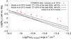 |
Fig. 7 Number count distribution in the 2−10 keV band from the XMM-Newton analysis of Lanzuisi et al. (2015) in the COSMOS field (shown as crosses) compared with the model predictions of the Akylas et al. (2012) model. Their best-fit model with a Compton-thick fraction of 12% of the total AGN population and a reflected emission of 5% is shown with a dotted line. We also show a model with a Compton-thick fraction of 30% and no reflection (dashed line). The model of Ueda et al. (2014) is also shown for comparison. |
6. Luminosity function
A binned luminosity function (LF) is essentially Φ(L,z) ~ N/V, where L and z are the average luminosity and redshift of the bin, respectively; N is the number of objects in the bin; and V is the comoving volume probed by the survey in the bin (see Eqs. (5) and (6) in Lanzuisi et al. 2015; Marshall et al. 1980; Ranalli et al. 2016). Weighting of sources can be introduced in a binned LF by replacing the number of objects N with the sum of weights wi of each source i: N ~ ∑ iwi (see e.g. Liu et al. 2008). We show the binned LF in Fig. 8 for eight bins of luminosity spanning the 1041–1044.5 erg s-1 range. We only consider one bin in redshift, 0.0001 ≤ z ≤ 0.15. We also present a parametric estimate of the LF. We consider a double power-law form (Maccacaro et al. 1984; Ranalli et al. 2016). On the same figure we present the Swift-BAT Compton-thin AGN LF derived from Ajello et al. (2012) (magenta dash-dotted line) and the NuSTAR AGN LF derived by Aird et al. (2015b) (green crosses) ![\begin{equation} \label{eq:doublepow} \frac{\Phi (L)}{ \log L} = A \left[ \left( \frac{L}{L_*} \right)^{\gamma_1} + \left( \frac{L}{L_*} \right)^{\gamma_2} \right]^{-1} , \end{equation}](/articles/aa/full_html/2016/10/aa28711-16/aa28711-16-eq95.png) (3)where A is the normalisation, L∗ is the knee luminosity, and γ1 and γ2 are the slopes of the power-law below and above L∗.
(3)where A is the normalisation, L∗ is the knee luminosity, and γ1 and γ2 are the slopes of the power-law below and above L∗.
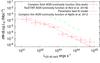 |
Fig. 8 Compton-thick AGN luminosity function in the 20−40 keV band derived from our sample; the binned luminosity function is denoted with red points and the parametric with the red line. The magenta dash-dotted line denotes the Compton-thin AGN luminosity function derived by Ajello et al. (2012). The green points show the NuSTAR AGN luminosity function derived by Aird et al. (2015b). |
Parametric fits are usually done by maximising the likelihood of the data under the model. A likelihood function for a LF has been introduced by Marshall et al. (1980) and Loredo (2004). It is based on the Poissonian probability of detecting a number yi of AGN of given luminosity Li and redshift zi, 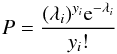 (4)with
 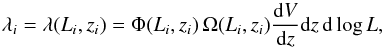 (5)where λ is the expected number of AGN with given Li and zi, and Φ is the LF evaluated at Li and zi. If the (L,z) space is ideally divided into cells that are small enough to contain at most one AGN, then yi = 1 when the cell contains one AGN, and yi = 0 otherwise. The likelihood is therefore the product of the Poissonian probabilities for all cells. This is the reasoning followed by both Marshall et al. (1980) and Loredo (2004).
However, we want to weight the Compton-thick AGN according to their probability. Therefore, we need to allow yi = wi, with 0 ≤ wi ≤ 1. The Poisson distribution is only defined for discrete yi, but it can be extended to the continuous case by replacing the factorial with the Γ function, 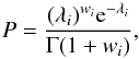 (6)therefore, the likelihood is (compare with Eq. (20) in Ranalli et al. 2016)
 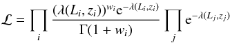 (7)and the log-likelihood S = ln ℒ may be written as (compare with Eq. (22) in Ranalli et al. 2016)
 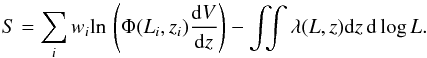 (8)We consider no evolution because of the short redshift interval spanned by our sources. The best-fit parameters are A = 5.5 × 10⁻⁵ Mpc-3, γ1 = 0.30, γ2 = 1.56, and L∗ = 1.4 × 1042 erg s-1. Based on this luminosity function we derive a Compton-thick emissivity (luminosity density) of 7.7 × 1037erg s-1 Mpc-3 in the 20−40 keV band. As the total AGN emissivity is 4.5 × 1038erg s-1 Mpc-3, as derived from the total AGN luminosity function (Ajello et al. 2012), the Compton-thick contribution to the total AGN emissivity is about 17%.
7. Summary
We explore the X-ray spectral properties of AGN selected from the 70-month Swift-BAT all-sky survey in the 14−195 keV band to constrain the number of Compton-thick sources in the local universe. We combine the BAT with the XRT data (0.3−10 keV) at softer energies adopting a Bayesian approach to fit the data using Markov chains. This allows us to consider all sources as potential Compton-thick candidates at a certain level of probability. The probability ranges from 0.03 for marginally Compton-thick sources to 1 for the bona fide Compton-thick cases. The important characteristic of this approach is that intermediate sources, i.e. sources whose column densities lie on the Compton-thick boundary, are assigned a certain weight based on a solid statistical basis.
Based on our analysis, 53 sources in the Swift-BAT catalogue present a non-zero probability of being Compton-thick corresponding to 40 “effective” Compton-thick sources. These sources represent ~7% of the sample in reasonable agreement with the figures quoted in Ricci et al. (2015) and Burlon et al. (2011). We use the same approach to derive the Compton-thick luminosity function in the 20−40 keV band. This can be represented by a double power law with a break luminosity at L⋆ ≈ 1.4 × 1042erg s-1. The Compton-thick AGN contribute 17% of the total AGN emissivity in the 20−40 keV band where the X-ray background energy density peaks.
We compare this log N-log S with our X-ray background synthesis models (Akylas et al. 2012). The main aim of this comparison is to constrain the intrinsic fraction of Compton-thick AGN. In all X-ray background synthesis models, there is a close dependence of the fraction of Compton-thick AGN on the amount of reflected emission close to the nucleus. Assuming 5% reflected emission, we find that the Compton-thick fraction is ~15% of the obscured AGN population (or 12% of the total AGN population). Alternatively, a 30% Compton-thick AGN fraction (with no reflected emission) provides an equally good fit to the 14−195 keV number counts. This can be considered as the upper limit on the fraction of Compton-thick AGN. In addition, we compare the above models with the number count distribution in the 2−10 keV band as this band is more sensitive to the amount of reflected emission. Therefore, this comparison could help us to break the degeneracy between the amount of reflected emission and the fraction of Compton-thick AGN. We compare our model with the XMM-Newton COSMOS field results by Lanzuisi et al. (2015). A 12% Compton-thick fraction (among the total AGN population) with 5% reflection provides a good fit to the data, while the 30% Compton-thick fraction model falls well below the data. Instead, a model with a 50% Compton-thick AGN fraction would be in agreement with the 2−10 keV number counts. An alternative possibility is that there is evolution in the number of Compton-thick AGN between z ~ 0 and z ~ 1.1 (the average redshift) of the COSMOS Compton-thick AGN. Such a strong evolution of the number of Compton-thick AGN is along the lines of the luminosity function models of Ueda et al. (2014).
Most X-ray background synthesis models involve Compton-thick AGN with intrinsic luminosities of the order L2−10 keV) > 1042erg s-1. However, it is likely that there is a large number of Compton-thick AGN which are too faint and remain undetected even in the deepest Chandra surveys. This is the often called “bottom of the barrel” of Compton-thick AGN. For example, Risaliti et al. (1999) found that optically [OIII] selected Compton-thick AGN form at least 50% of the obscured AGN population. These AGN may not contribute significantly to the spectrum of the X-ray background owing to their faint luminosities. However, these AGN could form a substantial fraction of the black hole mass density in the Universe (Comastri et al. 2015).
Acknowledgments
We thank the referee Prof. C. Done for many useful suggestions. We thank Prof. Y. Ueda for providing us with his X-ray background synthesis model predictions. We also thank Dr. Claudio Ricci for his comments. This work is based on observations obtained with XMM-Newton, an ESA science mission with instruments and contributions directly funded by ESA Member States and the USA (NASA).
References
- Aird, J., Alexander, D. M., Ballantyne, D. R., et al. 2015a, ApJ, 815, 66 [NASA ADS] [CrossRef] [Google Scholar]
- Aird, J., Coil, A. L., Georgakakis, A., et al. 2015b, MNRAS, 451, 1892 [NASA ADS] [CrossRef] [Google Scholar]
- Ajello, M., Greiner, J., Sato, G., et al. 2008, ApJ, 689, 666 [NASA ADS] [CrossRef] [Google Scholar]
- Ajello, M., Alexander, D. M., Greiner, J., et al. 2012, ApJ, 749, 21 [NASA ADS] [CrossRef] [Google Scholar]
- Akylas, A., Georgakakis, A., Georgantopoulos, I., Brightman, M., & Nandra, K. 2012, A&A, 546, A98 [NASA ADS] [CrossRef] [EDP Sciences] [Google Scholar]
- Annuar, A., Gandhi, P., Alexander, D. M., et al. 2015, ApJ, 815, 36 [NASA ADS] [CrossRef] [Google Scholar]
- Arévalo, P., Bauer, F. E., Puccetti, S., et al. 2014, ApJ, 791, 81 [NASA ADS] [CrossRef] [Google Scholar]
- Arnaud, K. A. 1996, in Astronomical Data Analysis Software and Systems V, eds. G. H. Jacoby, & J. Barnes, ASP Conf. Ser., 101, 17 [Google Scholar]
- Assef, R. J., Stern, D., Kochanek, C. S., et al. 2013, ApJ, 772, 26 [NASA ADS] [CrossRef] [Google Scholar]
- Ballantyne, D. R., Draper, A. R., Madsen, K. K., Rigby, J. R., & Treister, E. 2011, ApJ, 736, 56 [NASA ADS] [CrossRef] [Google Scholar]
- Baloković, M., Comastri, A., Harrison, F. A., et al. 2014, ApJ, 794, 111 [NASA ADS] [CrossRef] [Google Scholar]
- Barthelmy, S. D. 2000, in X-ray and Gamma-ray Instrumentation for Astronomy XI, eds. K. A. Flanagan, & O. H. Siegmund, Proc. SPIE, 4140, 50 [Google Scholar]
- Baumgartner, W. H., Tueller, J., Markwardt, C. B., et al. 2013, ApJS, 207, 19 [NASA ADS] [CrossRef] [EDP Sciences] [Google Scholar]
- Bongiorno, A., Mignoli, M., Zamorani, G., et al. 2010, A&A, 510, A56 [NASA ADS] [CrossRef] [EDP Sciences] [Google Scholar]
- Brandt, W. N., & Alexander, D. M. 2015, A&ARv, 23, 1 [Google Scholar]
- Brightman, M., & Nandra, K. 2011, MNRAS, 413, 1206 [CrossRef] [Google Scholar]
- Brightman, M., Nandra, K., Salvato, M., et al. 2014, MNRAS, 443, 1999 [NASA ADS] [CrossRef] [Google Scholar]
- Buchner, J., Georgakakis, A., Nandra, K., et al. 2015, ApJ, 802, 89 [NASA ADS] [CrossRef] [Google Scholar]
- Burlon, D., Ajello, M., Greiner, J., et al. 2011, ApJ, 728, 58 [NASA ADS] [CrossRef] [Google Scholar]
- Burrows, D. N., Hill, J. E., Nousek, J. A., et al. 2005, Space Sci. Rev., 120, 165 [NASA ADS] [CrossRef] [Google Scholar]
- Burtscher, L., Orban de Xivry, G., Davies, R. I., et al. 2015, A&A, 578, A47 [NASA ADS] [CrossRef] [EDP Sciences] [Google Scholar]
- Cash, W. 1979, ApJ, 228, 939 [NASA ADS] [CrossRef] [Google Scholar]
- Civano, F., Hickox, R. C., Puccetti, S., et al. 2015, ApJ, 808, 185 [NASA ADS] [CrossRef] [Google Scholar]
- Comastri, A., Setti, G., Zamorani, G., & Hasinger, G. 1995, A&A, 296, 1 [NASA ADS] [Google Scholar]
- Comastri, A., Iwasawa, K., Gilli, R., et al. 2010, ApJ, 717, 787 [NASA ADS] [CrossRef] [Google Scholar]
- Comastri, A., Ranalli, P., Iwasawa, K., et al. 2011, A&A, 526, L9 [NASA ADS] [CrossRef] [EDP Sciences] [Google Scholar]
- Comastri, A., Gilli, R., Marconi, A., Risaliti, G., & Salvati, M. 2015, A&A, 574, L10 [NASA ADS] [CrossRef] [EDP Sciences] [Google Scholar]
- Crawford, D. F., Jauncey, D. L., & Murdoch, H. S. 1970, ApJ, 162, 405 [NASA ADS] [CrossRef] [Google Scholar]
- Donley, J. L., Koekemoer, A. M., Brusa, M., et al. 2012, ApJ, 748, 142 [NASA ADS] [CrossRef] [Google Scholar]
- Eguchi, S., Ueda, Y., Awaki, H., et al. 2011, ApJ, 729, 31 [NASA ADS] [CrossRef] [Google Scholar]
- Frontera, F., Orlandini, M., Landi, R., et al. 2007, ApJ, 666, 86 [NASA ADS] [CrossRef] [Google Scholar]
- Gandhi, P., Terashima, Y., Yamada, S., et al. 2013, ApJ, 773, 51 [NASA ADS] [CrossRef] [Google Scholar]
- Georgantopoulos, I., Rovilos, E., Akylas, A., et al. 2011, A&A, 534, A23 [NASA ADS] [CrossRef] [EDP Sciences] [Google Scholar]
- Georgantopoulos, I., Comastri, A., Vignali, C., et al. 2013, A&A, 555, A43 [NASA ADS] [CrossRef] [EDP Sciences] [Google Scholar]
- Gilli, R., Comastri, A., & Hasinger, G. 2007, A&A, 463, 79 [NASA ADS] [CrossRef] [EDP Sciences] [Google Scholar]
- González-Martín, O., Masegosa, J., Márquez, I., & Guainazzi, M. 2009, ApJ, 704, 1570 [NASA ADS] [CrossRef] [Google Scholar]
- González-Martín, O., Papadakis, I., Braito, V., et al. 2011, A&A, 527, A142 [NASA ADS] [CrossRef] [EDP Sciences] [Google Scholar]
- Greenhill, L. J., Tilak, A., & Madejski, G. 2008, ApJ, 686, L13 [NASA ADS] [CrossRef] [Google Scholar]
- Gruber, D. E., Matteson, J. L., Peterson, L. E., & Jung, G. V. 1999, ApJ, 520, 124 [NASA ADS] [CrossRef] [Google Scholar]
- Hernández-García, L., Masegosa, J., González-Martín, O., & Márquez, I. 2015, A&A, 579, A90 [NASA ADS] [CrossRef] [EDP Sciences] [Google Scholar]
- Koss, M. J., Romero-Cañizales, C., Baronchelli, L., et al. 2015, ApJ, 807, 149 [NASA ADS] [CrossRef] [Google Scholar]
- Lanzuisi, G., Ranalli, P., Georgantopoulos, I., et al. 2015, A&A, 573, A137 [NASA ADS] [CrossRef] [EDP Sciences] [Google Scholar]
- Liu, C. T., Capak, P., Mobasher, B., et al. 2008, ApJ, 672, 198 [NASA ADS] [CrossRef] [Google Scholar]
- Loredo, T. J. 2004, in AIP Conf. Ser. 735, eds. R. Fischer, R. Preuss, & U. V. Toussaint, 195 [Google Scholar]
- Maccacaro, T., Gioia, I. M., & Stocke, J. T. 1984, ApJ, 283, 486 [NASA ADS] [CrossRef] [Google Scholar]
- Maiolino, R., Salvati, M., Bassani, L., et al. 1998, A&A, 338, 781 [NASA ADS] [Google Scholar]
- Malizia, A., Bassani, L., Panessa, F., de Rosa, A., & Bird, A. J. 2009, MNRAS, 394, L121 [NASA ADS] [CrossRef] [Google Scholar]
- Marinucci, A., Bianchi, S., Matt, G., et al. 2016, MNRAS, 456, L94 [NASA ADS] [CrossRef] [Google Scholar]
- Marshall, F. E., Boldt, E. A., Holt, S. S., et al. 1980, ApJ, 235, 4 [NASA ADS] [CrossRef] [Google Scholar]
- Mateos, S., Alonso-Herrero, A., Carrera, F. J., et al. 2013, MNRAS, 434, 941 [NASA ADS] [CrossRef] [Google Scholar]
- Merloni, A., & Heinz, S. 2007, MNRAS, 381, 589 [NASA ADS] [CrossRef] [Google Scholar]
- Miyaji, T., Hasinger, G., Salvato, M., et al. 2015, ApJ, 804, 104 [NASA ADS] [CrossRef] [Google Scholar]
- Moretti, A., Pagani, C., Cusumano, G., et al. 2009, A&A, 493, 501 [NASA ADS] [CrossRef] [EDP Sciences] [Google Scholar]
- Mullaney, J. R., Del-Moro, A., Aird, J., et al. 2015, ApJ, 808, 185 [Google Scholar]
- Ohno, M., Fukazawa, Y., & Iyomoto, N. 2004, PASJ, 56, 425 [NASA ADS] [CrossRef] [Google Scholar]
- Puccetti, S., Comastri, A., Fiore, F., et al. 2014, ApJ, 793, 26 [NASA ADS] [CrossRef] [Google Scholar]
- Puccetti, S., Comastri, A., Bauer, F. E., et al. 2016, A&A, 585, A157 [NASA ADS] [CrossRef] [EDP Sciences] [Google Scholar]
- Ranalli, P., Koulouridis, E., Georgantopoulos, I., et al. 2016, A&A, 590, A80 [NASA ADS] [CrossRef] [EDP Sciences] [Google Scholar]
- Revnivtsev, M., Gilfanov, M., Sunyaev, R., Jahoda, K., & Markwardt, C. 2003, A&A, 411, 329 [NASA ADS] [CrossRef] [EDP Sciences] [Google Scholar]
- Ricci, C., Ueda, Y., Koss, M. J., et al. 2015, ApJ, 815, L13 [NASA ADS] [CrossRef] [Google Scholar]
- Ricci, C., Bauer, F. E., Arevalo, P., et al. 2016, ApJ, 820, 5 [NASA ADS] [CrossRef] [Google Scholar]
- Risaliti, G., Maiolino, R., & Salvati, M. 1999, ApJ, 522, 157 [NASA ADS] [CrossRef] [Google Scholar]
- Risaliti, G., Salvati, M., Elvis, M., et al. 2009, MNRAS, 393, L1 [NASA ADS] [CrossRef] [Google Scholar]
- Rivers, E., Baloković, M., Arévalo, P., et al. 2015, ApJ, 815, 55 [NASA ADS] [CrossRef] [Google Scholar]
- Ross, N. P., McGreer, I. D., White, M., et al. 2013, ApJ, 773, 14 [NASA ADS] [CrossRef] [Google Scholar]
- Salvati, M., Bassani, L., della Ceca, R., et al. 1997, A&A, 323, L1 [NASA ADS] [Google Scholar]
- Severgnini, P., Caccianiga, A., Della Ceca, R., et al. 2011, A&A, 525, A38 [NASA ADS] [CrossRef] [EDP Sciences] [Google Scholar]
- Soltan, A. 1982, MNRAS, 200, 115 [NASA ADS] [CrossRef] [Google Scholar]
- Stern, D., Assef, R. J., Benford, D. J., et al. 2012, ApJ, 753, 30 [NASA ADS] [CrossRef] [Google Scholar]
- Treister, E., Urry, C. M., & Virani, S. 2009, ApJ, 696, 110 [NASA ADS] [CrossRef] [Google Scholar]
- Türler, M., Chernyakova, M., Courvoisier, T. J.-L., et al. 2010, A&A, 512, A49 [NASA ADS] [CrossRef] [EDP Sciences] [Google Scholar]
- Ueda, Y., Eguchi, S., Terashima, Y., et al. 2007, ApJ, 664, L79 [NASA ADS] [CrossRef] [Google Scholar]
- Ueda, Y., Akiyama, M., Hasinger, G., Miyaji, T., & Watson, M. G. 2014, ApJ, 786, 104 [NASA ADS] [CrossRef] [Google Scholar]
- Villforth, C., Koekemoer, A. M., & Grogin, N. A. 2010, ApJ, 723, 737 [NASA ADS] [CrossRef] [Google Scholar]
- Xue, Y. Q., Luo, B., Brandt, W. N., et al. 2011, ApJS, 195, 10 [NASA ADS] [CrossRef] [Google Scholar]
Appendix A: Additional tables
Detection and optical counterpart information of Compton-thick candidates from Baumgartner et al. (2013).
MCMC fitting results for the Compton-thick sample.
All Tables
Detection and optical counterpart information of Compton-thick candidates from Baumgartner et al. (2013).
All Figures
|
Fig. 1 Count distribution in the 0.3−195 keV band for the 53 sources in the Compton-thick sample. For clarity sources with more than 1000 counts appear in one bin in the plot. |
| In the text | |
|
Fig. 2 Examples of MCMC simulation results on Compton-thick candidates. Left panel: data and unfolded model fitted. Middle: photon index probability distribution. Right: column density (× 1024 cm-2) probability distribution. |
| In the text | |
|
Fig. 3 Upper panel: average Γ distribution probability for the 53 Compton-thick candidates. This is the sum of the individual distribution probabilities for each source based on the MCMC. Lower panel: average (marginal) NH distribution probability for the 53 Compton-thick candidates. |
| In the text | |
|
Fig. 4 Swift spectra of the sources NGC 4941 and NGC 3081 found as probable Compton thick in this work. |
| In the text | |
|
Fig. 5 Spectra of the eight sources in our sample previously reported as Compton-thick candidates, with PCT = 0. |
| In the text | |
|
Fig. 6 Number count distribution based on the Swift-BAT 70-month survey data (solid line) along with the model predictions of the Akylas et al. (2012) X-ray background synthesis model. Their best-fit model with a Compton-thick fraction of 12% of the total AGN population and a reflected emission of 5% is shown with a dotted line. We also show a model with a Compton-thick fraction of 30% and no reflection (dashed line). Finally, the model of Ueda et al. (2014) is shown with a dot-dashed line. All are in reasonable agreement with the observed number counts |
| In the text | |
|
Fig. 7 Number count distribution in the 2−10 keV band from the XMM-Newton analysis of Lanzuisi et al. (2015) in the COSMOS field (shown as crosses) compared with the model predictions of the Akylas et al. (2012) model. Their best-fit model with a Compton-thick fraction of 12% of the total AGN population and a reflected emission of 5% is shown with a dotted line. We also show a model with a Compton-thick fraction of 30% and no reflection (dashed line). The model of Ueda et al. (2014) is also shown for comparison. |
| In the text | |
|
Fig. 8 Compton-thick AGN luminosity function in the 20−40 keV band derived from our sample; the binned luminosity function is denoted with red points and the parametric with the red line. The magenta dash-dotted line denotes the Compton-thin AGN luminosity function derived by Ajello et al. (2012). The green points show the NuSTAR AGN luminosity function derived by Aird et al. (2015b). |
| In the text | |
Current usage metrics show cumulative count of Article Views (full-text article views including HTML views, PDF and ePub downloads, according to the available data) and Abstracts Views on Vision4Press platform.
Data correspond to usage on the plateform after 2015. The current usage metrics is available 48-96 hours after online publication and is updated daily on week days.
Initial download of the metrics may take a while.