| Issue |
A&A
Volume 594, October 2016
|
|
|---|---|---|
| Article Number | A34 | |
| Number of page(s) | 9 | |
| Section | Extragalactic astronomy | |
| DOI | https://doi.org/10.1051/0004-6361/201527876 | |
| Published online | 06 October 2016 | |
Detailed photometric analysis of young star groups in the galaxy NGC 300⋆
1 Instituto de Astrofísica de La Plata (CONICET-UNLP), Paseo del bosque S/N, La Plata (B1900FWA), Argentina
e-mail: This email address is being protected from spambots. You need JavaScript enabled to view it.
2 Facultad de Ciencias Astronómicas y Geofísicas, Universidad Nacional de La Plata, Paseo del bosque S/N, La Plata (B1900FWA), Argentina
Received: 2 December 2015
Accepted: 10 August 2016
Abstract
Aims. The purpose of this work is to understand the global characteristics of the stellar populations in NGC 300. In particular, we focused our attention on searching young star groups and study their hierarchical organization. The proximity and orientation of this Sculptor Group galaxy make it an ideal candidate for this study.
Methods. The research was conducted using archival point spread function (PSF) fitting photometry measured from images in multiple bands obtained with the Advanced Camera for Surveys of the Hubble Space Telescope (ACS/HST). Using the path linkage criterion (PLC), we cataloged young star groups and analyzed them from the observation of individual stars in the galaxy NGC 300. We also built stellar density maps from the bluest stars and applied the SExtractor code to identify overdensities. This method provided an additional tool for the detection of young stellar structures. By plotting isocontours over the density maps and comparing the two methods, we could infer and delineate the hierarchical structure of the blue population in the galaxy. For each region of a detected young star group, we estimated the size and derived the radial surface density profiles for stellar populations of different color (blue and red). A statistical decontamination of field stars was performed for each region. In this way it was possible to build the color–magnitude diagrams (CMD) and compare them with theoretical evolutionary models. We also constrained the present-day mass function (PDMF) per group by estimating a value for its slope.
Results. The blue population distribution in NGC 300 clearly follows the spiral arms of the galaxy, showing a hierarchical behavior in which the larger and loosely distributed structures split into more compact and denser ones over several density levels. We created a catalog of 1147 young star groups in six fields of the galaxy NGC 300, in which we present their fundamental characteristics. The mean and the mode radius values obtained from the size distribution are both 25 pc, in agreement with the value for the Local Group and nearby galaxies. Additionally, we found an average PDMF slope that is compatible with the Salpeter value.
Key words: stars: luminosity function, mass function / galaxies: individual: NGC 300 / galaxies: star clusters: general / galaxies: star formation
Full Table 2 is only available at the CDS via anonymous ftp to cdsarc.u-strasbg.fr (130.79.128.5) or via http://cdsarc.u-strasbg.fr/viz-bin/qcat?J/A+A/594/A34
© ESO, 2016
1. Introduction
The distribution and properties of stellar clusters and star-forming complexes provide valuable information that helps understanding the history of the star formation inside galaxies and the way this is related with the dynamic and chemical enrichment of each system. This reveals the importance of performing global studies and assembling catalogs of clusters over the nearest galaxies.
The galaxy NGC 300 is the brightest of five main spiral galaxies forming the Sculptor Group. It is a spiral galaxy Sc D (McConnachie 2012) and presents several regions of massive star formation. This galaxy also has an orientation that minimizes the absorption effects, and it is located close enough to identify stellar clusters and their individual members by using images from telescopes with excellent angular resolution. In particular, Pietrzyński et al. (2001) have provided a catalog with over one hundred OB associations in this galaxy using the path linkage criterion (PLC) and ground-based observations obtained with the ESO/MPI 2.2 m telescope.
The aim of this work is to catalog and analyze the young star groups in NGC 300 using excellent quality data from the Hubble Space Telescope (HST). In particular, the Advanced Camera for Surveys (ACS) provides the quality we require, and some of the observed fields cover an important part of the galaxy NGC 300 (Bresolin et al. 2005). These data will allow us to obtain much more detailed information for the stellar groups than ground-based observations, such as the corresponding radial profiles and photometric diagrams. All these tools and their comparison with theoretical models will help us understand the properties of their individual populations.
The paper is organized as follows: in Sect. 2 we describe the observations and data sets. The reduction, astrometric corrections, and correlation procedure of the data are presented in Sect. 3. Section 4 discusses the method we used to search for and identify stellar groups. Section 5 presents our analysis of the detected associations. We discuss our results concerning the size, mass function, and hierarchical behavior in Sect. 6. Finally, in Sect. 7 we summarize our results.
2. Data and observation
The data used in this work, images, and photometric tables correspond to the “star files” from the ACS Nearby Galaxy Survey (ANGST). They were obtained from the database of the Space Telescope Science Institute (STScI)1. These files contain the photometry of all objects classified as stars with good signal-to-noise values (S/N> 4) and data flag <8. The observations were carried out with the camera ACS/HST. They correspond to six fields in NGC 300 (see Fig. 1) and were obtained during HST Cycle 11 as part of program GO-9492 (PI: F. Bresolin). These observations employed the Wide Field Camera (WFC) of the ACS, obtaining exposures of 360 s, three in the F435W and F555W bands and four exposures in the F814W band, over each field. The WFC has a mosaic of two CCD detectors and a scale of 0.049′′/pixel, the field of view covered is 3.3′× 3.3′.
At the considered distance of 1.93 Mpc (Bresolin et al. 2005), the following relationship applies: 1′′ = 20 pix ~ 9.4 pc.
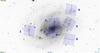 |
Fig. 1 Distribution of the different fields used in this work overlaid on a DSS image of NGC 300. |
3. Photometry and astrometry
3.1. Photometry
The binary fits tables of photometry as defined in Dalcanton et al. (2008) were obtained from the STScI data base. The high image resolution allows stellar point spread function (PSF) photometry in nearby galaxies. This enables studying their different stellar populations in great detail. The photometry was carried out using the package DOLPHOT adapted for the ACS camera (Dolphin 2000).
3.2. Astrometry
Using the ALADIN2 tool to compare the images of each observed NGC 300 field with the respective Dalcanton et al. (2008) catalog, a systematic difference (see Table 1) was found between the World Coordinate System (WCS) indicated in the image headers and those given by the catalog. Then, we compared the positions with the astrometric catalogs UCAC 4 and GSC2.3 and verified that the WCS coordinates were correct. Next we accurately evaluated the difference between the two coordinate systems. To do this, we used the task xy2rd of the IRAF’s3 stsdas package to obtain the WCS coordinates of some (see Table 1) bright and unsaturated stars in the F555W band images of each field. We compared these values with the corresponding ones given by Dalcanton et al. (2008). These corrections were applied to all the objects in this catalog. Finally, we compared each resulting catalog with its corresponding image using ALADIN. The catalogs and images agreed well, although we note that one small relative distortion (~ 0.1′′) still prevailed over some fields.
Corrections applied to the coordinates given by Dalcanton et al. (2008).
3.3. Catalog correlation
The catalogs given by Dalcanton et al. (2008) provide photometric information through three tables for each field, giving in each one the magnitudes of only two bands for each object. We therefore constructed a catalog with the three photometry bands for each field from them. This was performed with the STILTS4 cross-correlation (with logical “OR”) between tables with F555W−F435W bands and those with F814W−F555W bands.
Furthermore, fields 2 and 3 slightly overlap (see Fig. 1), therefore we took a final magnitude for the stars in the overlap region that results from the average between the stars in each field. Using STILTS, we then joined the information and list the two fields as one single field in the table.
4. Searching for young stellar groups
To evaluate the completeness of the data, we built the luminosity function for each table (see Fig. 3). The number of stars per bin begins to decrease below a magnitude F555W= 27. Therefore we considered that the sample is complete for F555W< 26.5.
For better identification throughout the text, we distinguish the following four groups of stars:
-
the blue group: F435W−F555W< 0.25 and F555W–F814W< 0.25;
-
the blue bright group: F555W< 25, F435W−F555W< 0.25 and F555W−F814W< 0.25;
-
the red group: F435W−F555W> 0.6 and F555W–F814W > 0.6;
-
the red bright group: F555W< 25, F435W−F555W> 0.6 and F555W−F814W> 0.6.
In Fig. 2 we show the CMDs of all the stars in the six fields, indicating the previous groups of stars and the location of particular isochrones for solar metallicity (Marigo et al. 2008; Girardi et al. 2010). For the blue bright sample at F555W = 25, the oldest main-sequence turn-off corresponds to 235 Myr, and the lowest stellar mass value for a main-sequence star is ~ 7.4 M⊙.
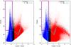 |
Fig. 2 Total CMDs of the six NGC 300 fields with indicative isochrones with solar metallicity (see Sect. 5.4) corresponding to 1 Myr (grey line) and 235 Myr (turquoise line). Inside the rectangle we plot the stars belonging to the blue bright group; red and blue show the red and blue group. |
We used the selected blue bright group to detect young stellar structures, in particular OB associations and young stellar clusters. For this task, we applied different methods that we describe in Sects. 4.1 and 4.2
4.1. Stellar density maps
With the aim of better understanding the distribution of different stellar populations in the galaxy and to have an additional tool to identify young star groups, we used the blue bright group and the red bright group to build spatial density stellar maps for the observed regions. In this process, we constructed for each field a two-dimensional histogram counting the numbers of stars in spatial bin sizes of 8.0 arcsec. Then we applied the drizzle method (Fruchter & Hook 2002) considering a 2.0 arcsec step. The obtained density maps (six) were combined into one image with astrometrical calibration.
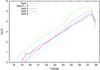 |
Fig. 3 Luminosity functions for the studied fields (fields 2 and 3 are reported as one single field). |
Then, we used the Source Extractor code (SExtractor)5 on the obtained blue stellar density map to identify overdensities that could be identified as young stellar groups. To do this we adopted the default convolution mask of two pixels and assumed a size of four pixels for the background mesh. A larger mesh would imply that the background of the density stellar maps would be too smooth, and therefore some sources might be lost. A detection threshold of 1.5σ above the local background was adopted, and objects with more than four pixels were considered as reliable overdensities. We assumed a value for the deblending contrast parameter δc = 0.001 because this gives the best separation between sources.
The application of this method resulted in the detection of 289 candidates for young groups.
4.2. Path linkage criterion
We also employed the PLC technique (Battinelli 1991) to identify young star groups in NGC 300. This method consists of connecting blue stars that are less distant than a fixed parameter called ds. When it is possible to link more than p stars, we have a candidate OB association or stellar clusters.
We applied this method to the selected blue bright group of stars on each covered field. Then, we had to choose adequate values for the parameters p and ds. The lowest value of the number of stars that a group should have to be considered an association or stellar cluster (p) is a parameter difficult to establish, since a low value results in many spurious detections, while with a high value the smallest groups might be lost. We studied the number of groups identified using PLC with respect to the parameter ds for different values of p (see Fig. 4). Finally, we considered that ten stars is a reasonable value for the parameter p and adopted a value range between 0.5−2.5 arcsec for ds. The advantage of starting the search with a small distance is to detect the smallest subgroups of each large association or stellar complex that otherwise would have been lost in larger structures. After detecting the smallest groups, the star members of these groups were eliminated from the sample and the PLC was run again, but increasing the value of ds. This procedure was repeated until ds reached 2.5 arcsec. Using this method, we detected the individual groups but not the form in which they merge into larger structures. We discuss this point in Sect. 6.2.
Using the PLC technique, we detected 1147 young stellar groups in the six fields.
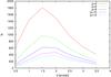 |
Fig. 4 Behavior of the number of groups detected using the PLC technique with respect to the parameter ds for different values of the parameter p. |
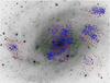 |
Fig. 5 Results obtained using SExtractor (red squares), PLC (blue circles), and the catalog obtained by Pietrzyński et al. (2001; green triangles) overlaid on a DSS image of NGC 300. |
4.3. Results of the search
All the OB associations detected by Pietrzyński et al. (2001) and located in the six ACS fields were found with both techniques used in this work. The obtained detections with the different techniques and the results obtained by Pietrzyński et al. (2001) are shown in Fig. 5, in which we can see from the PLC results that the young stellar groups clearly delineate the spiral structure of the galaxy. The associations identified using the SExtractor code show a more sparse distribution because the group sizes are larger, since the pixels of the density maps are four times larger than the ACS/WFC. This causes several PLC detections to correspond to a single detection of SExtractor. This is a sign of the hierarchical distribution of the blue population in the galaxy, which we address in our discussion (see Sect. 6.2). For this reason and considering that we identified some spurious detections as border effects with SExtractor, we decided to adopt the PLC detections as the final catalog of young stars groups in the galaxy. In Table 2 we show the first ten rows of the catalog, the complete version is available at the CDS.
Young star groups in NGC 300.
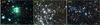 |
Fig. 6 Color images of the associations 2041, 4010, and 5009 located at different galactocentric distances. These groups were detected with the PLC method. |
In Fig. 6 we show three PLC-detected associations at different galactocentric distances. In particular, association 4010 is located in the stellar complex AS002 named by Pietrzyński et al. (2001). As we show in Fig. 7, they detected four subgroups (a, b, c, and d). Using the ASC/HST observations and the PLC method, we detected at least 40 groups in the same region, which are indicated with blue squares in the figure.
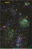 |
Fig. 7 Stellar complex AS002 named by Pietrzyński et al. (2001). The letters a to d designate the four subgroups detected in their work. Our PLC detections are indicated with blue squares. The red rectangle encloses the association 4010, which is shown in Fig. 6. |
5. Analysis
To perform a systematic, homogeneous, and efficient analysis of each identified group, we developed a dedicated numerical code in FORTRAN 95.
5.1. Size and radial density profile
The coordinates of the center and the sizes of the groups were estimated as the mean values and the dispersions of the positions of the blue bright group stars identified for each association.
The density profile was built by distinguishing the different color populations; these are the blue and red group. Then, the stellar density for each color was measured, considering concentric rings with a radial step of 0.4 arcsec. In Fig. 8 we show the radial density profile of association 4010. A clear overdensity of blue stars is evident, while the density of red stars remains equal to zero. This is expected for a young stellar association.
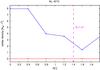 |
Fig. 8 Radial density profile of association 4010. With blue and red we indicate the density of blue and red group stars; the pink dashed line shows the adopted association radius at 1.41′′. |
5.2. Field star decontamination
Our code uses the coordinates of the previously localized groups and performs a statistical decontamination of the field stars based on the magnitudes and color indexes of the stars (see Gallart et al. 2003). The procedure consists of a star-by-star comparison of the quantities F555W, F435W−F555W and F555W−F814W between the stars of the group and the stars of a field region located near the association and covering the same sky area. Then, we subtracted the stars in the group that matched a star in the field region in these quantities. To obtain results as accurate as possible, the code carries out this procedure with five different field regions for each association. The first region is a ring around the association, and the others are selected as follows: (α0 ± Δα, δ0); (α0, δ0 ± Δδ) where Δα = Δδ = 20′′. We discarded the field regions with the largest and smallest number of stars to avoid possible neighboring associations or to fall outside the field of view. The final parameters of an association are an average of the parameters obtained with the three remaining field regions.
From these results we built the photometric diagrams and mass histograms and calculated the fundamental parameters of each group in this way.
5.3. Color–magnitude diagrams
We used the blue and red group to build the color–magnitude diagrams (CMDs) shown in Fig. 9. The evolutionary models of Marigo et al. (2008) with the Girardi et al. (2010) corrections, corresponding to different ages and metallicities, were superposed for comparison. To displace the models and compare them with our data, we adopted a distance modulus of (Vo−MV) = 26.43 (Bresolin et al. 2005), a normal reddening law (R = AV/E(B−V) = 3.1), and a value for E(B−V) = 0.075, where the Galactic foreground reddening toward NGC 300 of 0.025 mag and an additional reddening of E(B−V) = 0.05 mag intrinsic to NGC 300 were considered (Gieren et al. 2004).
The obtained CMDs for most of the identified young star groups revealed a sharp distribution of blue stars. This fact was understood as a consequence of a very low reddening inside the galaxy (Gieren et al. 2004). This situation eliminates possible degeneracy between temperature and extinction for hot stars. Then, as in the following section, we were able to estimate stellar masses from their magnitudes and compare them with fitted theoretical evolutionary models.
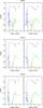 |
Fig. 9 Decontaminated color–magnitude diagrams F555W vs. F435W−F555W and F555W vs. F555W−F814W of the stellar associations 2041, 4010, and 5009 that are located in different places of the galaxy. The blue circles represent the blue group of stars, the red inverted triangle indicate the red group, and the black dots are the stars that are neither blue nor red. The gray line indicates the isochrone corresponding to 107 yr and solar metallicity (Z = 0.019). The green line corresponds to 109 yr and Z = 0.008 (Marigo et al. 2008; Girardi et al. 2010). The arrow indicates the reddening vector. |
5.4. Masses and the present-day mass function
With the purpose of deriving stellar masses, we performed a lineal interpolation in the F555W band in the adopted evolutionary models of 1 Myr (see Sect. 4). To avoid foreground stars in each association, we estimated the stellar masses of the blue-group stars resulting from the statistical decontamination. Given that NGC 300 presents an abundance gradient with Z between 0.004−0.018 (Bresolin et al. 2009; Gazak et al. 2015), we tried to estimate the masses with a range of metallicities between Z = 0.007 and Z = 0.019. Finally, we adopted solar metallicity, since we did not obtain significant differences. The corresponding obtained mass histograms are presented in Fig. 10. Then, using only those bins corresponding to the high-mass range (M>7.4 M⊙, which corresponds to the blue bright group), we performed linear fits to the data. These histograms are representative of the corresponding present-day mass functions (PDMFs). Additionally, in the adopted mass range, the PDMF can be modeled as a power law and expressed in the form log (N/ Δ(log m)) = ΓΔ(log m), where N is the number of stars per logarithmic mass bin log (m). The computed corresponding slope values (Γ) are also indicated in Fig. 10, and the obtained PDMF slopes for each detected association are presented in Table 2.
To estimate the effect of galaxy distance uncertainty and/or possible variable extinction in our procedure, we repeated it for different distance values (26.43 ± 0.09, Bresolin et al. 2005) and using AV values ranging from 0 to 0.53 (Roussel et al. 2005). We obtained that the changes in stellar mass are ΔM/M ~ 25% and changes in the corresponding PDMF slopes are lower than the indicated fitted errors. Therefore, our analysis and conclusions are independent of the above indicated effects.
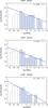 |
Fig. 10 Present-day mass function of the stellar associations 2041, 4010, and 5009 that are located in different places of the galaxy. The line corresponds to a linear fit over the gray bins (M> 7.4 M⊙). |
6. Discussion: Global properties of the young star groups
6.1. Size distribution
From the size distribution of the 1147 young star group detected using the PLC method shown in Fig. 11, we derived that the average radius and the highest value in the distribution are both ~2.5 arcsec. At the considered distance this is approximately equivalent to 25 pc. This value is lower than the one found by Pietrzyński et al. (2001) of ~57 pc. This difference is expected since the HST/ACS images used in this work have higher resolution than the ground-based images. For this reason, they applied the PLC method with a parameter of distance ds much greater than ours (7, 7.5 and 8 arcsec). Bresolin et al. (1998) performed a study of OB association for seven spiral galaxies observed with the HST (NGC 925, NGC 2090, NGC 2541, NGC 3351, NGC 3621, NGC 4548, and M101), finding that the size distribution peaked between radius of 20−40 pc, which is consistent with our value. Pietrzyński et al. (2005) compared these data with several catalogs for OB associations in nearby galaxies in the Local Group (IC 1613, LMC, M 33, NGC 6822, LMC, SMC, and M 31) and some more distant galaxies (UGC 12732, NGC 1058, NGC 7217, NGC 4394, NGC 3507, and NGC 337A). They found a peak in the size distribution between 25−55 pc and an average radius between 20−90 pc for these galaxies. These values agree well with our results.
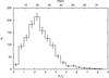 |
Fig. 11 Size distribution of young star groups in NGC 300. |
6.2. Hierarchical structure in NGC 300
It is known that young stars cluster tend to be part of larger groups, such as stellar complexes, which are grouped themselves in larger structures. While we searched for the best-fit distance parameter for the PLC, it became evident that the blue stellar population in NGC 300 presents a hierarchical structure, which starts with the spiral arms and concluds with individual compact clusters, or even with multiple stars. To show this, we traced contours at different density levels on our density stellar maps, created as described in Sect. 4.1. In Fig. 12 we show the different density contours applied to the density maps of the central fields (fields 2 and 3) for the blue bright (left panel) and the red bright group (right panel). The isocontours were created using the tool cont of ALADIN with four different density values (40, 80, 110, and 145 stars per bin of 8 arcsec2); this means different density levels in the density stellar maps. It is clear from Fig. 12 that the blue population follows the spiral arm structure of the galaxy, while the red population is concentrated in the galaxy bulge. The left panel shows several young structures at different density levels. The denser smaller concentrations tend to belong to larger and looser ones, pointing a hierarchical structure in the distribution of blue stars in this galaxy. To easily visualize the ties among structures of different density levels, we built a tree diagram; these types of diagrams are called dendrograms (Gouliermis et al. 2010) and indicate the connection between parent and child structures corresponding to lower and higher density levels, respectively. In Fig. 13 we show the dendrograms of the blue stellar structures identified in the four density levels mentioned above. We added a last level for the most compact structures detected using PLC. The pixels size of the density maps is 2 arcsec, therefore it is not possible to detect the smallest groups that are effectively detected with PLC.
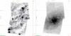 |
Fig. 12 Density maps of central fields for the blue bright group (left panel) and the red bright group (right panel). The overlapping contours correspond to different pixel values, indicating different density levels: black 40, blue 80, red 110, and turquoise 145 stars per bin of 8 arcsec2. |
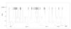 |
Fig. 13 Dendrogram of the young stellar structures detected at different density level. Levels 1–4 correspond to a pixel value in the density maps of 40, 80, 110, and 145, respectively. Level 5 corresponds to the most compact cluster detected using PLC. The blue circles at the bottom indicate the structures detected at the lower density level. Some of them are no longer detected at higher densities. |
6.3. PDMF behavior
Several works have claimed a possible relation between the PDMF shape and the galactocentric distance in galaxies (e.g., Martín-Navarro et al. 2015), since its trend would depend on the local properties within a galaxy. Searching for a possible relation of this kind in NGC 300, we derived the galactocentric distance of each stellar group considering the geometrical parameters of the galaxy given by Puche et al. (1990). These are a position angle γ = 114.3° and an inclination i = 50°. To obtain a more reliable result, we only considered the most relevant stellar groups found in NGC 300, that is, those with the lowest PDMF slope errors (eΓ < 0.5), with massive stars (M > 25 M⊙), and a large number of blue stars (N > 100). Our sample of stellar groups was then 25, and they are plotted in Fig. 14. It seems there is a slight trend for flatter slopes in the outside limit of the galaxy than in the central region (left panel). We found a mean slope of −1.3 ± 0.1 for dGC < 2 kpc and −0.9 ± 0.2 for dGC > 4 kpc. However, within the errors, we are unable to confirm a clear dependence of the Γ slope with the galactocentric distance for NGC 300. We can only indicate their distribution (right panel) and their average and standard deviation (s.d.) values as −1.16 and 0.39, respectively.
7. Conclusions
Using complementary methods for the detection of young stellar groups in NGC 300, we found that the blue population is located in the spiral arms of the galaxy, presenting a hierarchical behavior where denser and smaller structures are enclosed in larger and less dense ones. We were able to delineate the hierarchical structure on several density levels.
Through the PLC technique, 1147 young stellar groups have been detected in six fields of the galaxy NGC 300. The resulting catalog contains the coordinates of the groups, sizes, number of stars, PDMF slope with its error, and galactocentric distance. In Table 2 we present the first ten rows. The completed catalog is available at the CDS. The identification name of each grouping consists of four numbers: the first is the field number, 1, 2, 4, 5, or 6, because fields 2 and 3 were joined into a single field denoted by number 2 (see Sect. 3.3), and the remaining three numbers indicate the number of group in the field.
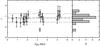 |
Fig. 14 PDMF behavior for the most important groups found in NGC 300 (see text for details). The long dashed line indicates the mean slope value, and the short dashed lines show the envelopes at one standard deviation. |
The mode and the mean of the groups size distribution are both 25 pc. These values agree well with those found in the literature for the Local Group and some more distant galaxies. We did not find a clear dependence of the Γ slope on galactocentric distance for the PDMF of the most important groups, but a slight trend seems to exist that deserves a more detailed analysis. We
can only indicate that the mean value is −1.16 ± 0.39 (s.d.). This slope is slightly flatter than the −1.35 value given by Salpeter (1955) but is compatible within the errors.
IRAF is distributed by NOAO, which is operated by AURA under cooperative agreement with the NSF.
Acknowledgments
We thank the referee for helpful comments and constructive suggestions that helped to improve this paper. M.J.R. and G.B. acknowledge support from CONICET (PIP 112-201101-00301). M.J.R. is a fellow of CONICET. Based on observations made with the NASA/ESA Hubble Space Telescope, and obtained from the Hubble Legacy Archive, which is a collaboration between the Space Telescope Science Institute (STScI/NASA), the Space Telescope European Coordinating Facility (ST-ECF/ESA) and the Canadian Astronomy Data Centre (CADC/NRC/CSA). Some of the data presented in this paper were obtained from the Mikulski Archive for Space Telescopes (MAST). STScI is operated by the Association of Universities for Research in Astronomy, Inc., under NASA contract NAS5-26555. Support for MAST for non-HST data is provided by the NASA Office of Space Science via grant NNX09AF08G and by other grants and contracts. This research has made use of “Aladin sky atlas” developed at CDS, Strasbourg Observatory, France. Finally we would like to thank to Dr. Guido Moyano Layola, the English cabinet of FCAG-UNLP, and the language editor Astrid Peter for English corrections.
References
- Battinelli, P. 1991, A&A, 244, 69 [NASA ADS] [Google Scholar]
- Bresolin, F., Kennicutt, Jr., R. C., Ferrarese, L., et al. 1998, AJ, 116, 119 [NASA ADS] [CrossRef] [Google Scholar]
- Bresolin, F., Pietrzyński, G., Gieren, W., & Kudritzki, R.-P. 2005, ApJ, 634, 1020 [NASA ADS] [CrossRef] [Google Scholar]
- Bresolin, F., Gieren, W., Kudritzki, R.-P., et al. 2009, ApJ, 700, 309 [NASA ADS] [CrossRef] [Google Scholar]
- Dalcanton, J., Williams, B., & ANGST Collaboration 2008, The ACS Nearby Galaxy Survey Treasury: 9 Months of ANGST, eds. H. Jerjen, & B. S. Koribalski, 115 [Google Scholar]
- Dolphin, A. E. 2000, PASP, 112, 1383 [NASA ADS] [CrossRef] [Google Scholar]
- Fruchter, A. S., & Hook, R. N. 2002, PASP, 114, 144 [NASA ADS] [CrossRef] [Google Scholar]
- Gallart, C., Zoccali, M., Bertelli, G., et al. 2003, AJ, 125, 742 [NASA ADS] [CrossRef] [Google Scholar]
- Gazak, J. Z., Kudritzki, R., Evans, C., et al. 2015, ApJ, 805, 182 [NASA ADS] [CrossRef] [Google Scholar]
- Gieren, W., Pietrzyński, G., Walker, A., et al. 2004, AJ, 128, 1167 [NASA ADS] [CrossRef] [Google Scholar]
- Girardi, L., Williams, B. F., Gilbert, K. M., et al. 2010, ApJ, 724, 1030 [NASA ADS] [CrossRef] [Google Scholar]
- Gouliermis, D. A., Schmeja, S., Klessen, R. S., de Blok, W. J. G., & Walter, F. 2010, ApJ, 725, 1717 [NASA ADS] [CrossRef] [Google Scholar]
- Marigo, P., Girardi, L., Bressan, A., et al. 2008, A&A, 482, 883 [NASA ADS] [CrossRef] [EDP Sciences] [Google Scholar]
- Martín-Navarro, I., Barbera, F. L., Vazdekis, A., Falcón-Barroso, J., & Ferreras, I. 2015, MNRAS, 447, 1033 [NASA ADS] [CrossRef] [Google Scholar]
- McConnachie, A. W. 2012, AJ, 144, 4 [NASA ADS] [CrossRef] [Google Scholar]
- Pietrzyński, G., Gieren, W., Fouqué, P., & Pont, F. 2001, A&A, 371, 497 [NASA ADS] [CrossRef] [EDP Sciences] [Google Scholar]
- Pietrzyński, G., Ulaczyk, K., Gieren, W., Bresolin, F., & Kudritzki, R. P. 2005, A&A, 440, 783 [NASA ADS] [CrossRef] [EDP Sciences] [Google Scholar]
- Puche, D., Carignan, C., & Bosma, A. 1990, AJ, 100, 1468 [NASA ADS] [CrossRef] [Google Scholar]
- Roussel, H., Gil de Paz, A., Seibert, M., et al. 2005, ApJ, 632, 227 [NASA ADS] [CrossRef] [Google Scholar]
- Salpeter, E. E. 1955, ApJ, 121, 161 [Google Scholar]
All Tables
All Figures
|
Fig. 1 Distribution of the different fields used in this work overlaid on a DSS image of NGC 300. |
| In the text | |
|
Fig. 2 Total CMDs of the six NGC 300 fields with indicative isochrones with solar metallicity (see Sect. 5.4) corresponding to 1 Myr (grey line) and 235 Myr (turquoise line). Inside the rectangle we plot the stars belonging to the blue bright group; red and blue show the red and blue group. |
| In the text | |
|
Fig. 3 Luminosity functions for the studied fields (fields 2 and 3 are reported as one single field). |
| In the text | |
|
Fig. 4 Behavior of the number of groups detected using the PLC technique with respect to the parameter ds for different values of the parameter p. |
| In the text | |
|
Fig. 5 Results obtained using SExtractor (red squares), PLC (blue circles), and the catalog obtained by Pietrzyński et al. (2001; green triangles) overlaid on a DSS image of NGC 300. |
| In the text | |
|
Fig. 6 Color images of the associations 2041, 4010, and 5009 located at different galactocentric distances. These groups were detected with the PLC method. |
| In the text | |
|
Fig. 7 Stellar complex AS002 named by Pietrzyński et al. (2001). The letters a to d designate the four subgroups detected in their work. Our PLC detections are indicated with blue squares. The red rectangle encloses the association 4010, which is shown in Fig. 6. |
| In the text | |
|
Fig. 8 Radial density profile of association 4010. With blue and red we indicate the density of blue and red group stars; the pink dashed line shows the adopted association radius at 1.41′′. |
| In the text | |
|
Fig. 9 Decontaminated color–magnitude diagrams F555W vs. F435W−F555W and F555W vs. F555W−F814W of the stellar associations 2041, 4010, and 5009 that are located in different places of the galaxy. The blue circles represent the blue group of stars, the red inverted triangle indicate the red group, and the black dots are the stars that are neither blue nor red. The gray line indicates the isochrone corresponding to 107 yr and solar metallicity (Z = 0.019). The green line corresponds to 109 yr and Z = 0.008 (Marigo et al. 2008; Girardi et al. 2010). The arrow indicates the reddening vector. |
| In the text | |
|
Fig. 10 Present-day mass function of the stellar associations 2041, 4010, and 5009 that are located in different places of the galaxy. The line corresponds to a linear fit over the gray bins (M> 7.4 M⊙). |
| In the text | |
|
Fig. 11 Size distribution of young star groups in NGC 300. |
| In the text | |
|
Fig. 12 Density maps of central fields for the blue bright group (left panel) and the red bright group (right panel). The overlapping contours correspond to different pixel values, indicating different density levels: black 40, blue 80, red 110, and turquoise 145 stars per bin of 8 arcsec2. |
| In the text | |
|
Fig. 13 Dendrogram of the young stellar structures detected at different density level. Levels 1–4 correspond to a pixel value in the density maps of 40, 80, 110, and 145, respectively. Level 5 corresponds to the most compact cluster detected using PLC. The blue circles at the bottom indicate the structures detected at the lower density level. Some of them are no longer detected at higher densities. |
| In the text | |
|
Fig. 14 PDMF behavior for the most important groups found in NGC 300 (see text for details). The long dashed line indicates the mean slope value, and the short dashed lines show the envelopes at one standard deviation. |
| In the text | |
Current usage metrics show cumulative count of Article Views (full-text article views including HTML views, PDF and ePub downloads, according to the available data) and Abstracts Views on Vision4Press platform.
Data correspond to usage on the plateform after 2015. The current usage metrics is available 48-96 hours after online publication and is updated daily on week days.
Initial download of the metrics may take a while.