| Issue |
A&A
Volume 593, September 2016
|
|
|---|---|---|
| Article Number | A78 | |
| Number of page(s) | 8 | |
| Section | Extragalactic astronomy | |
| DOI | https://doi.org/10.1051/0004-6361/201628813 | |
| Published online | 26 September 2016 | |
Unresolved versus resolved: testing the validity of young simple stellar population models with VLT/MUSE observations of NGC 3603⋆
1 Millennium Institute of Astrophysics, Casilla 36-D, Santiago, Chile
e-mail: This email address is being protected from spambots. You need JavaScript enabled to view it.
2 Departamento de Astronomía, Universidad de Chile, Casilla 36-D, Santiago, Chile
3 European Southern Observatory, Alonso de Córdova 3107, Vitacura, Casilla 190001, Santiago, Chile
4 Max-Planck-Institut für Extraterrestrische Physik, Giessenbachstraße, 85748 Garching, Germany
Received: 28 April 2016
Accepted: 7 July 2016
Abstract
Context. Stellar populations are the building blocks of galaxies, including the Milky Way. The majority, if not all, extragalactic studies are entangled with the use of stellar population models given the unresolved nature of their observation. Extragalactic systems contain multiple stellar populations with complex star formation histories. However, studies of these systems are mainly based upon the principles of simple stellar populations (SSP). Hence, it is critical to examine the validity of SSP models.
Aims. This work aims to empirically test the validity of SSP models. This is done by comparing SSP models against observations of spatially resolved young stellar population in the determination of its physical properties, that is, age and metallicity.
Methods. Integral field spectroscopy of a young stellar cluster in the Milky Way, NGC 3603, was used to study the properties of the cluster as both a resolved and unresolved stellar population. The unresolved stellar population was analysed using the Hα equivalent width as an age indicator and the ratio of strong emission lines to infer metallicity. In addition, spectral energy distribution (SED) fitting using STARLIGHT was used to infer these properties from the integrated spectrum. Independently, the resolved stellar population was analysed using the colour-magnitude diagram (CMD) to determine age and metallicity. As the SSP model represents the unresolved stellar population, the derived age and metallicity were tested to determine whether they agree with those derived from resolved stars.
Results. The age and metallicity estimate of NGC 3603 derived from integrated spectroscopy are confirmed to be within the range of those derived from the CMD of the resolved stellar population, including other estimates found in the literature. The result from this pilot study supports the reliability of SSP models for studying unresolved young stellar populations.
Key words: galaxies: stellar content / galaxies: star clusters: general / open clusters and associations: individual: NGC 3603 / galaxies: starburst
Based on observations collected at the European Organisation for Astronomical Research in the Southern Hemisphere under ESO programme 60.A-9344.
© ESO, 2016
1. Introduction
Stars together form stellar populations, which are the fundamental building blocks of galaxies in the Universe. A simple stellar population (SSP) is usually defined as a group of stars distributed following an initial mass function (IMF) that was formed from a single cloud of gas with homogeneous chemical composition at the same time in one burst of star formation. As a result, stars within an SSP possess the same age and metallicity. Star clusters have been regarded as nature’s closest approximation to the ideal SSP (cf. Bruzual 2010).
Studies of external galaxies rely heavily on the SSP models. SSP models such as BC03 (Bruzual & Charlot 2003), Starburst99 (Leitherer et al. 1999), and GALEV (Kotulla et al. 2009), among many others, are widely used as probes of unresolved stellar populations in galaxies. SSP models help interpreting the observed spectral energy distribution (SED) into meaningful physical quantities such as age, metallicity, luminosity, stellar content, and star formation rate. Correct determination of such properties is important for the study of galaxies itself as well as for other purposes. For example, in the studies of the hosts and environments of extragalactic transient objects such as supernovae (SNe) and gamma-ray bursts (GRBs), the properties of their stellar progenitors are derived from those of the underlying stellar populations (see e.g. Galbany et al. 2016a,b, 2014; Leloudas et al. 2015, 2011; Krühler et al. 2015; Anderson et al. 2015; Kuncarayakti et al. 2013a,b; Levesque et al. 2010). On that account, correct interpretation of the stellar population associated with the transient is necessary.
While the validity of SSP models is of the utmost importance, there are questions concerning the consistency between different SSP models and whether those are all well tested. Different SSP models are generated using various different methods, thus the stellar population physical properties derived using one SSP model family may not necessarily be consistent with the result from another. The main ingredients of SSP models usually consist of isochrones, a stellar spectral library, and an IMF (see Conroy 2013, for a review). The choice of the isochrones and spectral libraries may be different from one model family to the other, and there can be variations at the more detailed levels such as the stellar evolution calculations for the isochrones and the selection of empirical or theoretical stellar spectra for the library, among others. These differences may eventually affect the constructed SSP models. Figure 1 shows the evolution of the Hα emission line equivalent width (EW) as an age indicator, according to three different SSP model families (GALEV, Starburst99, and BPASS). These SSP models cover very young ages (~Myr) and are thus suitable for the analysis presented here. It is apparent that despite the roughly similar behaviour in evolution, the HαEW values may differ by a factor of two or more at a given age.
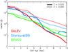 |
Fig. 1 Comparison of the HαEW age indicator of BPASS single-star (Eldridge & Stanway 2009), GALEV (Kotulla et al. 2009), and Starburst99 (Leitherer et al. 1999) SSPs, illustrating the differences between various SSP models. BPASS and GALEV HαEWs were measured directly from the SSP model spectra (see Sect. 3.1 for the measurement method), while in Starburst99 the values are given in tabulated form. All SSP models assume instantaneous star formation and a standard Salpeter IMF. As HαEW also depends on the metallicity of the SSP model, two different metallicities are plotted to illustrate this effect. The solid lines indicate solar metallicity (Z = 0.02) models and the dashed lines models with Z = 0.004. |
To test the validity of SSP models in the analysis of complex extragalactic systems, a two-step procedure is required. First, the SSP models need to be compared to stellar clusters. Second, more complex systems are analysed using combinations of SSP models with non-instantaneous star formation, as one SSP model is considered too simplistic to represent such systems. In the current work, we aim to perform the first step in such a validity test. This first step serves as the basis for the subsequently more intricate step, which eventually will help in assessing whether the SSP-based techniques of extracting stellar population information in extragalactic systems are robust or not.
Attempts to test SSP models against stellar clusters have been undertaken previously, although only for older stellar populations where the massive stars and ionized gas are no longer present (see e.g. Renzini & Fusi Pecci 1988). Beasley et al. (2002) collected integrated spectra of 24 Large Magellanic Cloud star clusters and compared the spectroscopically derived age and metallicity with those from the literature. In general, the age and metallicity derived using Lick/IDS spectral indices show consistency with the literature values, which were mostly derived from the resolved colour-magnitude diagram (CMD) or integrated colour for age and Ca-triplet spectroscopy for metallicity. Other efforts along the same line of study have also been performed by Koleva et al. (2008) and Riffel et al. (2011), who concluded that SSP models quite satisfactorily reproduce the observed parameters, but that there were minor caveats. In the context of studying more complex objects with non-instantaneous star formation history, more recently Ruiz-Lara et al. (2015) presented a comparison of resolved and unresolved stellar populations within a field in the Large Magellanic Cloud in a study of the star formation history in the region.
On the other hand, SSP models corresponding to young stellar populations (~Myr age) are less well established than those for the older population (~Gyr) grids (Conroy 2013). Many SSP models do not include young grids or take into account nebular emissions coming from young stellar populations, while they commonly provide grids for old populations. These young stellar populations are dynamic objects associated with active star-forming regions where the interplay between the ionizing massive stars and the surrounding gas is intense, and energetic events such as core-collapse SNe and long-GRBs occur (see e.g. Portegies Zwart et al. 2010). Even in a galaxy preeminently consisting of old stellar populations, the young populations may dominate the emissions in the ultraviolet/optical regime, thus affecting significantly the observed integrated properties (Meurer et al. 1995; Anders & Fritze-v. Alvensleben 2003).
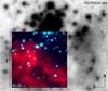 |
Fig. 2 Pseudo-RGB colour image of the MUSE field of view (FoV) of NGC 3603 generated from the datacube, superposed on a POSS2-red image from the Digitized Sky Survey (DSS). North is up and east is to the left. Each side of MUSE FoV is approximately 1 arcmin (corresponding to 2 pc at the distance of 7 kpc). The core of the cluster lies just outside the FoV in the north-north-west direction and was intentionally missed in the observations to avoid severe crowding. Red corresponds to Hα and blue and green correspond to the continuum at 4700 and 5500 Å, respectively. The stars whose spectra are shown in Fig. 3 are indicated with their identification numbers, based on the WEBDA catalogue. |
In this paper we report our pilot study of examining the reliability of young SSP models, for which we used VLT/MUSE integral field spectroscopy (IFS) of a well-studied young stellar population, NGC 3603. It has been suggested that the cluster is as young as a few Myr (e.g. Melnick et al. 1989; Sagar et al. 2001) and was formed in an instantaneous burst of star formation (Kudryavtseva et al. 2012; Fukui et al. 2014). It therefore represents a good approximation for a young SSP. As young stellar populations are still associated with ionized gas, IFS offers the most efficient way to obtain the integrated spectrum of the cluster, including the ionized gas, in addition to the individual spectra of the member stars. With this technique, it is possible to obtain simultaneously the integrated and resolved information of a stellar population from a single dataset. This would have taken enormous time to conduct with conventional slit or fiber spectroscopy, and to our knowledge, this is the first such effort of testing young (~Myr) SSP models.
The paper is organized as follows. Following the introduction, the observations and data reduction are described in Sect. 2, then the analysis of the integrated spectrum for age and metallicity estimates is presented in Sect. 3. In Sect. 4 we analyse the properties of the resolved stars and compare them to the unresolved stellar population from the integrated light. Section 5 provides a final summary.
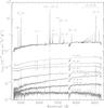 |
Fig. 3 Observed integrated spectrum of NGC 3603 within the whole MUSE FoV (top; solid black line), plotted alongside a montage of spectra from several individual stars in the field (solid grey lines). The individual stars are identified with their respective identification numbers (see Fig. 2). The integrated spectrum is the sum of all the spaxels in the FoV and thus includes all the individual stellar spectra and the associated nebulosity. The strongest emission lines in the integrated spectrum are indicated. Spectra are wavelength and flux calibrated. |
2. Observations and data reduction
The observations were conducted using the Multi-Unit Spectroscopic Explorer (MUSE) integral field spectrograph (Bacon et al. 2014) of the Very Large Telescope (VLT) at the Cerro Paranal Observatory, Chile. As part of the MUSE Science Verification run, NGC 3603 was observed on 2014 June 29 (Programme 60.A-9344, PI: Kuncarayakti1). MUSE was used in the Wide Field Mode, giving a field of view (FoV) of 1 arcmin2 sampled by 0.2′′× 0.2′′ spaxels across 4650−9300 Å. The mean spectral resolution is around 3000, with dispersion of 1.25 Å/pixel. The observations were made in non-photometric conditions under ~0.8′′ seeing. The raw data were reduced using the MUSE data reduction pipeline integrated within the Reflex environment (Freudling et al. 2013), which includes procedures of bias subtraction, flatfielding, subtraction of sky from blank sky pointings, wavelength and flux calibrations, spectral extraction and datacube reconstruction. The resulting datacube from a single 300 s integration was used in this work. Figure 2 shows a pseudo-RGB image of the whole MUSE FoV of NGC 3603. The image quality had a full width at half maximum (FWHM) ≈ 0.8′′ as measured in the collapsed datacube, consistent with the seeing monitor, demonstrating the excellent performance of MUSE.
The datacube was subsequently analysed using the QFitsView2 visualisation software (Ott 2012) and IRAF3. We extracted the spectrum over the full MUSE FoV, integrating at the same time the spectra of individual stars and the interstellar diffuse light. Figure 3 shows the integrated spectrum of NGC 3603, exhibiting a multitude of strong emission lines emitted by the ionized gas superposed on a continuum originating from the stellar component. A montage of several individual stellar spectra is also shown in the figure. The individual stellar spectra were extracted using an aperture of comparable size to the point spread function FWHM, that is, 4 spaxels (0.8′′) radius. These integrated and individual spectra were then used in the subsequent analyses. VRI magnitudes of the individual stars were also calculated by applying synthetic photometry to the individual stellar spectra. These were then cross-matched and compared with the entries at the WEBDA4 online stellar clusters database. As our observations were made under non-photometric conditions, there were zero-point offsets between our synthetic VRI magnitudes with the photometry available at WEBDA, which were taken from the work of Sagar et al. (2001). We calculated the mean offsets for each filter and applied them to the synthetic magnitudes of each star.
3. Analysis of the integrated spectrum
The integrated spectrum of NGC 3603 is considered analogous to that of an unresolved stellar population that has been observed spectroscopically. The spectrum contains the continuum emission contributed by the individual stars and the nebular component emitted by the surrounding ionized gas.
The age and metallicity of the cluster were derived using two independent methods that both use SSP models. The first method uses the emission lines; it compares the equivalent width of the Hα emission line with SSP models to determine the age at a fixed metallicity, the latter derived through the strong-line method. The second method fits the continuum of the integrated spectrum with the SED of SSP models to simultaneously determine the age and metallicity.
3.1. Emission line analysis
The equivalent width of the Hα emission line (HαEW) is used to derive the stellar population age. As it measures the flux ratio between the line emission from the ionized gas and the continuum light emitted by the stellar component, it is proportional to the number ratio of massive, ionizing OB stars compared to the lower mass, non-ionizing stars. Thus in an SSP it is expected that the HαEW decreases over time as the short-lived massive stars die first, even though all the SSP stars are of the same age (see Fig. 1). The use of HαEW as a good age indicator for young stellar populations has been demonstrated for instance by Reines et al. (2010), Leloudas et al. (2011), and Kuncarayakti et al. (2013a,b).
From the integrated MUSE spectrum of NGC 3603 we measured the HαEW and the gas-phase metallicity in terms of oxygen abundance. The abundance was derived first as the evolution models of HαEW depend on the assumed metallicity (see Fig. 1). We used the strong-line method with the N2 (Storchi-Bergmann et al. 1994) and O3N2 (Alloin et al. 1979) indices calibrated according to Marino et al. (2013). Using the task splot within the onedspec package in IRAF, the emission line fluxes were measured to determine the metallicity. The derived metallicity for NGC 3603 from the N2 index is 12 + log(O/H) = 8.09 dex, while it is 12 + log(O/H) = 8.07 dex from the O3N2 index. The averaged metallicity therefore corresponds to Z = 0.0034 assuming a solar oxygen abundance of 12 + log(O/H)⊙ = 8.69 dex or Z⊙ = 0.014 (Asplund et al. 2009). For the subsequent analysis, the SSP models with the metallicity value nearest to Z = 0.004 were used.
Again using splot , the HαEW of NGC 3603 was measured to be 378±0.3 Å. The same measurement method was also employed for GALEV and BPASS SSP spectra, resulting in the HαEW evolution shown in Fig. 1. This observed HαEW of NGC 3603 was then compared to the Starburst99 SSP models with Z = 0.004 and a standard Salpeter IMF (α = 2.35, Mup = 100M⊙), yielding an age of 5.05 Myr. As a cross check we derived a value of HαEW = 355 Å with ROBOSPECT, an automatic spectral line equivalent width measurement software (Waters & Hollek 2013). This corresponds to a similar age of 5.09 Myr with the same Starburst99 SSP.
Using the HαEW value from the splot measurement, age estimates were also derived using GALEV and BPASS SSP models. With models of the same Z = 0.004 metallicity, the resulting age estimates were 5.74 and 3.94 Myr for GALEV and BPASS, respectively. Although the results of the three SSP model families are consistent at the value of around 4−6 Myr, in line with Fig. 1, this illustrates the different outcomes in estimating stellar population age when using different sets of SSP models.
3.2. SED fitting
We furthermore analysed the integrated spectrum of NGC 3603 using the STARLIGHT code (Cid Fernandes et al. 2005) to estimate the age and metallicity. STARLIGHT fits the observed SED with a library of SSP model spectra with different ages and metallicities and returns the best combination of SSP spectra that matches the object SED. The fitting was made to the continuum and absorption lines, but the emission lines were masked out. The fitting process is similar to the one described in Galbany et al. (2014), only with a different wavelength range because MUSE does not cover the blue part of the optical spectrum. We used the spectral range from 4650 Å for the fit and experimented with different red wavelength cutoffs. Fitting the whole MUSE spectral range up to 9300 Å generally increases contamination from old stellar populations, and the fitting was found to be optimal (i.e. dominated by young population) when limited to around 7000 Å.
The spectral library used by our STARLIGHT fit consists of 66 SSP spectra, each with different ages and metallicity. These were modified from Bruzual & Charlot (2003) SSP models (see Bruzual 2007) using the MILES spectral library (Sánchez-Blázquez et al. 2006), a Chabrier IMF, the Padova 1994 evolutionary tracks, and TP-AGB star recipes by Marigo & Girardi (2007) and Marigo et al. (2008).
From the SED fitting, STARLIGHT found that the integrated spectrum of NGC 3603 is best matched by an SSP with a log age of 6.61 (≈4.1 Myr) and metallicity Z = 0.008, additionally with negligible contribution from older SSPs of log age ≈ 8 and 10. This 4 Myr estimate agrees well with the 4−6 Myr result from the HαEW method. For a comparison, we also tried to use a different SSP model for the fitting (González Delgado et al. 2005). The best fit contains a stellar population with an age of 3.0 Myr, although with significantly higher metallicity of Z = 0.03 and heavier contamination from the old populations in which they became the dominant component. Therefore, the result using Bruzual (2007) SSP models was preferred. Figure 4 shows the STARLIGHT fits compared to the observed integrated spectrum of NGC 3603. It is interesting to note that although the Bruzual (2007) and González Delgado et al. (2005) SSP models produce very similar fits, the age and metallicity solutions are markedly different.
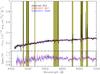 |
Fig. 4 Result of the STARLIGHT fit using the SSP models from Bruzual (2007, red) and González Delgado et al. (2005, blue) compared to the integrated spectrum of NGC 3603 (black). Masked regions are shaded in dark yellow. Fit residuals are shown in the bottom panel. The horizontal dashed line indicates the ratio of unity between the observed spectrum and model fit. |
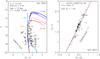 |
Fig. 5 Left: Colour–magnitude diagram of NGC 3603, constructed using synthetic photometry (open black circles). Filled grey circles represent the WEBDA catalogue magnitudes (Sagar et al. 2001), shown for comparison. Isochrones of Z = 0.004, log t = 6.0 (1 Myr, cyan) and 7.0 (10 Myr, blue) are plotted with solid lines, those of the same ages at Z = 0.008 with dashed lines. Non-fitting isochrones of 20 Myr are also plotted (red). The position of the main-sequence turn-off point (MSTO) is indicated with a yellow circle. Right: two-colour diagram of NGC 3603, also constructed using synthetic photometry (open black circles). The solid black line indicates a linear regression, the dashed red line the normal interstellar extinction law. Following Sagar et al. (2001), colour excess ratios of E(V−R) /E(B−V) = 0.65 (Alcalá & Arellano Ferro 1988) and E(V−I) /E(B−V) = 1.25 (Dean et al. 1978) are used for the normal extinction law. The directions of the normal reddening vectors are shown with arrows in both diagrams. |
4. Comparison with the resolved stellar population
With the age and metallicity of NGC 3603 derived from the integrated spectrum, we now consider the estimates determined from the individual stars that are part of NGC 3603. As resolved stars are considered to be the canonical form of stellar populations, such a comparison enables assessing the reliability of the SSP models. If the SSP models are correct, then the properties derived from integrated spectrum should match those derived from the resolved stellar population.
In most cases in the literature, the age of NGC 3603 was derived using the CMD, a common method to analyse stellar clusters in which the photometry of the individual stars is compared to theoretical isochrones to derive simultaneously the cluster age, metallicity, distance, and reddening. Previously, it has generally been found that NGC 3603 contains a very young stellar population with an age of a few Myr and a metallicity of about solar or lower, although there is no consensus as to the exact age, and the metallicity has not been discussed so far.
Melnick et al. (1989) presented UBV CCD photometry of the cluster and inferred an age between 2 and 3 Myr based on the CMD, with a spread of 2 Myr. They supplemented their analysis with a metallicity estimate for which they used slit spectroscopy of the associated nebula. This yielded 12 + log(O/H) = 8.39. Subsequently, using UBVRI photometry, Pandey et al. (2000) concluded a mean cluster age of ≲ 1 Myr with an age spread of a few Myr within the cluster, and Sagar et al. (2001) found an age of 3±2 Myr. Sung & Bessell (2004) resolved the inner core and studied the stellar content of the cluster by using Hubble Space Telescope (HST) Wide Field and Planetary Camera 2 (WFPC2) observations. They derived an age of 1±1 Myr for the inner part of the cluster and ≲ 5 Myr for the outer parts. Before the HST, well-resolved observations of the inner part of the cluster were not available. Later, Melena et al. (2008) used HST Advanced Camera for Surveys (ACS) images to corroborate this result, finding that the most massive stars (some reach ≳ 120M⊙) are coeval within 1−2 Myr, but there could be an age spread of up to 4 Myr in the cluster. Based on ground-based high spatial resolution adaptive optics observations in the near-infrared, Harayama et al. (2008) derived an age of ≲ 2.5 Myr for the cluster.
Age and metallicity estimates obtained in this study, compared to previous works.
Some estimates using the lower part of the CMD that contains the pre-main sequence (PMS) stars may suggest different ages. Beccari et al. (2010) derived an age spread between 1−20 Myr assuming solar metallicity, Z⊙ = 0.019. In contrast, Kudryavtseva et al. (2012) provided an age estimate of 2±0.1 Myr with an assumed solar metallicity of Z⊙ = 0.015, which is more consistent with the estimates from the upper CMD. Harayama et al. (2008) also estimated an age of 0.5−1.0 Myr for the PMS stars in NGC 3603. While this aspect of PMS stars is interesting in itself, it is beyond the scope of this paper, and in the current context it is more meaningful to compare the SSP results with those from the upper CMD, as the lower CMD contributes only a negligible amount to the integrated output light of the stellar population.
We demonstrate that our integral field spectroscopy is able to reproduce the photometry and the cluster CMD, on which a procedure of isochrone fitting was performed to estimate the cluster age. The isochrones used were taken from the PARSEC database (Bressan et al. 2012). Figure 5 shows the CMD and two-colour diagram that are commonly used in resolved stellar population studies, generated using the synthetic magnitudes calculated from the individual star spectra. The diagrams contain 68 individual stars within the FoV. The CMD of NGC 3603 shows a well-defined main sequence, with a contamination of foreground stars suffering less reddening than the cluster stars, on the blue side of the main sequence at (V−I) < 1.4.
In the CMD (Fig. 5), the cluster main-sequence turn-off (MSTO) point is indicated. It is the position where, starting with the most massive stars within the cluster, stars begin to depart from the zero-age main sequence (ZAMS; here represented by the 1 Myr isochrone) and moving towards the (super)giant branch. Therefore, the MSTO essentially signifies the position of the bluest and most massive star still on the main sequence. In an SSP with zero extinction, the distribution of the position of the stars would closely follow the isochrone shape. In reality, in most clusters the observed main sequence is broadened as stars are spread redwards of the isochrone along the reddening vector. NGC 3603 suffers from this effect of differential reddening (Sagar et al. 2001; Melena et al. 2008) and displays such a broadened main sequence. Thus, the position of a star in the CMD does not necessarily reflect its actual position on the isochrone. Its actual, dereddened, position lies on the isochrone in the direction of the reverse of the reddening vector. The star’s position cannot be bluer than the isochrone. In NGC 3603, the stars above the MSTO could belong to the 10 Myr isochrone or younger, but not to the older ones (e.g. 20 Myr) as the isochrone would be too red compared to those stars. Therefore, it is unlikely that the cluster is older than 10 Myr.
Thus, in the CMD the photometry can be well fit with isochrones of ages younger than 10 Myr for both Z = 0.004 and Z = 0.008, while fixing the values of distance and reddening as given in Sagar et al. (2001), that is, d = 7.2 kpc, E(B−V) = 1.44. The adopted values of distance and reddening differ by only about 10% from those in the other references (e.g. d = 6.3 kpc, E(B−V) = 1.48, Pandey et al. 2000; d = 7.6 kpc, E(B−V) = 1.39, Melena et al. 2008). It was also noted by Melena et al. (2008) that there is very good agreement on the derived apparent distance modulus of NGC 3603 in the literature, with the uncertainty on the physical distance stemming mainly from the extinction uncertainty.
The two-colour diagram also shows that the interstellar extinction law towards the direction of NGC 3603 is quite normal, in agreement with the result of Sagar et al. (2001). Varying the metallicity of the isochrone does not affect the isochrone fitting as the isochrone shape is only weakly sensitive to metallicity variation. However, isochrones are very age-sensitive, and in this case, the age solution is limited up to 10 Myr, as beyond this age the cluster turn-off point would move too far downward.
This upper limit of 10 Myr does not contradict our spectroscopic age estimate of 4−6 Myr. Furthermore, the photometric ages found in the literature agree reasonably well with the spectroscopic age estimate. It has been reported that the age of the stars in the outer part of the cluster reaches up to 4−5 Myr (Melnick et al. 1989; Pandey et al. 2000; Sagar et al. 2001; Sung & Bessell 2004; Melena et al. 2008). Our analysis here corresponds more closely to this outer region. Table 1 presents our estimates of age and metallicity compared to a number of references. These indicate that the age estimates derived from resolved and unresolved stellar populations are broadly consistent. We note that some caveats may apply to the CMD and isochrone fitting, such as differential reddening, binarity, sequential star formation, field star contamination and selections of stars included in analysis, as well as different isochrone prescriptions. On the other hand, the SSP models used in the spectroscopic analysis are also subject to different prescriptions used to generate them, as demonstrated in Fig. 1. We note that our FoV does not contain the whole extent of the NGC 3603 cluster and the associated nebula5 (see Fig. 2), which may affect the derived properties. Finally, owing to the low number of stars in our CMD, the result is not very constraining compared to the other CMD results in the literature, which converge at around 1−5 Myr.
We point out that the direct comparison between photometry and spectroscopy in the context of metallicity determination was not conclusive because of the nature of the isochrones. The methods using isochrone or SED fitting are not very sensitive to metallicity variations, therefore they are generally considered inferior compared to the strong-line method in determining metallicity. However, we confirm for NGC 3603 that the metallicity values obtained from the integrated spectrum can be accommodated by isochrone fitting. In Table 1 the reference metallicities are assumed or derived spectroscopically.
5. Summary
We have obtained integral field spectroscopy of NGC 3603 using VLT/MUSE, from which an analysis to determine age and metallicity was performed with the aim of testing the validity of SSP models. The integrated spectrum of NGC 3603 was analysed with the strong-line method, together with SSP model comparisons to both the HαEW and the overall SED. The resulting age and metallicity were then compared to those derived from an independent method utilizing the color–magnitude diagram of resolved stellar population from this very dataset, and also to other age and metallicity estimates obtained from the literature.
From the integrated spectrum the age of NGC 3603 was derived to be about 4−6 Myr with a metallicity between Z = 0.004 and Z = 0.008. The uncertainty in the age estimate originates from the different results when comparing the observed HαEW to the different SSP models (BPASS/GALEV/Starburst99). In the case of SED fitting, using different SSP models similarly alters the age estimate, although this also results in strong variations in metallicity and in the fraction of contamination from older populations. Overall, this illustrates the notion that using different SSP models may yield different results in the interpretation of stellar population properties.
The 4−6 Myr age estimate from the integrated spectrum agrees reasonably well with the estimates from photometry (~1−5 Myr) and suggests that the two independent methods are consistent. This pilot study provides a promising start towards a more systematic and comprehensive investigation in the effort of testing SSP models for young stellar populations. In this context, IFS offers a unique way of performing such an investigation because of the extended nature of the ionized gas component in young stellar populations. MUSE as the foremost IFS instrument currently available offers the exciting capability of exploring the stellar content and nebular component of young star clusters simultaneously. For systems located close enough so as to have a good spatial resolution, MUSE allows both resolved stellar population and integrated population analyses. Wide-field IFS observations of young stellar clusters with a significantly larger sample are desired to further advance this study, opening the possibility of a new field of analysis. We encourage the community to undertake efforts such as the one presented here in comparing resolved and unresolved stellar populations. This would help in refining SSP analysis techniques, which is ultimately vital for our understanding of extragalactic systems.
Shared observation programme with PIs Vink and González-Fernández as in the MUSE Science Verification run similar proposals were combined together for efficiency.
IRAF is distributed by the National Optical Astronomy Observatory, which is operated by the Association of Universities for Research in Astronomy (AURA) under cooperative agreement with the National Science Foundation.
A mosaic observation was requested but not obtained due to limitations in the science verification run of the instrument.
Acknowledgments
The authors thank the anonymous referee, whose valuable comments and suggestions helped improve the paper. We also wish to thank Patricia Sánchez-Blázquez, Mamoru Doi, and Nobuo Arimoto for reading and providing useful comments for the manuscript. Support for H.K., L.G., and M.H. is provided by the Ministry of Economy, Development, and Tourism’s Millennium Science Initiative through grant IC120009, awarded to The Millennium Institute of Astrophysics, MAS. H.K. and L.G. acknowledge support by CONICYT through FONDECYT grants 3140563 and 3140566, respectively. T.K. acknowledges support through the Sofja Kovalevskaja Award to P. Schady from the Alexander von Humboldt Foundation of Germany. We acknowledge great help provided by the MUSE Science Verification Team. Based on observations collected at the European Organisation for Astronomical Research in the Southern Hemisphere under ESO programme 60.A-9344. This research has made use of the WEBDA database, operated at the Department of Theoretical Physics and Astrophysics of the Masaryk University.
References
- Alcalá, J. M., & Arellano Ferro, A. 1988, Rev. Mexicana Astron. Astrofis., 16, 81 [NASA ADS] [Google Scholar]
- Alloin, D., Collin-Souffrin, S., Joly, M., & Vigroux, L. 1979, A&A, 78, 200 [Google Scholar]
- Anders, P., & Fritze-v.Alvensleben, U. 2003, A&A, 401, 1063 [NASA ADS] [CrossRef] [EDP Sciences] [Google Scholar]
- Anderson, J. P., James, P. A., Habergham, S. M., Galbany, L., & Kuncarayakti, H. 2015, PASA, 32, e019 [NASA ADS] [CrossRef] [Google Scholar]
- Asplund, M., Grevesse, N., Sauval, A. J., & Scott, P. 2009, ARA&A, 47, 481 [NASA ADS] [CrossRef] [Google Scholar]
- Bacon, R., Vernet, J., Borisova, E., et al. 2014, The Messenger, 157, 13 [NASA ADS] [Google Scholar]
- Beasley, M. A., Hoyle, F., & Sharples, R. M. 2002, MNRAS, 336, 168 [NASA ADS] [CrossRef] [Google Scholar]
- Beccari, G., Spezzi, L., De Marchi, G., et al. 2010, ApJ, 720, 1108 [NASA ADS] [CrossRef] [Google Scholar]
- Bressan, A., Marigo, P., Girardi, L., et al. 2012, MNRAS, 427, 127 [NASA ADS] [CrossRef] [Google Scholar]
- Bruzual, G. 2007, in From Stars to Galaxies: Building the Pieces to Build Up the Universe, ASP Conf. Ser., 374, 303 [NASA ADS] [Google Scholar]
- Bruzual, A. G. 2010, Phil. Trans. R. Soc. Lond. Ser. A, 368, 783 [NASA ADS] [CrossRef] [Google Scholar]
- Bruzual, G., & Charlot, S. 2003, MNRAS, 344, 1000 [NASA ADS] [CrossRef] [Google Scholar]
- Cid Fernandes, R., Mateus, A., Sodré, L., Stasińska, G., & Gomes, J. M. 2005, MNRAS, 358, 363 [NASA ADS] [CrossRef] [Google Scholar]
- Conroy, C. 2013, ARA&A, 51, 393 [NASA ADS] [CrossRef] [Google Scholar]
- Dean, J. F., Warren, P. R., & Cousins, A. W. J. 1978, MNRAS, 183, 569 [NASA ADS] [CrossRef] [Google Scholar]
- Eldridge, J. J., & Stanway, E. R. 2009, MNRAS, 400, 1019 [NASA ADS] [CrossRef] [Google Scholar]
- Freudling, W., Romaniello, M., Bramich, D. M., et al. 2013, A&A, 559, A96 [NASA ADS] [CrossRef] [EDP Sciences] [Google Scholar]
- Fukui, Y., Ohama, A., Hanaoka, N., et al. 2014, ApJ, 780, 36 [NASA ADS] [CrossRef] [Google Scholar]
- Galbany, L., Stanishev, V., Mourão, A. M., et al. 2014, A&A, 572, A38 [NASA ADS] [CrossRef] [EDP Sciences] [Google Scholar]
- Galbany, L., Anderson, J. P., Rosales-Ortega, F. F., et al. 2016a, MNRAS, 455, 4087 [NASA ADS] [CrossRef] [Google Scholar]
- Galbany, L., Stanishev, V., Mourão, A. M., et al. 2016b, A&A, 591, A48 [NASA ADS] [CrossRef] [EDP Sciences] [Google Scholar]
- González Delgado, R. M., Cerviño, M., Martins, L. P., Leitherer, C., & Hauschildt, P. H. 2005, MNRAS, 357, 945 [NASA ADS] [CrossRef] [Google Scholar]
- Harayama, Y., Eisenhauer, F., & Martins, F. 2008, ApJ, 675, 1319 [NASA ADS] [CrossRef] [Google Scholar]
- Koleva, M., Prugniel, P., Ocvirk, P., Le Borgne, D., & Soubiran, C. 2008, MNRAS, 385, 1998 [NASA ADS] [CrossRef] [Google Scholar]
- Kotulla, R., Fritze, U., Weilbacher, P., & Anders, P. 2009, MNRAS, 396, 462 [NASA ADS] [CrossRef] [Google Scholar]
- Krühler, T., Malesani, D., Fynbo, J. P. U., et al. 2015, A&A, 581, A125 [NASA ADS] [CrossRef] [EDP Sciences] [Google Scholar]
- Kudryavtseva, N., Brandner, W., Gennaro, M., et al. 2012, ApJ, 750, L44 [NASA ADS] [CrossRef] [Google Scholar]
- Kuncarayakti, H., Doi, M., Aldering, G., et al. 2013a, AJ, 146, 30 [NASA ADS] [CrossRef] [Google Scholar]
- Kuncarayakti, H., Doi, M., Aldering, G., et al. 2013b, AJ, 146, 31 [NASA ADS] [CrossRef] [Google Scholar]
- Leitherer, C., Schaerer, D., Goldader, J. D., et al. 1999, ApJS, 123, 3 [NASA ADS] [CrossRef] [Google Scholar]
- Leloudas, G., Gallazzi, A., Sollerman, J., et al. 2011, A&A, 530, A95 [NASA ADS] [CrossRef] [EDP Sciences] [Google Scholar]
- Leloudas, G., Schulze, S., Krühler, T., et al. 2015, MNRAS, 449, 917 [NASA ADS] [CrossRef] [Google Scholar]
- Levesque, E. M., Soderberg, A. M., Kewley, L. J., & Berger, E. 2010, ApJ, 725, 1337 [NASA ADS] [CrossRef] [Google Scholar]
- Marigo, P., & Girardi, L. 2007, A&A, 469, 239 [NASA ADS] [CrossRef] [EDP Sciences] [Google Scholar]
- Marigo, P., Girardi, L., Bressan, A., et al. 2008, A&A, 482, 883 [NASA ADS] [CrossRef] [EDP Sciences] [Google Scholar]
- Marino, R. A., Rosales-Ortega, F. F., Sánchez, S. F., et al. 2013, A&A, 559, A114 [NASA ADS] [CrossRef] [EDP Sciences] [Google Scholar]
- Melena, N. W., Massey, P., Morrell, N. I., & Zangari, A. M. 2008, AJ, 135, 878 [NASA ADS] [CrossRef] [Google Scholar]
- Melnick, J., Tapia, M., & Terlevich, R. 1989, A&A, 213, 89 [NASA ADS] [Google Scholar]
- Meurer, G. R., Heckman, T. M., Leitherer, C., et al. 1995, AJ, 110, 2665 [NASA ADS] [CrossRef] [Google Scholar]
- Ott, T. 2012, Astrophysics Source Code Library [record ascl:1210.019] [Google Scholar]
- Pandey, A. K., Ogura, K., & Sekiguchi, K. 2000, PASJ, 52, 847 [NASA ADS] [CrossRef] [Google Scholar]
- Portegies Zwart, S. F., McMillan, S. L. W., & Gieles, M. 2010, ARA&A, 48, 431 [NASA ADS] [CrossRef] [Google Scholar]
- Reines, A. E., Nidever, D. L., Whelan, D. G., & Johnson, K. E. 2010, ApJ, 708, 26 [NASA ADS] [CrossRef] [Google Scholar]
- Renzini, A., & Fusi Pecci, F. 1988, ARA&A, 26, 199 [NASA ADS] [CrossRef] [Google Scholar]
- Riffel, R., Ruschel-Dutra, D., Pastoriza, M. G., et al. 2011, MNRAS, 410, 2714 [NASA ADS] [CrossRef] [Google Scholar]
- Ruiz-Lara, T., Pérez, I., Gallart, C., et al. 2015, A&A, 583, A60 [NASA ADS] [CrossRef] [EDP Sciences] [Google Scholar]
- Sagar, R., Munari, U., & de Boer, K. S. 2001, MNRAS, 327, 23 [NASA ADS] [CrossRef] [Google Scholar]
- Sánchez-Blázquez, P., Peletier, R. F., Jiménez-Vicente, J., et al. 2006, MNRAS, 371, 703 [NASA ADS] [CrossRef] [Google Scholar]
- Storchi-Bergmann, T., Calzetti, D., & Kinney, A. L. 1994, ApJ, 429, 572 [NASA ADS] [CrossRef] [Google Scholar]
- Sung, H., & Bessell, M. S. 2004, AJ, 127, 1014 [NASA ADS] [CrossRef] [Google Scholar]
- Waters, C. Z., & Hollek, J. K. 2013, PASP, 125, 1164 [NASA ADS] [CrossRef] [Google Scholar]
All Tables
Age and metallicity estimates obtained in this study, compared to previous works.
All Figures
|
Fig. 1 Comparison of the HαEW age indicator of BPASS single-star (Eldridge & Stanway 2009), GALEV (Kotulla et al. 2009), and Starburst99 (Leitherer et al. 1999) SSPs, illustrating the differences between various SSP models. BPASS and GALEV HαEWs were measured directly from the SSP model spectra (see Sect. 3.1 for the measurement method), while in Starburst99 the values are given in tabulated form. All SSP models assume instantaneous star formation and a standard Salpeter IMF. As HαEW also depends on the metallicity of the SSP model, two different metallicities are plotted to illustrate this effect. The solid lines indicate solar metallicity (Z = 0.02) models and the dashed lines models with Z = 0.004. |
| In the text | |
|
Fig. 2 Pseudo-RGB colour image of the MUSE field of view (FoV) of NGC 3603 generated from the datacube, superposed on a POSS2-red image from the Digitized Sky Survey (DSS). North is up and east is to the left. Each side of MUSE FoV is approximately 1 arcmin (corresponding to 2 pc at the distance of 7 kpc). The core of the cluster lies just outside the FoV in the north-north-west direction and was intentionally missed in the observations to avoid severe crowding. Red corresponds to Hα and blue and green correspond to the continuum at 4700 and 5500 Å, respectively. The stars whose spectra are shown in Fig. 3 are indicated with their identification numbers, based on the WEBDA catalogue. |
| In the text | |
|
Fig. 3 Observed integrated spectrum of NGC 3603 within the whole MUSE FoV (top; solid black line), plotted alongside a montage of spectra from several individual stars in the field (solid grey lines). The individual stars are identified with their respective identification numbers (see Fig. 2). The integrated spectrum is the sum of all the spaxels in the FoV and thus includes all the individual stellar spectra and the associated nebulosity. The strongest emission lines in the integrated spectrum are indicated. Spectra are wavelength and flux calibrated. |
| In the text | |
|
Fig. 4 Result of the STARLIGHT fit using the SSP models from Bruzual (2007, red) and González Delgado et al. (2005, blue) compared to the integrated spectrum of NGC 3603 (black). Masked regions are shaded in dark yellow. Fit residuals are shown in the bottom panel. The horizontal dashed line indicates the ratio of unity between the observed spectrum and model fit. |
| In the text | |
|
Fig. 5 Left: Colour–magnitude diagram of NGC 3603, constructed using synthetic photometry (open black circles). Filled grey circles represent the WEBDA catalogue magnitudes (Sagar et al. 2001), shown for comparison. Isochrones of Z = 0.004, log t = 6.0 (1 Myr, cyan) and 7.0 (10 Myr, blue) are plotted with solid lines, those of the same ages at Z = 0.008 with dashed lines. Non-fitting isochrones of 20 Myr are also plotted (red). The position of the main-sequence turn-off point (MSTO) is indicated with a yellow circle. Right: two-colour diagram of NGC 3603, also constructed using synthetic photometry (open black circles). The solid black line indicates a linear regression, the dashed red line the normal interstellar extinction law. Following Sagar et al. (2001), colour excess ratios of E(V−R) /E(B−V) = 0.65 (Alcalá & Arellano Ferro 1988) and E(V−I) /E(B−V) = 1.25 (Dean et al. 1978) are used for the normal extinction law. The directions of the normal reddening vectors are shown with arrows in both diagrams. |
| In the text | |
Current usage metrics show cumulative count of Article Views (full-text article views including HTML views, PDF and ePub downloads, according to the available data) and Abstracts Views on Vision4Press platform.
Data correspond to usage on the plateform after 2015. The current usage metrics is available 48-96 hours after online publication and is updated daily on week days.
Initial download of the metrics may take a while.