| Issue |
A&A
Volume 593, September 2016
|
|
|---|---|---|
| Article Number | A130 | |
| Number of page(s) | 25 | |
| Section | Extragalactic astronomy | |
| DOI | https://doi.org/10.1051/0004-6361/201527000 | |
| Published online | 05 October 2016 | |
The radio spectral energy distribution of infrared-faint radio sources⋆
1 Astronomisches Institut, Ruhr-Universität Bochum, Universitätsstr. 150, 44801 Bochum, Germany
e-mail: herzog@astro.rub.de
2 Macquarie University, Sydney, NSW 2109, Australia
3 CSIRO Astronomy and Space Science, Marsfield, PO Box 76, Epping, NSW 1710, Australia
4 Western Sydney University, Locked Bag 1797, Penrith South, NSW 1797, Australia
5 International Centre for Radio Astronomy Research, Curtin University, Bentley, WA 6102, Australia
6 Australian Astronomical Observatory, PO Box 915, North Ryde, NSW 1670, Australia
7 Centro de Astrobiología (INTA-CSIC), Ctra de Torrejón a Ajalvir, km 4, 28850 Torrejón de Ardoz, Madrid, Spain
8 Sydney Institute for Astronomy, School of Physics, The University of Sydney, NSW 2006, Australia
9 National Radio Astronomy Observatory, PO Box O, 1003 Lopezville Road, Socorro, NM 87801, USA
10 Department of Physics, Chong Yeut Ming Physics Building, The University of Hong Kong, Pokfulam, Hong Kong, Japan
11 National Centre for Radio Astrophysics, TIFR, Post Bag 3, Pune University Campus, 411007 Pune, India
12 SKA SA, 3rd Floor, The Park, Park Road, 7405 Pinelands, South Africa
13 Department of Physics and Electronics, Rhodes University, PO Box 94, 6140 Grahamstown, South Africa
14 Harvard-Smithsonian Center for Astrophysics, 60 Garden Street, Cambridge, MA 02138, USA
15 School of Earth and Space Exploration, Arizona State University, Tempe, AZ 85287, USA
16 Research School of Astronomy and Astrophysics, Australian National University, Canberra, ACT 2611, Australia
17 MIT Haystack Observatory, Westford, MA 01886, USA
18 ARC Centre of Excellence for All-sky Astrophysics(CAASTRO), The University of Sydney, Australia
19 Raman Research Institute, 560080 Bangalore, India
20 International Centre for Radio Astronomy Research, University of Western Australia, 35 Stirling Hwy, WA 6009, Crawley, Australia
21 Department of Physics, University of Washington, Seattle, WA 98195, USA
22 School of Chemical & Physical Sciences, Victoria University of Wellington, PO Box 600, 6140 Wellington, New Zealand
23 Department of Physics, University of Wisconsin–Milwaukee, Milwaukee, WI 53201, USA
24 School of Physics, The University of Melbourne, VIC 3010, Parkville, Australia
25 Kavli Institute for Astrophysics and Space Research, Massachusetts Institute of Technology, Cambridge, MA 02139, USA
26 National Centre for Radio Astrophysics, Tata Institute for Fundamental Research, 411007 Pune, India
27 The Netherlands Institute for Radio Astronomy (ASTRON), Postbus 2, 7990 AA Dwingeloo, The Netherlands
Received: 20 July 2015
Accepted: 8 July 2016
Context. Infrared-faint radio sources (IFRS) are a class of radio-loud (RL) active galactic nuclei (AGN) at high redshifts (z ≥ 1.7) that are characterised by their relative infrared faintness, resulting in enormous radio-to-infrared flux density ratios of up to several thousand.
Aims. Because of their optical and infrared faintness, it is very challenging to study IFRS at these wavelengths. However, IFRS are relatively bright in the radio regime with 1.4 GHz flux densities of a few to a few tens of mJy. Therefore, the radio regime is the most promising wavelength regime in which to constrain their nature. We aim to test the hypothesis that IFRS are young AGN, particularly GHz peaked-spectrum (GPS) and compact steep-spectrum (CSS) sources that have a low frequency turnover.
Methods. We use the rich radio data set available for the Australia Telescope Large Area Survey fields, covering the frequency range between 150 MHz and 34 GHz with up to 19 wavebands from different telescopes, and build radio spectral energy distributions (SEDs) for 34 IFRS. We then study the radio properties of this class of object with respect to turnover, spectral index, and behaviour towards higher frequencies. We also present the highest-frequency radio observations of an IFRS, observed with the Plateau de Bure Interferometer at 105 GHz, and model the multi-wavelength and radio-far-infrared SED of this source.
Results. We find IFRS usually follow single power laws down to observed frequencies of around 150 MHz. Mostly, the radio SEDs are steep (α < −0.8; 74+6-9%), but we also find ultra-steep SEDs (α < −1.3; 6+7-2%). In particular, IFRS show statistically significantly steeper radio SEDs than the broader RL AGN population. Our analysis reveals that the fractions of GPS and CSS sources in the population of IFRS are consistent with the fractions in the broader RL AGN population. We find that at least 18+8-5% of IFRS contain young AGN, although the fraction might be significantly higher as suggested by the steep SEDs and the compact morphology of IFRS. The detailed multi-wavelength SED modelling of one IFRS shows that it is different from ordinary AGN, although it is consistent with a composite starburst-AGN model with a star formation rate of 170 M⊙ yr-1.
Key words: galaxies: active / galaxies: high-redshift / radio continuum: galaxies
© ESO, 2016
1. Introduction
Infrared-faint radio sources (IFRS) are comparatively bright radio sources with a faint or absent near-infrared counterpart. They were serendipitously discovered in the Chandra Deep Field-South (CDFS) by Norris et al. (2006) in the Australia Telescope Large Area Survey (ATLAS) 1.4 GHz map and the co-located Spitzer Wide-area Infrared Extragalactic Survey (SWIRE; Lonsdale et al. 2003) infrared (IR) map. Based on the SEDs of ordinary galaxies, it was expected that every object in the deep radio survey (rms of 36 μJy beam-1 at 1.4 GHz in CDFS) would have a counterpart in the SWIRE survey (rms of ~1 μJy at 3.6 μm). However, Norris et al. found 22 radio sources with 1.4 GHz flux densities of a few or a few tens of mJy without 3.6 μm counterpart and labelled them as IFRS. Later, IFRS were also found in the European Large Area IR space observatory Survey South 1 (ELAIS-S1) field, the Spitzer extragalactic First Look Survey (xFLS) field, the Cosmological Evolution Survey (COSMOS) field, the European Large Area IR space observatory Survey North 1 (ELAIS-N1) field, and the Lockman Hole field (Middelberg et al. 2008a; Garn & Alexander 2008; Zinn et al. 2011; Banfield et al. 2011; Maini et al. 2013), resulting in around 100 IFRS known in deep fields.
While IFRS were originally defined as radio sources without IR counterpart in the first works, Zinn et al. (2011) set two criteria for the survey-independent selection of IFRS:
-
(i)
radio-to-IR flux density ratio S1.4 GHz/S3.6 μm > 500, and
-
(ii)
3.6 μm flux density S3.6 μm < 30 μJy.
The first criterion accounts for the enormous radio-to-IR flux density ratios resulting from the solid radio detection and the IR faintness. These ratios identify IFRS as clear outliers. The second criterion selects objects at cosmologically significant redshifts because of cosmic dimming or heavily obscured objects.
Collier et al. (2014) followed a different approach than used in the previous studies and searched for IFRS based on shallower data, but in a much larger area. Using the Unified Radio Catalog (URC; Kimball & Ivezić 2008) based on the NRAO VLA Sky Survey (NVSS; Condon et al. 1998) and IR data from the all-sky Wide-Field Infrared Survey Explorer (WISE; Wright et al. 2010), they found 1317 IFRS fulfilling both selection criteria from Zinn et al. (2011). Whereas some of the IFRS in deep fields are lacking a 3.6 μm counterpart, all IFRS from the catalogue compiled by Collier et al. have a detected 3.4 μm counterpart. Also, these sources are on average radio-brighter than the IFRS in deep fields.
Since the first IFRS were identified, it has been argued that these objects might be radio-loud (RL) active galactic nuclei (AGN) at high redshifts (z ≳ 1), potentially heavily obscured by dust (Norris et al. 2006, 2011). Whereas other explanations like pulsars have been ruled out (Cameron et al. 2011), the suggested high redshifts of IFRS have been confirmed by Collier et al. (2014) and Herzog et al. (2014); all spectroscopic redshifts are in the range 1.7 ≲ z ≲ 3.0. The first two very long baseline interferometry (VLBI) detections of IFRS were carried out by Norris et al. (2007) and Middelberg et al. (2008b) who targeted six IFRS in total and show that at least some IFRS have high brightness temperatures, indicating the presence of an AGN. Recently, Herzog et al. (2015a) found compact cores in the majority of IFRS based on a large sample of 57 sources. Middelberg et al. (2011) show that IFRS have significantly steeper radio SEDs (median index1 of −1.4 between 1.4 GHz and 2.4 GHz) than ordinary AGN.
An overlap between the populations of IFRS on the one hand and GHz peaked-spectrum (GPS) and compact steep-spectrum (CSS) sources on the other hand is suggested and found by Middelberg et al. (2011), Collier et al. (2014) and Herzog et al. (2015a). GPS sources are very compact and powerful AGN with linear sizes below 1 kpc, showing a turnover in their radio spectral energy distribution (SED) at frequencies of 500 MHz or higher. CSS sources are similarly powerful, but are more extended (linear sizes of a few or a few tens of kpc) and show their turnover at frequencies below 500 MHz (e.g. O’Dea 1998; Randall et al. 2011). Further, CSS sources are characterised by their steep radio SEDs (α ≲ −0.5). GPS and CSS sources are usually considered to be young versions of extended radio galaxies, but it has also been suggested that they are frustrated AGN confined by dense gas (O’Dea et al. 1991) or dying radio sources (Fanti 2009).
Modelling the multi-wavelength SED of IFRS was accomplished by Garn & Alexander (2008), Huynh et al. (2010), Herzog et al. (2014, 2015b), and shows that these sources can only be modelled as high-redshift RL AGN, potentially suffering from heavy dust extinction. The strong link between IFRS and high-redshift radio galaxies (HzRGs) – first suggested by Huynh et al. and Middelberg et al. (2011) and later emphasised by Norris et al. (2011) – has also been found in the modelling by Herzog et al. (2015b). HzRGs are massive galaxies at high redshifts (1 ≤ z ≤ 5.2) which are expected to be the progenitors of the most massive elliptical galaxies in the local universe (e.g. Seymour et al. 2007; De Breuck et al. 2010). They host AGN and undergo heavy star forming activity. IFRS have a significantly higher sky density than HzRGs (a few IFRS per square degree versus around 100 HzRGs known on the entire sky) and are suggested to be higher-redshift or less luminuous siblings of these massive galaxies.
The correlation between K band magnitude and redshift has been known for radio galaxies (e.g. Lilly & Longair 1984; Willott et al. 2003; Rocca-Volmerange et al. 2004) for three decades and was used to find radio galaxies at high redshifts. In particular, HzRGs were also found to follow this correlation (Seymour et al. 2007). Although IFRS are on average fainter than HzRGs in the near-IR regime, an overlap between both samples exists. Norris et al. (2011) suggest that IFRS might also follow a correlation between near-IR flux density and redshift. This suggestion has been supported by Collier et al. (2014) and Herzog et al. (2014) who find that those IFRS with spectroscopic redshifts are consistent with this suggested correlation. Similarly, ultra-steep radio spectra (α ≲ −1.0) are known to be successful tracers of high-redshift galaxies (e.g. Tielens et al. 1979; McCarthy et al. 1991; Roettgering et al. 1994). The classes of HzRGs and IFRS were both found to have steep radio spectra (Middelberg et al. 2011).
Studying IFRS in the optical and IR regime is challenging because of their faintness at these frequencies. In contrast, IFRS are relatively bright in the radio regime, making detailed radio studies feasible. Since the radio emission of RL galaxies is dominated by the AGN, radio studies of IFRS can provide insights into the characteristics of the active nucleus, e.g. its age.
This paper aims at studying the broad radio SEDs of IFRS, spanning a frequency range of more than two orders of magnitude. In Sect. 2, we present our sample of 34 IFRS from the ATLAS fields and describe the available data for the ELAIS-S1 and CDFS fields which includes the first data on IFRS below 610 MHz and above 8.6 GHz. Among others, we are using data of two of the new-generation radio telescopes and Square Kilometre Array (SKA; Dewdney et al. 2009) precursors, Murchison Widefield Array (MWA; Lonsdale et al. 2009; Tingay et al. 2013) and Australian Square Kilometre Array Pathfinder (ASKAP; Johnston et al. 2007, 2008; DeBoer et al. 2009). We also describe the Plateau de Bure Interferometer (PdBI) observations – the highest-frequency radio observations of an IFRS so far – and ancillary data of one IFRS in the xFLS field. Based on the available data, we build and fit radio SEDs for the IFRS in the ATLAS fields in Sect. 3 and analyse them with respect to spectral index, turnover, and high-frequency behaviour in Sect. 4. In Sect. 5, we present a multi-wavelength and radio SED modelling for the IFRS observed with the PdBI. Our results are summarised in Sect. 6. The photometric data obtained in Sect. 2 are summarised in Appendix A. Throughout this paper, we use flat ΛCDM cosmological parameters ΩΛ = 0.7, ΩM = 0.3, H0 = 70 km s-1 Mpc-1, and the calculator by Wright (2006). The linear scale in ΛCDM cosmology is limited in the redshift range 0.5 ≤ z ≤ 12 between 4 kpc/arcsec and 8.5 kpc/arcsec. Following Cameron (2011), we calculate 1σ confidence intervals of binomial population proportions based on the Bayesian approach.
2. Observations and data
Aiming at building the broad radio SEDs of a larger number of IFRS, we based our sample on the IFRS catalogue compiled by Zinn et al. (2011). This catalogue contains 55 IFRS in the ELAIS-S1, CDFS, xFLS and COSMOS fields. Because of the rich radio data set in the ELAIS-S1 and CDFS fields, we limited our study to IFRS in these two fields. However, we discarded the source ES11 from our sample since it was recently found to be putatively associated with a 3.6 μm SWIRE source in high-resolution radio observations (Collier et al., in prep.), not fulfilling the selection criteria from Zinn et al. any more. Thus, we used 28 IFRS from the sample presented by Zinn et al. for our study: 14 IFRS in ELAIS-S1, and 14 in CDFS.
Maini et al. (2013) presented a catalogue of IFRS based on the deeper Spitzer Extragalactic Representative Volume Survey (SERVS) near- and mid-IR data, also covering parts of the ELAIS-S1 and the CDFS fields. Because of the deeper 3.6 μm data, Maini et al. were able to identify some IFRS that were not listed in the IFRS catalogue from Zinn et al. (2011). These sources were undetected in the shallower SWIRE survey. However, because of their 1.4 GHz flux densities of around 1 mJy, they did not fulfil criterion (i) from Zinn et al. but meet the criterion based on a SERVS detection below the SWIRE limit. In order to study the less extreme versions of IFRS, Maini et al. lowered the first IFRS selection criterion from Zinn et al. and included sources with a radio-to-IR flux density ratio above 200 in their sample. Aiming at studying the originally very extreme class of IFRS, in our work, we limited our sample to a radio-to-IR flux density ratio of 500 for the definition of IFRS and added only those sources in ELAIS-S1 and CDFS from Maini et al. to our sample that fulfil this stronger criterion. Adding one IFRS in ELAIS-S1 and five IFRS in CDFS, we ended up with a sample size of 34 IFRS for our radio SED study: 15 in ELAIS-S1 and 19 in CDFS. Throughout this paper, we use identifiers from Zinn et al. and Maini et al. which are identical to the identifiers in the first ATLAS data release (DR1) presented by Norris et al. (2006) and Middelberg et al. (2008a).
We describe our radio data in Sects. 2.1 and 2.2 for ELAIS-S1 and CDFS, respectively. All observations are summarised in Tables 1 and 2, listing frequency, telescope, angular resolution, maximum sensitivity, and the number of detected IFRS, undetected IFRS, and IFRS outside the field, respectively. All photometric data are listed in Appendix A in Tables A.1 and A.2 for ELAIS-S1 and CDFS, respectively. We comment on our cross-matching approach in Sect. 2.3 and clarify our way of dealing with flux density uncertainties in Sect. 2.4. Issues arising from different angular resolutions are discussed in Sect. 2.5 and a control sample is introduced in Sect. 2.6. In Sect. 2.7, we present observations of the IFRS xFLS 478 with the PdBI, describe the data calibration, and collect ancillary data.
Characteristics of the observations of the ELAIS-S1 field, covering 15 IFRS from our sample.
Characteristics of the observations of the CDFS field, covering 19 IFRS from our sample.
2.1. Radio data for ELAIS-S1
2.1.1. 1.4 GHz ATLAS DR3 data
Since the definition of IFRS is based on the observed 1.4 GHz flux density, all IFRS are detected at this frequency. Zinn et al. (2011) used data from ATLAS DR1 (Norris et al. 2006; Middelberg et al. 2008a) for their IFRS catalogue. Here, we used the recent ATLAS data release 3 (DR3; Franzen et al. 2015). ATLAS DR3 has a resolution of 12 × 8 arcsec2 and a sensitivity of ~17 μJy beam-1 (up to 100 μJy beam-1 at the edges) at 1.4 GHz in ELAIS-S1. Franzen et al. applied three criteria for their component catalogue: (1) local rms noise below 100 μJy beam-1; (2) sensitivity loss arising from bandwidth smearing below 20%; and (3) primary beam response at least 40% of the peak response. Sources in ATLAS DR3 have been fitted with one or more Gaussians, where each Gaussian is referred to as a single “component”. Thus, a source can consist of one or more components.
We extracted all components from the ATLAS DR3 component catalogue by Franzen et al. (2015) that we deemed to be associated with our 15 IFRS in ELAIS-S1. Eleven component counterparts were found for eight IFRS, fulfilling all three selection criteria from Franzen et al. Seven IFRS did not provide counterparts in ATLAS DR3. These sources are located close to the field edges and the respective sources in the DR3 map do not fulfil the primary beam response criterion (3). Therefore, these components are not listed in the component catalogue presented by Franzen et al.Middelberg et al. (2008a) used different component selection criteria which allowed sources at the field edges to be included in their catalogue.
Component extraction was performed on those seven IFRS without counterpart in the DR3 catalogue in the same way as presented by Franzen et al. (2015), however at the cost of lower beam response and higher local rms noise. Thus, nine component counterparts were found for the seven remaining IFRS, i.e. 1.4 GHz ATLAS DR3 counterparts could be extracted for all IFRS from our sample in ELAIS-S1.
We visually inspected the 1.4 GHz map along with the 3.6 μm SWIRE map to check whether all components found in our manual cross-matching were associated with the IFRS. If a source is composed of more than one Gaussian component in DR3, an these components are clearly separated, and we found a 3.6 μm counterpart for more than one of these radio components, we disregarded those additional radio components with IR counterparts. Because of their IR counterparts, these components are probably not radio jets of a spatially separated galaxy. In this approach, we discarded one out of 20 Gaussian components found for our 15 IFRS in ELAIS-S1. Therefore, the grouping of Gaussian components to sources differed from the automatic approach used by Franzen et al. (2015) in some cases.
We extracted integrated flux densities at 1.4 GHz from ATLAS DR3. If the counterpart of an IFRS was confirmed to be composite of more than one component in DR3 as described above, we added the integrated flux densities of the individual components and propagated the errors. Because of discarding components as described above, the 1.4 GHz flux densities of the IFRS in our sample might differ from the respective numbers in the ATLAS DR3 source catalogue.
The catalogue presented by Franzen et al. (2015) provides a spectral index  between 1.40 GHz and 1.71 GHz. We list this information in Table A.1 and used it in our analysis. However, for three IFRS in ELAIS-S1 located very close to the ATLAS field edges, the spectral index was not available since these sources were outside the mosaic field in the higher-frequency subband.
2.1.2. 610 MHz GMRT data
The ELAIS-S1 field was observed with the Giant Metrewave Radio Telescope (GMRT) at 610 MHz with a resolution of 11 × 11 arcsec2 (Intema et al., in prep.) down to a median rms of 100 μJy beam-1 over large parts of the field and up to 450 μJy beam-1 at the edges. Nine out of our 15 IFRS in ELAIS-S1 were located in the final map of this project. Five more IFRS were also covered by these observations, but are located outside the final map where the primary beam response is low and the beam shape is poorly known, resulting in higher noise and uncertainty. We measured integrated flux densities from the extended map using JMFIT2 – also including data with low beam response – for all 14 IFRS covered in these observations and accounted for the higher uncertainty as described in Sect. 2.4. IFRS ES1259 was not targeted by these observations.
2.1.3. 200 MHz GLEAM data
The Galactic and Extragalactic MWA Survey (GLEAM) targeted the entire sky south of + 30° declination at 72–231 MHz (Wayth et al. 2015) with the MWA. Here, we used the GLEAM data release 1 (Hurley-Walker et al. 2016). The GLEAM catalogue is based on a deep image, covering the frequency range between 170 MHz and 230 MHz. Each source detected in this deep image was then re-measured in each of the twenty 8 MHz-wide subbands between 72 MHz and 231 MHz. The beam size in ELAIS-S1 is around 140 × 125 arcsec2 and the rms around 7.0 mJy beam-1 in the deep 60 MHz image. We found counterparts for 13 out of 15 IFRS in ELAIS-S1. For the two IFRS undetected in the GLEAM survey, we set conservative 4σ flux density upper limits based on the local rms.
Since the IFRS counterparts are comparatively faint at these frequencies and close to the GLEAM detection limit, the uncertainties in the individual GLEAM subbands are relatively large with respect to the measured flux densities. Therefore, we used a weighted average of four subbands at a time to increase the signal-to-noise ratio. Thus, we obtained five flux density data points from the 20 GLEAM subbands for all IFRS detected in the deep image.
2.1.4. 843 MHz MOST data
Randall et al. (2012) presented observations of the ELAIS-S1 field at 843 MHz with the Molonglo Observatory Synthesis Telescope (MOST). The data have a resolution of 62 × 43 arcsec2 and an rms of around 0.6 mJy beam-1. The observations from Randall et al. use the same frequency and resolution as the Sydney University Molonglo Sky Survey (SUMSS; Bock et al. 1999; Mauch et al. 2003), but are twice as sensitive.
To be consistent with MOST observations of the CDFS described below, we measured flux densities in the same way in both fields using JMFIT. As reported by Randall et al. (2012), there are two types of artefacts in their final map: grating rings and radial spokes, where the former one is relevant for our flux measurements. One of these rings interferes with one of our sources (ES1259) and neither a flux density nor an upper limit could be reliably measured. In SUMSS, this source is also affected by this artefact.
Furthermore, sources in the final map from Randall et al. (2012) are surrounded by a ring of negative pixel values (“holes”). We accounted for this issue by fitting a background level and subtracting this background from the measured flux densities using JMFIT. We found 843 MHz flux densities for all 15 sources but ES1259. These flux densities were found to be in agreement with those reported by Randall et al. and also in agreement with the SUMSS flux densities for sources listed in that survey catalogue.
2.1.5. 2.3 GHz ATLAS data
The ELAIS-S1 field was observed with the Australia Telescope Compact Array (ATCA) at 2.3 GHz (Zinn et al. 2012) as part of the ATLAS survey. The observations resulted in an rms of 70 μJy beam-1 and a resolution of 33.56 × 19.90 arcsec2. We cross-matched our IFRS sample with the source catalogue from Zinn et al. and found six out of 15 IFRS in ELAIS-S1 to have a counterpart at 2.3 GHz.
At the positions of all nine IFRS without catalogued 2.3 GHz counterparts by Zinn et al. (2012), unambiguous detections are visible in the 2.3 GHz map. Seven of these IFRS are located close to the edges of the field and their 2.3 GHz counterparts might therefore not be listed by Zinn et al. It is unclear why ES419 and ES427 in the centre of the field do not have catalogued 2.3 GHz counterparts.
Because of these missing 2.3 GHz counterparts, we measured flux densities from the 2.3 GHz map from Zinn et al. (2012) using JMFIT for all IFRS in ELAIS-S1. For the IFRS with 2.3 GHz counterparts listed by Zinn et al., we found that the flux densities measured in our work are in agreement with the flux densities from Zinn et al. For consistency, we used 2.3 GHz flux densities measured in our work for all 15 IFRS in ELAIS-S1.
2.1.6. Higher-frequency radio data
Middelberg et al. (2011) studied the higher-frequency radio SEDs of IFRS and observed nine sources in the ELAIS-S1 field with the ATCA at 4.8 GHz and 8.6 GHz down to an rms of around 130 μJy beam-1. Six IFRS from our sample in ELAIS-S1 were observed in this study, resulting in five detections at 4.8 GHz and three detections at 8.6 GHz. The observations had an angular resolution of 4.6 × 1.7 arcsec2 at both frequencies. We used the integrated flux densities and flux density upper limits presented by Middelberg et al. in our study.
Three IFRS from our sample in ELAIS-S1 were observed with the ATCA at 34 GHz, resulting in a resolution of around 7 arcsec and an rms of around 110 μJy beam-1 (Emonts et al., in prep.). Two of the targeted IFRS were detected and one IFRS was found to be undetected. We used the related flux densities and upper limits in our study.
2.2. Radio data for CDFS
2.2.1. 1.4 GHz ATLAS DR3 data
The 1.4 GHz ATLAS DR3 data (Franzen et al. 2015) of the CDFS field with a resolution of 16 × 7 arcsec2 and a sensitivity of ~14 μJy beam-1 (up to 100 μJy beam-1 at the field edges) was used. We extracted all components from the ATLAS DR3 component catalogue that we deemed to be associated with our 19 IFRS in CDFS as described in Sect. 2.1.1 for the ELAIS-S1 field. We found 29 component counterparts for 17 IFRS. Counterparts in DR3 for the other two IFRS were missing because of the primary beam criterion as mentioned in Sect. 2.1.1. Again, component extraction was performed on the ATLAS DR3 map at the respective positions in the same way as presented by Franzen et al.. Three component counterparts were found for these two IFRS. The resulting component catalogue was analysed and used as described in Sect. 2.1.1. In the visual inspection, we discarded six Gaussian components.
We emphasise that IFRS CS618 is peculiar and differs from all other IFRS in our sample because of its morphology. In the 1.4 GHz ATLAS map, this source appears as a typical double-lobed radio galaxy, consisting of three clearly separated emission regions, which were fitted by four Gaussian components in DR3. In Sect. 4.11, we discuss the characteristics of this source in detail.
In-band spectral indices  between 1.40 GHz and 1.71 GHz were also taken from the ATLAS DR3 catalogue (Franzen et al. 2015) and used in our analysis. They are listed in Table A.2. Because of the peculiar characteristics of IFRS CS618 discussed in more detail below, no in-band spectral index was available for this source.
2.2.2. 150 MHz, 325 MHz, and 610 MHz GMRT data
The maps of the CDFS at 150 MHz and 325 MHz (Sirothia et al., in prep.) are based on data from the GMRT and have resolutions of 25 × 15 arcsec2 and 11 × 7 arcsec2, respectively. The sensitivities reach around 2 mJy beam-1 and 100 μJy beam-1, respectively. We found counterparts for twelve IFRS at 150 MHz and measured their flux densities using JMFIT. Seven IFRS remained undetected at 150 MHz. At 325 MHz, we found counterparts for 18 IFRS using JMFIT. The only undetected IFRS at this frequency is CS94. This source is located in an area where the noise is significantly higher and neither a counterpart nor a flux density upper limit could be reliably determined for this IFRS.
The TIFR GMRT Sky Survey3 (TGSS) aims to observe 37 000 deg2 at 150 MHz with a sensitivity of 7 mJy beam-1. TGSS DR5 (November 2012) covers parts of the CDFS at a sensitivity of around 8 mJy beam-1, and is assumed to have an uncertainty of 25% in flux density. Three IFRS from our sample are detected in TGSS DR5 and we found our flux densities measured with JMFIT in agreement with the TGSS results. However, for consistency, we used our flux densities for all sources in our study at 150 MHz and 325 MHz.
Three parts of the CDFS were observed with one pointing each with the GMRT at 610 MHz (Intema et al., in prep.). These pointings were centred on the IFRS CS114, CS194, and CS703. Five additional IFRS (CS97, CS265, CS292, CS618, CS713) are also located in the pointing fields. These observations reach sensitivities of 95 μJy beam-1, 150 μJy beam-1, and 80 μJy beam-1, respectively, at a resolution of around 7.7 × 3.7 arcsec2. We measured flux densities from the maps using JMFIT and found 610 MHz counterparts for all eight IFRS.
2.2.3. 200 MHz GLEAM data
We cross-matched our IFRS sample in CDFS with the GLEAM catalogue (Hurley-Walker et al. 2016), selected at 200 MHz with 60 MHz bandwidth as presented in Sect. 2.1.3. For each detected source, the catalogue provides flux densities in 20 subbands between 72 MHz and 231 MHz, each with a bandwidth of 8 MHz. The catalogue has an angular resolution of around 135 × 125 arcsec2 and an average rms of around 5.9 mJy beam-1 in the deep 60 MHz image in CDFS. We found counterparts for ten out of 19 IFRS in CDFS. For the nine IFRS undetected in the GLEAM survey, we set conservative 4σ flux density upper limits based on the local rms. We averaged four GLEAM subbands at a time as described in Sect. 2.1.3.
2.2.4. 843 MHz MOST data
The CDFS was observed with MOST at 843 MHz over several epochs in 2008, very similar to the observations of the ELAIS-S1 field described in Sect. 2.1.4. In CDFS, the map reaches a sensitivity of around 1.7 mJy beam-1 at a resolution of 95 × 43 arcsec2. We measured flux densities in the same way as described for ELAIS-S1 in Sect. 2.1.4. Two IFRS are located outside the field and one IFRS is affected by radial spokes. Of the remaining 16 IFRS from our sample, nine sources provided a counterpart at 843 MHz; all other sources were undetected.
2.2.5. 844 MHz ASKAP-BETA data
The six antennas of the Boolardy Engineering Test Array (BETA; Hotan et al. 2014), a subset of ASKAP4, were used by the ASKAP Commissioning and Early Science (ACES) team to observe a region of around 22 deg2 at 844 MHz (Marvil et al., in prep.). The rms in this field is around 450 μJy beam-1 and the angular resolution 91 × 56 arcsec2. The field includes the CDFS, i.e. all IFRS in CDFS were covered by these observations and we found counterparts for 18 sources using JMFIT. Flux densities for sources detected both in the MOST observations (Sect. 2.2.4) and in the ASKAP-BETA observations agree within the uncertainties.
2.2.6. 2.3 GHz ATLAS data
The 2.3 GHz survey of the CDFS presented by Zinn et al. (2012) has an rms of 70 μJy beam-1 at a resolution of 57.15 × 22.68 arcsec2. 13 out of 19 IFRS in the CDFS field have a 2.3 GHz counterpart listed in the source catalogue from Zinn et al. The other six IFRS show 2.3 GHz counterparts in the map, too. Four sources are located close to the field edges and therefore might not be listed in the 2.3 GHz source catalogue. CS265 and CS538 are in the centre of the field and it is unclear why their 2.3 GHz counterparts are not listed in the source catalogue from Zinn et al.
To obtain 2.3 GHz flux densities for all IFRS in CDFS, we measured flux densities of all IFRS as described in Sect. 2.1.5. For the 13 IFRS with 2.3 GHz counterpart presented by Zinn et al. (2012), we found the 2.3 GHz flux densities measured in our work to be consistent with the flux densities listed by Zinn et al. For consistency in our study, we used our own 2.3 GHz flux densities for all IFRS in CDFS.
2.2.7. Higher-frequency radio data
Middelberg et al. (2011) observed eight IFRS from our sample in CDFS with the ATCA at 4.8 GHz and 8.6 GHz at a resolution of 4.6 × 1.7 arcsec2 and an rms of around 90 μJy beam-1 and 100 μJy beam-1, respectively. Five of these IFRS were detected both at 4.8 GHz and 8.6 GHz, the other three IFRS remained undetected at both frequencies. We used the integrated flux densities from these observations in our study.
Huynh et al. (2012) observed the 0.25 deg2 field of the extended CDFS (eCDFS) with the ATCA at 5.5 GHz at a resolution of 4.9 × 2.0 arcsec2, resulting in an rms of 12 μJy beam-1. Two of our IFRS – CS520 and CS415 – lie in the field covered by this survey and both were detected. We extracted integrated flux densities with respective errors from Huynh et al.
Higher-frequency data used for our study were taken from the Australia Telescope 20 GHz (AT20G) deep pilot survey (Franzen et al. 2014). Among other fields, this survey targeted the CDFS at 20 GHz at resolution of 29.1 × 21.9 arcsec2 down to an rms of 0.3 mJy beam-1 or 0.4 mJy beam-1. Two IFRS – CS265 and CS603 – were detected, whereas ten IFRS remained undetected at 20 GHz at this sensitivity and the other seven IFRS were located outside the final AT20G field.
This project also included follow-up observations at 18 GHz, 9 GHz, and 5.5 GHz of the sources detected at 20 GHz. The angular resolutions were around 10 arcsec, 25 arcsec, and 40 arcsec at 18 GHz, 9 GHz, and 5.5 GHz, respectively. The IFRS CS265 and CS603 were both detected at all three follow-up frequencies. We used the integrated flux densities at all four frequencies from the AT20G project (Franzen et al. 2014) for CS265 and CS603 and conservative flux density upper limits at 20 GHz for the undetected IFRS in the survey field.
Three IFRS from our sample (CS114, CS194, CS703) were observed with the ATCA at 34 GHz, resulting in a resolution of 8.2 × 5.1 arcsec2 and an rms of around 30 μJy beam-1 (Emonts et al., in prep.). All three targeted IFRS were detected.
2.3. Cross-matching of radio data
Cross-matching of data from different catalogues – characterised by different angular resolution, sensitivity, and observing frequency – is a crucial step in order to gain broad-band information about the SEDs of astrophysical objects. Sophisticated methods such as the likelihood ratio (Sutherland & Saunders 1992) or Bayesian approaches (Fan et al. 2015) were unnecessary in our case as we were matching radio data with other radio data, the sky density of objects in these different surveys is comparatively low, and the mean distance between sources is much greater than our beamwidth. Thus, when cross-matching different catalogues, we followed a nearest-neighbour approach and checked by eye whether the cross-matching was correct and unambiguous.
2.4. Flux density uncertainties
Uncertainties on flux densities of radio sources are composed of a number of different contributions, namely errors on gain factors and source fitting, the local background rms noise, CLEANing errors and other errors. Since this work is based on radio data from several projects, a proper derivation of errors for individual flux density measurements is challenging due to the different characteristics of telescopes, surveys, and observations.
For flux densities S measured in this work, we derived the related flux density uncertainties Serr using the approach  (1)where acalib is the fractional calibration error, dS is the flux density error obtained from the source fitting using JMFIT, and aedge is an additional fractional error for some observations that applies when a source is located close to the primary beam edges. We note that the error obtained from JMFIT includes exclusively the rms of the image since the error resulting from fitting a Gaussian to the source is tiny and is therefore neglected in this task.
For observations with the GMRT (150 MHz, 325 MHz, 610 MHz), we assumed a calibration uncertainty of 25%, i.e. acalib = 0.25. The quoted accuracy of the 843 MHz flux densities from MOST in ELAIS-S1 is 0.05 (Randall et al. 2012). Since the MOST observations of the CDFS were carried out and calibrated in the same way, we also used an accuracy of 0.05. For the ASKAP-BETA data at 844 MHz, we set acalib = 0.1. At 2.3 GHz, we assumed an accuracy of 0.1. An additional error applies in the GMRT observations at 610 MHz for some sources located at the edges of the respective fields because of pointing errors. In this case, we set aedge to 0.15. In all other cases, aedge was set to zero.
When using data from published catalogues (1.4 GHz, 4.8 GHz, 5.5 GHz, 8.6 GHz, 9 GHz, 18 GHz, 20 GHz), we used the flux density errors quoted in the respective catalogue. For GLEAM counterparts, we added in quadrature a fractional uncertainty of 0.08 to the catalogued source fitting uncertainty to account for the absolute flux density uncertainty as recommended for GLEAM sources at −72° ≤ Dec ≤ 18.5° by Hurley-Walker et al. (2016).
In case of non-detections, we used flux density upper limits in our study. Since all sources are detected at 1.4 GHz in the ATLAS survey at a confidence of at least 9σ in DR3, all sources can be considered as unambiguous detections at this frequency. Therefore, we used 3σ flux density upper limits in case of non-detections at other wavelengths when using our own flux density measurements. Since flux density upper limits of faint sources are dominated by the local rms of the map and the calibration error hardly contributes, it is valid for our study to neglect the fractional calibration error in case of non-detections. For non-detections at 4.8 GHz, 8.6 GHz, and 34 GHz, we used the 3σ flux density upper limits quoted by Middelberg et al. (2011) and Emonts et al. (in prep.). The 20 GHz catalogue from Franzen et al. (2014) contains sources with S/N higher than 5. Therefore, we used 5σ flux density upper limits for undetected sources at 20 GHz. In case of non-detections at 200 MHz in the GLEAM survey, we set flux density upper limits as discussed in Sects. 2.1.3 and 2.2.3.
2.5. Effects of different angular resolutions on our analysis
In our analysis, we were using data covering a wide frequency range and taken with different telescopes as described in Sects. 2.1 and 2.2. These observations therefore cover a wide range of resolution, from a few arcsec to more than 100 arcsec. We carefully checked that our analysis is not affected by resolution effects.
Most sources from our sample are lacking complex structure and are point-like at any frequency, so there are no significant resolution effects. However, flux densities measured from lower-resolution maps can be increased because of confusing, nearby radio sources. We checked all photometric detections for potentially confusing radio sources – detected at higher resolution in the 610 MHz and 1.4 GHz observations – that might be located in the respective beam covering the IFRS. If a measured flux density is or might be affected by confusion, we did not use this data point in our analysis but considered it as a flux density upper limit. We found potential issues in the 150 MHz map, the 325 MHz map, the 843 MHz maps, the 844 MHz map, and the 2.3 GHz map and discarded one, one, one, four, and three detections, respectively.
Particular caution had to be used with respect to the GLEAM counterparts because of the large beam size. We found seven GLEAM counterparts of IFRS to be potentially confused by other sources inside the GLEAM beam that are visible in the higher-resolution data at 610 MHz and 1.4 GHz. GLEAM flux densities are corrected for the local background, i.e. faint confusing sources of the order of the local GLEAM rms do not contribute to the catalogued 200 MHz flux density. This was the case for three of these seven GLEAM counterparts. The other four GLEAM counterparts, however, have strong closeby sources in the beam and confusion is likely. Therefore, we used the GLEAM flux densities as upper limits on the 200 MHz flux densities of these four IFRS.
All flux density upper limits that were set because of confusion are specially marked in Tables A.1 and A.2. Our data might also be affected by low surface brightness features that are measured at low frequencies but are resolved out at higher frequencies. This would result in decreasing high-frequency flux densities.
2.6. Control sample
We built a control sample of the broader RL galaxy population – i.e. non-IFRS – to compare the results from our IFRS sample. For this, we randomly selected 15 sources in ELAIS-S1 and 19 sources in CDFS, ensuring that they had similar 1.4 GHz flux densities than the IFRS from our sample described above. Cross-matching with published source catalogues, measuring flux densities, and dealing with flux density errors and confusion issues was carried out in the same way as for the IFRS sample. However, since the observations at 4.8 GHz, 8.6 GHz, and 34 GHz were targeted observations of IFRS, no data are available for the sources in the control sample at these frequencies.
2.7. PdBI observations and ancillary data of IFRS xFLS 478
To complement the cm-wave observations described above, we observed one of the brightest IFRS in the Zinn et al. (2011) catalogue, IFRS xFLS 478 (35.8 mJy at 1.4 GHz), with the PdBI. The source is located in the xFLS (Condon et al. 2003) field at RA 17h11m48.526s and Dec +59d10m38.87s (J2000). Zinn et al. found an uncatalogued IR counterpart of around 20 μJy at 3.6 μm, resulting in a radio-to-IR flux density ratio S1.4 GHz/S3.6 μm = 1831.
2.7.1. PdBI observations
The IFRS xFLS 478 was observed in continuum with the PdBI at 105 GHz (2.9 mm), covering a bandwidth of 3.6 GHz. The observations were carried out on 25-Aug-2013 and 13-Sep-2013 in 5Dq configuration and on 25-Sep-2013 and 02-Oct-2013 in 6Dq configuration. The field of view was 51.2 × 51.2 arcsec2 and the synthesised beam was 6.03 × 3.81 arcsec2. The seeing varied between 0.95′′and 2.44′′. The data were correlated with the wide-band correlator WideX.
In all observations, MWC 349 was observed as flux calibrator, while 1637+574 was used as phase and amplitude calibrator. Each of the four observing sessions was divided into different scans. One scan consisted of 30 subscans of 45 s each, corresponding to a total scan length of 22.5 min. The phase and amplitude calibrator were observed for 45 s after each scan on the target.
2.7.2. PdBI data calibration, mapping, and flux measurement
Data calibration was carried out using the Grenoble Image and Line Data Analysis Software5 (GILDAS) packages. We followed the different tasks in the Standard Calibration section of the CLIC software included in GILDAS. Automatic flagging was applied and phases were corrected for atmospheric effects. We measured the receiver bandpass on 1803+784 (25-Sep-2013) or 3C 454.3 (all other observing dates). In the following, we departed from the standard calibration and calibrated phases and amplitudes by averaging both polarisations, following a recommendation by the PdBI staff. Phases and amplitudes were calibrated based on 1637+574, and the flux density scale was then tied to MWC 349.
Since the antenna configuration was changed immediately before the observations on 25-Aug-2013, an incorrect baseline solution would have been used by the standard calibration. Therefore, at the beginning of the data calibration, the most suitable baseline solution – taken on 02-Sep-2013 – was applied to these data.
We performed a final flagging step on the calibrated data by flagging all visibilities with phase losses >40° RMS or amplitude losses >20% as recommended for a detection experiment. 57 116 visibilities remained after this flagging process, corresponding to an effective on-source time on IFRS xFLS 478 of 11.9 h with six antennas. A stricter phase loss criterion in the flagging process did not improve our data.
Data analysis was done using the task MAPPING from the GILDAS software package. We built the dirty image by applying natural weighting and using a pixel size of 0.6 arcsec and subsequently CLEANed the map.
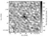 |
Fig. 1 Plateau de Bure Interferometer map (greyscale) of IFRS xFLS 478 at 105 GHz (2.9 mm) overlaid with the VLA 1.4 GHz radio contours from Condon et al. (2003), starting at 3σ and increasing by factors of 4. |
The CLEANed map is shown in Fig. 1.
Since the source appeared to be point-like in the CLEANed map, we fitted the uv data with the Fourier transform of a point source and found this fit to be consistent. Based on the fit, we obtained a flux density of 220 μJy beam-1 for xFLS 478 at 105 GHz. With a measured rms noise of 36 μJy beam-1, this corresponds to a 6.1σ detection. This is the highest-frequency detection of an IFRS in the radio regime. The absolute flux uncertainty is 10%.
2.7.3. Ancillary data of IFRS xFLS 478
Counterparts of xFLS 478 have been detected at 610 MHz (GMRT; Garn et al. 2007), 325 MHz (Westerbork Northern Sky Survey; Rengelink et al. 1997), and 151 MHz (6th Cambridge Survey; Hales et al. 1990). In the near- and mid-IR regime, xFLS 478 was observed with Spitzer and and detected at 4.5 μm, but remained undetected at 3.6 μm, 5.8 μm, and 8.0 μm (Lacy et al. 2005). Furthermore, the source xFLS 478 was observed by the Herschel Multi-tiered Extragalactic Survey (HerMES; Oliver et al. 2012) and was detected at 250 μm, 350 μm, and 500 μm. Source xFLS 478 remained undetected in the Sloan Digital Sky Survey data release 10 (SDSS DR10; Ahn et al. 2014) and also in the R band survey (50% completeness at 24.5 Vega mag; Fadda et al. 2004) with the Mosaic-1 camera on the Kitt Peak National Observatory. Hence, the redshift of this source is unknown.
3. Building and fitting the radio SEDs
Using the data presented in Sects. 2.1 and 2.2, we built radio SEDs for all 34 IFRS from our sample in CDFS and ELAIS-S1 based on all photometric detections and flux density upper limits. The resulting radio SEDs of three IFRS are shown in Fig. 2 and in Appendix B in Fig. B.1.
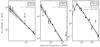 |
Fig. 2 Radio SEDs of three IFRS in CDFS, using all available flux density data points and upper limits. The solid line shows the fit which was found to best describe the photometric detections as discussed in Sect. 3. Spectral index and – if applicable – turnover frequency of the best fit are quoted. We also show the first approach to describe the data – a single power law fitted to all photometric detections – by a dotted line if this fit was discarded later in the analysis. 1σ uncertainties of the single power law fits are represented by the shaded areas. Error bars show 1σ uncertainties. The frequency coverage varies from one IFRS to another and the flux density scales are different. The radio SEDs of the other 31 IFRS studied in this paper are shown in Fig. B.1. |
-
1.
For each source, as the simplest approach, we fitted a single power law based on a least-squared method to all available photometric detections of the radio SED, weighting the data by their respective uncertainties. The ATLAS DR3 in-band spectral indices were not used in the entire fitting approach. The resulting fitted single power laws are shown in Fig. 2 and in Appendix B in Fig. B.1. We considered the fitted single power law as an appropriate description of the radio SED if (I) the low-frequency tail (below 1.4 GHz) and (II) the high-frequency (above 1.4 GHz) tail of the radio SED – considering detections and upper limits – were consistent with the fit, and (III) no turnover was seen in the central part of the radio SED. More precisely, for (I) and (II), we required that the cumulative low-frequency (high-frequency) deviation was below 1σ or the fractional low-frequency (high-frequency) deviation per data point was below 0.3σ.
-
2.
If the single power law in (1) was rejected because of (I) or (III), we fitted a radio SED model with a turnover to the photometric detections based on a least-squared method and weighting the data points by their uncertainties. The different models explaining this turnover can be divided by the location of the related physical process: internal or external to the synchrotron-emitting region (Kellermann 1966). If an external process is thought to cause the turnover, the physical process is expected to be free-free absorption by ionised gas outside the radio-emitting region. However, if the physical process is internal, synchrotron self-absorption (SSA) in the synchrotron-emitting region itself is usually assumed to cause the turnover. Since we found our data to trace only – if at all – the turnover in the radio SEDs but not the slope towards low frequencies (see Fig. 2 and Fig. B.1), we were not able to study the physical processes causing the turnover. Therefore, the decision which model to use for the fit was not relevant for our study and did not change our results. We decided to use an SSA model (e.g. Tingay & de Kool 2003) given by
 (2)where S0 denotes the zero flux density,
ν the
frequency, ν0 the frequency where the synchrotron
optical depth is equal to 1, β the power law index of the relativistic
electron energy distribution, and τν the
frequency-dependent optical depth. If the low-frequency end of the radio SED was
constrained by flux density upper limits and these limits were inconsistent with the
fitted single power law, we included these limits in the fitting to obtain a lower
limit on the peak frequency since lower flux densities at low frequencies will push
the peak towards higher frequencies. Sources fitted by the SSA model are discussed in
Sect. 4.6. The fitted SSA model is shown for
these sources in Fig. 2 and in Appendix B in Fig. B.1.
(2)where S0 denotes the zero flux density,
ν the
frequency, ν0 the frequency where the synchrotron
optical depth is equal to 1, β the power law index of the relativistic
electron energy distribution, and τν the
frequency-dependent optical depth. If the low-frequency end of the radio SED was
constrained by flux density upper limits and these limits were inconsistent with the
fitted single power law, we included these limits in the fitting to obtain a lower
limit on the peak frequency since lower flux densities at low frequencies will push
the peak towards higher frequencies. Sources fitted by the SSA model are discussed in
Sect. 4.6. The fitted SSA model is shown for
these sources in Fig. 2 and in Appendix B in Fig. B.1.
-
3.
Sources that were found to be poorly described by a single power law because of (II) can be divided in two subclasses, depending on the departure of the fitted power law from the SED:
-
(a)
If the highest frequency data points departed upwards from thefitted single power law, the source was considered as showing anupturn in the radio SED. A new single power law was then fitted tothe data of this source, while ignoring the deviatinghigh-frequency data points, and this fit is also shown inFig. 2 and in Fig. B.1. Thesesources are discussed in Sect. 4.5.
-
(b)
If high-frequency flux densities or upper limits were found to depart downwards from the fitted single power law, the source was considered to steepen towards higher frequencies. This subclass is discussed in Sect. 4.4.
-
(a)
The classification of each IFRS and the spectral index at the high-frequency side of the synchrotron bump – obtained from the best fit as described above – are summarised in Table 3.
Characteristics and results of our sample of 34 IFRS in ELAIS-S1 and CDFS.
Also listed is the IAU designation, the position, and the radio-to-IR flux density ratio from Zinn et al. (2011) or Maini et al. (2013). We do not quote reduced chi-squared numbers for the fits since upper limits were used as constraints in some cases as discussed above. A statistical comparison between the fits based on these numbers would be incorrect.
The SEDs of the sources in our control sample were built and fitted in the same way. We found the SEDs to be self-consistent, i.e. without spectral features that might arise from flux density measurements at different angular resolutions. Since the IFRS and control samples would suffer from the same effects, we are confident that our analysis is not significantly affected by changing resolution. In particular, we found that our approach to classify radio SEDs as described above works for the IFRS sample and for the control sample. In the subsequent analysis, we quote numbers for the control sample in square brackets.
The class of IFRS has not been studied with respect to radio variability. Therefore, variability effects on the radio SEDs presented here cannot be ruled out. In general, long-term variability (of the order of a year) of radio sources is low at 1.4 GHz and lower frequencies (e.g. Ofek & Frail 2011; Thyagarajan et al. 2011; Mooley et al. 2013). However, this is not necessarily the case at higher frequencies ≳5 GHz where a significant fraction – a few tens per cent – of sources show variability of the order of 10% or more (e.g. Bolton et al. 2006; Sadler et al. 2006; Franzen et al. 2009; Chen et al. 2013). In particular, flat- or inverted-spectrum radio sources are variable because of their dominating, beamed core emission (e.g. Franzen et al. 2014). These classes of object usually dominate samples selected at ~20 GHz. So it is very unlikely that the 1.4 GHz flux densities of our sample are significantly affected by variability, but we have no information about variability at higher frequencies.
4. Discussion: radio SEDs of IFRS
4.1. Sources following a single power law
Out of our sample of 34 IFRS [34 sources in the control sample], the SEDs of 23 IFRS [29 sources from the control sample] were well described by a single power law fitted to all available photometric data as described in Sect. 3. These sources do not show any evidence for a deviation from this fit, neither at low nor high frequencies. However, we note that nine [eight] of these sources are comparatively faint or are affected by confusion in some of the observations, reducing the number of photometric detections and, consequently, the number of data points constraining their radio SEDs. Therefore, we were able to exclude a deviation from the fitted single power law – by increasing or decreasing flux density at low or high frequencies – for only 14 of the 23 IFRS or  % [21 of the 29 sources in the control sample, or
  %] based on the available data.
Klamer et al. (2006) studied the radio SEDs of a sample of 37 HzRGs, selected at observed frequencies between 843 MHz and 1.4 GHz. The majority of their sources (89%) were found to be well described by a single power law in the studied frequency range between 843 MHz and 18 GHz. Our frequency coverage extends significantly to lower frequencies compared to theirs. If considering only the radio SEDs above 800 MHz, we found  % of our IFRS to be well described by a single power law, similar to the HzRG sample from Klamer et al.Emonts et al. (2011a,b) found three HzRGs to follow single power laws up to frequencies of 36 GHz. Out of the five IFRS with 34 GHz detections presented in our work, we find three to be consistent with a single power law up to 34 GHz, whereas the SEDs of the remaining two IFRS slightly steepen towards that frequency.
4.2. Radio spectral index
Based on the best fit found for each IFRS as described in Sect. 3, we found spectral indices between −0.52 and −1.39 [between −0.01 and −1.6] on the high-frequency side of the synchrotron bump for the 34 IFRS in our sample. The median index is −0.88 ± 0.04 [−0.74 ± 0.06] and the mean index is −0.91 ± 0.20 [−0.69 ± 0.29]. We emphasise that more high-frequency data is available for the IFRS sample than for the control sample. Therefore, numbers of the two samples cannot be compared.
Our median spectral index for IFRS of −0.88 is flatter than the median index of −1.4 for IFRS found by Middelberg et al. (2011). However, we measured the spectral index over a wider frequency range – particularly towards lower frequencies –, whereas the median index from Middelberg et al. has been measured between 1.4 GHz and 2.4 GHz. Middelberg et al. also find a spectral steepening towards higher frequencies which is discussed in detail in Sect. 4.4. They present a median spectral index for HzRGs of α = −1.02 between 1.4 GHz and 2.4 GHz which is close to the number found in our study for IFRS. Our median spectral index is steeper than the median spectral index of the entire radio source population (α = −0.74) and the AGN population (α = −0.63) in the ATLAS fields as presented by Zinn et al. (2012) between 1.4 GHz and 2.3 GHz. The median spectral index of the broader radio source population presented by Zinn et al. is consistent with the median spectral index of −0.74 found for our control sample.
We also studied the 1.4 GHz spectral indices from the ATLAS DR3 data. In contrast to the spectral indices obtained from a fit to the radio SED described above, these 1.4 GHz spectral indices are based on the same data for the IFRS sample and the control sample. Therefore, both samples can be properly compared based on the 1.4 GHz spectral indices. The histogram of these spectral indices is shown in Fig. 3.
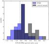 |
Fig. 3 Histogram of the ATLAS DR3 spectral indices |
We found that the IFRS sample has a steeper median radio SED than the control sample and that the spectral index distribution of IFRS is shifted towards steeper SEDs compared to the control sample, describing the broader, flux density-matched radio source population. The intrinsic difference between these two populations is also shown by a two-sample Anderson-Darling (A-D) test (Scholz & Stephens 1987). The A-D test measures the sum of the squared deviations of the samples and is more sensitive than a Kolmogorov-Smirnov (K-S), in particular at the tails of the distribution (Babu & Feigelson 2006). We rejected the null hypothesis that the spectral indices in the IFRS sample and in the control sample have the same parent distribution (probability p< 0.0015).
4.3. Ultra-steep, steep, flat, and inverted radio SEDs
The IFRS in our sample show generally steep radio SEDs. However, there is no generally accepted definition for steep and ultra-steep spectrum (USS) sources and selection criteria differ between studies with respect to frequencies and critical spectral index. Steep radio SEDs might be defined based on a spectral index α< −0.8. Following this criterion, 25 ( %) [7;
  %] out of 34 IFRS can be classified as steep-spectrum sources.
Afonso et al. (2011) point out that a significant number of sources with measured spectral indices steeper than a critical index are likely to be intrinsically flatter due to the long tail of the spectral index distribution. They argue that α< −1.0 is a reasonable definition for USS sources and used a conservative cut α< −1.3 between 610 MHz and 1.4 GHz for their sample. We found two IFRS ( %; CS538, ES1259) [1;
  %] in our sample with a spectral index steeper than −1.3. They are most likely to be USS sources. Further, six (
 %) [3;
  %] IFRS have a spectral index in the range −1.3 ≤ α ≤ −1.0. These sources are also good candidates for USS sources. In particular, we found statistically significantly more steep-spectrum sources in the IFRS sample than in the control sample. Based on a Fisher’s exact test (e.g. Wall & Jenkins 2012), we found a probability p< 0.001 that the subsets of sources with α< −0.8 in the IFRS and the control samples were obtained from the same parent spectral index distribution, consistent with the different ATLAS spectral index distributions presented in Sect. 4.2.
USS sources in IFRS samples were already found by Garn & Alexander (2008) who classify three ( %) IFRS in their sample as USS sources based on a spectral index α< −1 between 610 MHz and 1.4 GHz. Collier et al. (2014) find 155 (
 %) USS sources – defined by α ≲ −1.0 – in their all-sky sample of IFRS.
Steep-spectrum radio sources tend to be at higher redshifts (e.g. Tielens et al. 1979; McCarthy et al. 1991; Roettgering et al. 1994; Chambers et al. 1996; Klamer et al. 2006), although exceptions in both directions are known (see references in Afonso et al. 2011). The suggested high redshifts of IFRS – the highest known redshift is z = 2.99 (Collier et al. 2014) – have been confirmed based on optical spectroscopy (Collier et al. 2014; Herzog et al. 2014). However, it has been argued that the IR-faintest IFRS might be at even higher redshifts (Norris et al. 2011; Collier et al. 2014; Herzog et al. 2014). Our finding that the fraction of steep-spectrum sources is higher in the IFRS sample than in the control sample can be interpreted that IFRS might be at higher redshifts than ordinary RL AGN.
Two IFRS from our sample have spectroscopic redshifts: CS265 (z = 1.84) and CS713 (z = 2.13). They are among the IR and optically brightest IFRS in the ATLAS fields and are therefore expected to be at the lower tail of the redshift distribution of IFRS. Following the connection between steepness of the radio SED and redshift, the radio spectral indices for these sources presented in this work of −0.84 and −0.56 – lower than the median spectral index – suggest that these sources have lower redshifts than the median IFRS in our sample, consistent with the argument based on the IR flux densities.
We found two (%) IFRS in our sample [10;  %] with a flat (−0.6 ≤ α ≤ 0) and none (0+ 5%) [0; 0+ 5%] with an inverted (α> 0) radio SED. Based on these numbers, we are confident that the radio SEDs presented in this work are not significantly affected by radio variability as discussed in Sect. 3.
4.4. Radio SEDs steepening towards higher frequencies
We found five IFRS ( %; CS164, ES427, ES509, ES798, ES973) [one; %] in our sample that show a steepening radio SED towards higher frequencies, suggesting that a single power law does not properly describe the data. This spectral behaviour was already found for two of these IFRS by Middelberg et al. (2011) and can be explained by a recently inactive AGN. In a magnetic field, higher-energy electrons lose their energy faster than low-energy electrons. If a region of synchrotron emission is not fed by the continuous injection of new particles, the highest-energy particles are cooled quicker by energy losses than low-energy particles, resulting in a lack of radiated high-energy photons and a steepening in the SED towards higher frequencies (e.g. Kardashev 1962).
Middelberg et al. (2011) matched the uv coverage of their observations at 4.8 GHz and 8.6 GHz to eliminate the possibility that the observed spectral steepening between 4.8 GHz and 8.6 GHz might be caused by resolution effects. Therefore, this can be ruled out for ES798 and ES973 – both detected at 4.8 GHz but undetected at 8.6 GHz – and CS164 which was detected at both frequencies.
Based on their resolution-matched spectral indices between 1.4 GHz and 2.4 GHz on the one hand and between 4.8 GHz and 8.6 GHz on the other hand, Middelberg et al. (2011) find that the radio SEDs of IFRS generally steepen towards higher frequencies. Some IFRS in our sample are also steepening towards higher frequencies. However, our data at high frequencies are generally not sensitive enough to detect or constrain the radio SED of our IFRS. Only four IFRS were detected in the higher-frequency surveys by Huynh et al. (2012) and Franzen et al. (2014); these are the only IFRS from our sample detected at a frequency above 2.3 GHz that were not covered in the observations by Middelberg et al. For these four sources, we did not find evidence for a steepening. In contrast, one of those four IFRS even shows an upturn as discussed in the following Sect. 4.5.
We found a steepening radio SED towards higher frequencies for only one source in our control sample. However, few high-frequency data are available in the control sample since the observations at 4.8 GHz, 8.6 GHz, and 34 GHz were targeted observations of IFRS and no data are available at these frequencies for the sources in the control sample. Therefore, we cannot exclude the possibility that a steepening occurs for some of the control sources but is not seen in our data because of poor high-frequency coverage and sensitivity. Klamer et al. (2006) did not find any HzRG in their sample of 37 sources that steepens at higher frequencies. If the fraction of steepening sources is higher for IFRS than for HzRGs, this might suggest an intrinsic difference. In that case, IFRS might be recently inactive and restarted RL AGN, whereas HzRGs do not show any evidence for a changing activity of their active nucleus.
4.5. IFRS with an upturn in their radio SED
The radio SED of IFRS CS603 follows a single power law in the frequency range between 800 MHz and 10 GHz. At higher frequencies, however, the SED departs from this power law, showing an increasing flux density with increasing frequency. This is indicated by the 18 GHz detection and clearly visible from the 20 GHz detection. There are two potential explanations for this behaviour.
A flattening or upturning SED at high frequencies can be explained by a flat or inverted SED of an AGN core that is dominating over the steep synchrotron SED of the lobes at these frequencies. Alternatively, the upturn might be caused by dust. It is known that thermal free-free and dust emission start to dominate over the non-thermal synchrotron emission at rest-frame frequencies above ~100 GHz in starburst galaxies (e.g. Murphy 2009; Fig. 2), though thermal dust emission significantly depends on the size and composition of the dust grains. Considering that IFRS are known to be AGN and that no evidence for heavy dust obscuration in IFRS has been found (Collier et al. 2014), the flat or inverted radio SED of an AGN core seems to be the most plausible explanation. This interpretation is consistent with results from Hogan et al. (2015a,b), who find that a fainter, flatter spectral core component is often present in the radio SEDs of brightest cluster galaxies (BCGs). However, higher-frequency observations of IFRS CS603 are needed to add evidence to this hypothesis.
Since we found an upturning SED at high frequencies also for one source in the control sample, this spectral behaviour does not seem to be a characteristic feature of IFRS, but to occur in the broader RL AGN population, too. The results from Klamer et al. (2006), finding 11% of their HzRGs flattening at higher frequencies, is also consistent. The putative causes for this effect discussed with respect to the IFRS are also valid for HzRGs and ordinary AGN without IR-faintness.
4.6. Radio SEDs showing a turnover
Covering the frequency regime between 200 MHz and 34 GHz in ELAIS-S1 and between 150 MHz and 34 GHz in CDFS, our data enabled us to detect the turnover in the radio SEDs of IFRS in a wide frequency range. In particular, GPS sources with a turnover frequency above 500 MHz and CSS sources, peaking at frequencies below 500 MHz, should be detectable based on our rich data set. It has been argued by Middelberg et al. (2011) and Herzog et al. (2015a) that an overlap between the population of GPS and CSS on the one hand and IFRS on the other hand might exist. Collier et al. (2014) find that at least a few IFRS are GPS or CSS sources.
The radio SEDs shown in Fig. 2 and Fig. B.1 revealed that CS164, ES509, and ES1156 have a turnover in the frequency range of a few hundred MHz (three sources in the control sample). Based on fitting an SSA model to the data, we found peak frequencies in the observed frame between 130 MHz and 680 MHz [200 MHz – 1.1 GHz]. In addition to these three IFRS, the radio SEDs of CS114, CS538, and CS649 (no source) also suggest a turnover in the frequency regime covered by our data. However, the putative peak in the radio SEDs of these three sources is indicated only by flux density upper limits. Based on fitting the SSA model to the flux density upper limits, we obtained lower limits of the peak frequencies between 200 MHz and 320 MHz for these three sources.
Summarising, we found six (%) IFRS [3; %] in our sample of 34 sources that show a clear turnover in their radio SED based on photometric detections or flux density upper limits. Out of these peaking sources, one IFRS [one] was found to peak at an observed frequency above 500 MHz, fulfilling the selection criterion of GPS sources (note that GPS sources are usually defined based on their observed peak frequency; O’Dea 1998). Based on these numbers, we suggest that % of IFRS [%] are GPS sources. Considering that we cannot rule out a turnover in the frequency range above 200 MHz for nine [eight] other sources since their low-frequency regime is only constrained by upper limits, we conclude that between % and  % of IFRS [between % and
  %] show a turnover at a frequency above ~150 MHz. However, since CSS sources can also have their turnover at frequencies below 150 MHz – i.e. even IFRS following a single power law down to 150 MHz might be CSS sources –, we are not able to set an upper limit on the fractional overlap between IFRS and CSS sources. However, we suggest that this overlap is ≥% [≥
 %]. The class of CSS sources (e.g. O’Dea 1998) is defined by steep radio SEDs (α ≲ −0.5) and compact morphology (a few or a few tens of kpc). Since IFRS are known to be compact with linear sizes of not more than a few tens of kpc (e.g. Garn & Alexander 2008; Middelberg et al. 2011) and to have steep radio SEDs (Middelberg et al. 2011; and discussion in Sects. 4.2 and 4.3), IFRS are prototypical for the class of CSS sources. In particular, we found five additional sources (CS415, CS539, ES66, ES427, and ES645) that slightly departed from the fitted single power law or flattened at low frequencies and might be CSS sources not represented in our statistics. Therefore, we suggest that the fraction of CSS sources is putatively significantly higher than the observed fraction of %.
In our control sample, we found % and ≥% of the sources to be GPS sources and CSS sources, respectively. Considering that the latter number is a lower limit, these numbers are consistent with those found by O’Dea (1998) in the broader population of RL AGN (~10% and ~30%, respectively). Comparing these numbers to those found for our IFRS sample, we did not find evidence for a higher fraction of GPS and CSS compared to samples of ordinary RL AGN. However, the potentially high redshifts of our IFRS sample might prevent us from tracing the expected peak in the radio SED covered by our data. Although suffering from small number statistics, the lower turnover frequencies found in the IFRS sample compared to the control sample is consistent with putatively higher redshifts of IFRS.
When comparing samples selected at different frequencies, selection biases have to be taken into account. Generally, the selection frequencies affect the number of detected sources in the respective samples. When comparing the fractions of GPS sources, an additional selection bias is present. Since the low-frequency slope in the radio SED of a GPS source is usually steeper than the high-frequency slope, a sample selected at 1.4 GHz is more likely to find sources peaking at lower frequencies than samples selected at higher frequencies like the Tenth Cambridge (10C) survey of radio sources (AMI Consortium et al. 2011a,b; Whittam et al. 2015) at 15.7 GHz or the AT20G (Murphy et al. 2010; Franzen et al. 2014) survey at 20 GHz. This provides a potential explanation both for the lower GPS fraction in our sample compared to the sample presented by O’Dea (1998) – mainly selected at 5 GHz – and for the finding that the few GPS sources in our sample are peaking at relatively low frequencies.
It has already been argued that a significant fraction of IFRS might be young AGN in their earliest evolutionary stages (Collier et al. 2014; Herzog et al. 2015a). Although our results based on the turnover do not provide evidence for a higher fraction of GPS and CSS sources in the IFRS population, they do not exclude this possibility either. Instead, a high fraction of CSS sources is likely because of the steep radio SEDs and the compact morphology of IFRS. If IFRS are indeed younger – i.e. with turnovers at high rest-frame frequencies – and at higher redshifts than the broader AGN population, these two effects would work against each other. A younger radio galaxy is expected to peak at a higher rest-frame frequency, but a high redshift shifts this peak to a lower frequency, resulting in similar observed fractions of GPS and CSS sources in the IFRS population and in the broader RL AGN population. Since we are lacking redshifts for the vast majority of IFRS in our sample, we are unable to distinguish between these two effects contributing to the observed peak frequency: evolution of the AGN, and cosmology.
4.7. Connection between turnover frequency and linear size
Based on samples of GPS and CSS sources, O’Dea & Baum (1997) presents an anti-correlation between intrinsic turnover frequency and linear size (their Fig. 3). In the evolutionary scenario for AGN described in Sect. 4.6, this correlation implies a shift of the turnover to lower frequencies while the AGN evolves and the jets expand. Here, we analyse our sample in the context of this scenario.
The typical linear size of fully evolved RL AGN, i.e. FRI/FRII, is around 100 kpc or higher (Pentericci et al. 2000). Higher resolution data used in our work show that the majority of IFRS are smaller than 100 kpc as already mentioned by Garn & Alexander (2008) and Middelberg et al. (2011). However, generally, the angular resolution of our observational data is not high enough to test whether the correlation between intrinsic turnover frequency and linear size holds for our sources. The plot from O’Dea & Baum (1997) shows sources with linear sizes of around 10 kpc and smaller. Furthermore, the two correlated quantities are redshift-dependent, resulting in an additional uncertainty for the redshift-lacking IFRS sample.
Even for the most compact IFRS, the correlation from O’Dea & Baum (1997) provides only weak constraints. Middelberg et al. (2011) concluded that three IFRS (CS703, ES427, ES509) are even smaller than 4.5 kpc × 2.1 kpc since they do not show any evidence for being resolved at any of the five frequencies used in their study. Following O’Dea & Baum, a source limited to that linear size is expected to show a turnover at a rest-frame frequency of around 300 MHz or higher. Already at a redshift of z = 1.5, this turnover would have been shifted out of the frequency range covered by our data. This is consistent with our finding, that the radio SEDs of CS703 and ES427 clearly follow single power laws down to observed frequencies of 100 MHz without indicating a turnover. In contrast, the radio SED of ES509 shows a turnover at an observed frequency of around 130 MHz. Assuming a rest-frame peak frequency of at least 300 MHz following from the O’Dea & Baum correlation, this IFRS is expected to be at a redshift z ≳ 1.5.
Going the other way around and using the fitted peak frequencies of 370 MHz and 680 MHz for ES1156 and CS164, the rest-frame peak frequencies are above 1 GHz and 2 GHz, respectively, assuming that these sources are at z ≳ 2. Following the correlation presented by O’Dea & Baum (1997), these objects are expected to be smaller than ~300 pc and ~100 pc, respectively. In all available maps, CS164 and ES1156 were found to be very compact. In particular, CS164 was observed by Middelberg et al. (2011) at high angular resolution and did not reveal any substructure, suggesting an angular size of less than 1 arcsec, consistent with the linear size estimated from the observed turnover frequency.
Middelberg et al. (2011) find IFRS ES509 to be very compact and suggest an angular size of less than 0.9 × 0.3 arcsec2, corresponding to a physical size of 8 × 3 kpc2 for z ~ 1.5. The O’Dea & Baum (1997) correlation suggests an intrinsic turnover frequency of 100 MHz to 300 MHz, consistent with the observed turnover frequency of 130 MHz for ES509 discussed above.
4.8. Spectral components in the radio SED of IFRS
The radio SED of an AGN may consist of one or more components. The core component, mainly contributing at higher frequencies and potentially showing a peak in the SED arising from SSA, is expected to represent the most recent activity of the central engine and to be more time-variable than the steep spectrum component of the extended emission. The latter – mainly given by the lobes – represents the interaction between jet and the ambient medium and therefore traces past activity of the core, with fading time scales of 104−5 yrs (Miley & De Breuck 2008). In contrast, the core component is expected to fade on timescales of the order of 101−3 yrs (O’Dea & Baum 1997; de Vries et al. 2010). Since the contributions of the individual components to the total SED are changing with time because of these different fading timescales, analysing the total radio SED for individual spectral components provides a tool to study the activity status of the AGN. Since the core components are likely to correspond to rest-frame frequencies of a few tens of GHz, it is important that these high frequencies are considered when studying radio sources even at low redshifts.
Our radio SED analysis showed that both components are found in the SEDs of IFRS as presented in Sects. 4.1, 4.5, and 4.6. For example, it might be suggested that the core of CS603 has been active more recently than that of e.g. CS703 because of the additional – putatively inverted – spectral component at high frequencies. In contrast, the core of CS164 might still be active since the core component is dominating the total radio SED which is that of a GPS source. Our finding that seven out of 34 IFRS in our sample are showing evidence for a core component – all sources discussed in Sects. 4.5 and 4.6 – is consistent with the fraction of IFRS with a detected VLBI core. In addition, the radio SED of IFRS ES749 points at an additional radio component at an observed frequency of around 200 MHz. A similar behaviour might be found in the radio SEDs of ES1018 and ES1259, but the frequency coverage is not dense enough to substantiate this hypothesis. Importantly, a source found to be consistent with a single power law up to 20 GHz like CS703 might still have a flat or peaked spectrum component at higher frequencies.
4.9. Radio spectral index as a function of IR and radio properties
So far, we have focused on the radio SEDs of our IFRS sample and found that the population of IFRS does not necessarily deviate from the general RL source population with respect to the fraction of GPS and CSS sources. However, IFRS were found to have steeper radio SEDs than the ordinary AGN and star forming galaxy populations. Here, we link the radio SEDs to the IR properties of IFRS.
As discussed in Sect. 4.4, higher-redshift radio galaxies have generally steeper radio SEDs. Connecting this correlation to the suggested relation between 3.6 μm flux density and redshift for IFRS (Norris et al. 2011; Collier et al. 2014; Herzog et al. 2014), IR-fainter IFRS would be expected to have steeper radio SEDs. We tested our data for this potential correlation and show the spectral index as a function of 3.6 μm flux density in Fig. 4 (top left).
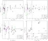 |
Fig. 4 Radio spectral index α as a function of the 3.6 μm flux density (top left), α as a function of the radio flux density S1.4 GHz (top right), α as a function of the radio-to-IR flux density ratio S1.4 GHz/S3.6 μm (bottom left), and S1.4 GHz/S3.6 μm as a function of S1.4 GHz (bottom right) for our sample of 34 IFRS. The symbols distinguish subsamples of different turnover properties. Green dots represent sources with a detected turnover. Sources with a possible peak are shown by purple squares, and sources without a peak by black crosses. The classification is described in Sect. 3 and summarised for individual IFRS in Table 3. Upper and lower limits are represented by arrows. The grey horizontal and vertical lines indicate the medians or limits of the median. |
Our data provide statistically significant evidence for a correlation between IR flux density and spectral index. When splitting our sample at a 3.6 μm flux density of 15 μJy, we found only one ( %) out of eight IFRS in the IR-brighter subsample with a radio SED steeper than the median, whereas 15 (
 %) out of 26 IFRS in the IR-fainter subsample have a steeper spectral index than the median. We also tested the data based on a Spearman rank correlation test (e.g. Wall & Jenkins 2012) and found a correlation coefficient r between 0.29 and 0.61, considering the unknown relation between the IR-undetected sources. A coefficient of 1 (−1) corresponds to an ideal (anti-)correlation, whereas 0 indicates a lacking correlation. The probability p that 3.6 μm flux density and spectral index are uncorrelated is between 0.046 and 0.00005. Therefore, we reject the hypothesis that 3.6 μm flux density and radio spectral index are uncorrelated at a 0.05 significance level. For the control sample, we found a correlation coefficient of 0.14, indicating no evidence of a strong correlation.
We also looked at the spectral index as a function of 1.4 GHz flux density as shown in Fig. 4 (top right) and found no correlation, neither in the IFRS nor in the control sample. Based on 15.7 GHz data, Franzen et al. (2014) showed that the general radio source population with 15.7 GHz flux densities above ~25 mJy and below ~1 mJy is dominated by flat (α> −0.5) spectrum sources, whereas the intermediate flux density range is dominated by sources with steep (α< −0.5) radio SEDs. We did not find any dependence at 1.4 GHz. However, our sample has been selected at lower frequencies and our sample covers only one order of magnitude in 1.4 GHz flux density, in contrast to the sample by Franzen et al.
The bottom left plot of Fig. 4 shows the spectral index α as a function of the radio-to-IR flux density ratio S1.4 GHz/S3.6 μm. We find a Spearman rank correlation coefficient between −0.20 and −0.63 and a probability between 0.12 and 3 × 10⁻⁵ that both quantities are uncorrelated, pointing at a potential anti-correlation between spectral index and radio-to-IR flux density ratio.
4.10. Comparison of peaking and non-peaking sources
As presented above, we found six IFRS that show a turnover in their radio SEDs and 19 IFRS unambiguously without a peak in the frequency range covered by our data. These subsamples are clearly marked in Fig. 4, showing the IFRS sample in the parameter spaces of spectral index, radio flux density, IR flux density, and radio-to-IR flux density ratio. We find that five out of the six peaking IFRS have 3.6 μm flux densities of 3 μJy and lower, below the median of the entire IFRS sample. In contrast, these six peaking IFRS have 1.4 GHz flux densities from the entire flux density range covered by the total IFRS sample. Similarly, the radio-to-IR flux density ratios of the IFRS with a turnover in their radio SED do not differ from those of the non-peaking subsample.
Our subsample of peaking sources putatively contains GPS and young CSS sources, whereas the non-peaking subsample is expected to contain older CSS sources peaking at observed frequencies below 150 MHz. Since we found the peaking subsample to be IR-fainter, we expect these IFRS to be at higher redshifts, following the suggested correlation between 3.6 μm flux density and redshift for IFRS (Norris et al. 2011; Collier et al. 2014; Herzog et al. 2014). On the other hand, the IR faintness and expected higher redshifts of the peaking subsample make a detection of the peak less likely since the turnover would be redshifted out of the frequency regime covered by our data. Redshift information is crucial to disentangle these two effects – evolution and cosmology –, contributing in opposite directions.
4.11. Radio SED of IFRS CS618
The IFRS CS618 is peculiar and has a different morphology than any other source in our IFRS sample. The 3.6 μm map of CS618 overplotted by the 1.4 GHz ATLAS DR3 contours is shown in Fig. 5.
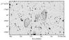 |
Fig. 5 3.6 μm SWIRE map (Lonsdale et al. 2003; greyscale) of CS618 overplotted by the 1.4 GHz ATLAS DR3 (Franzen et al. 2015) contours. Contours start at 3σ and increase by factors of 4. CS618 is an evolved FRII radio galaxy with an unresolved core (centre of the shown map) and two slightly resolved lobes. |
It appears as a double-lobed FRII radio galaxy with an angular size of around 1.7 arcmin. Its total radio SED (containing the core and the two lobes) is well described by a single power law with a spectral index α = −1.06 ± 0.05 (see Fig. B.1). All three components are separately detected at 325 MHz, 610 MHz, 1.4 GHz and 2.3 GHz, but are indistinguishable at 200 MHz, 843 MHz, and 844 MHz because of the lower resolution. The radio SEDs of all three individual components are well described by single power laws. The central component (1.6 mJy at 1.4 GHz) is unresolved with a spectral index between 325 MHz and 2.3 GHz of +0.33 ± 0.17, whereas the two lobes are slightly resolved with 1.4 GHz flux densities of 34.5 mJy and 11.4 mJy, and spectral indices between 150 MHz and 2.3 GHz of −1.01 ± 0.09 and −1.23 ± 0.13. These characteristics are common for FRII radio galaxies (e.g. Hovatta et al. 2014) and so CS618 seems to differ from the majority of IFRS in our sample, which are dominated by more compact and putatively younger radio sources as discussed above.
4.12. Comparison to sources used in broad-band SED modellings
Herzog et al. (2014) presented the first redshift-based SED modelling of IFRS and find all three studied IFRS in agreement with scaled templates of 3C 48 and 3C 273. Two of these three IFRS are also in our sample: CS265 and CS713. The radio SEDs of these IFRS were found to be in good agreement with single power laws with spectral indices of −0.84 ± 0.01 and −0.56 ± 0.04, respectively. 3C 48 is a CSS source with a spectral index of α ~ −0.8, and the core of the RL quasar 3C 273 is known to have a flat radio SED. Based on the spectral index found in our work, the core of 3C 273 seems to provide an inadequate template to explain the characteristics of IFRS CS265. In contrast, the spectral index of CS713 matches the flat radio SED known for 3C 273, whereas the steeper SED of 3C 48 disagrees with the characteristics of CS713.
An extended sample of SED templates was used by Herzog et al. (2015b) to constrain the broad-band SED of six IFRS observed with Herschel. All sources are also in our radio sample of IFRS and we found radio spectral indices between −0.92 and −1.08, i.e. all have steep or ultra-steep SEDs. Herzog et al. find only the redshifted broad-band SED templates of the spiderweb galaxy, Cygnus A, 3C 48, and 3C 273 to be in agreement with the data, even if the templates were scaled in luminosity and extinction was added. The flat radio SED of the core of 3C 273 is in clear disagreement with the steep radio SEDs found for all six sources. Also the radio SED of 3C 48 is flatter than any radio SED in that sample of six IFRS, although an overlap with the flattest sources in the IFRS sample cannot be ruled out. In contrast, both the spiderweb galaxy and Cygnus A are known to have ultra-steep radio SEDs with spectral indices of around −1.3 and −1.2, respectively. Thus, the radio spectral indices measured in our work add evidence to the conclusion presented by Herzog et al. that the spiderweb galaxy and Cygnus A provide adequate templates to explain the broad-band characteristics of IFRS.
5. The radio and multi-wavelength SED of IFRS xFLS 478
In Sect. 4, we analysed the broad radio SEDs of a large sample of IFRS in the ELAIS-S1 and CDFS fields. To complement this study, we present the detailed analysis of one IFRS (xFLS 478) in the following. This study is not limited to the radio regime, but also links to the far-IR (FIR) detections of this source. IFRS xFLS 478 is particularly suitable for this study since it provides the highest-frequency radio data point of an IFRS (at 105 GHz as presented in Sect. 2.7.2) and ancillary data in the radio and IR regime, described in Sect. 2.7.3.
Figure 6 shows the radio SED of this source – including all available data between 150 MHz and 105 GHz –, similar to the SEDs shown in Fig. 2 and in Appendix B in Fig. B.1.
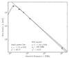 |
Fig. 6 Radio SED of IFRS xFLS 478. Error bars represent 1σ uncertainties. The black solid line shows the best fit of an SSA model. The fitted single power law is shown as black dotted line. The shaded area represents the 1σ uncertainty of the single power law fit. |
To describe the radio emission over this wide frequency range of almost three orders of magnitude, we followed the same approach as described in Sect. 3. Fitting a single power law to the data resulted in a spectral index α = −1.14 ± 0.02. However, the low-frequency data at 150 MHz and 325 MHz depart from the single power law, indicating a potential turnover. An SSA model was found to better describe the data, resulting in a turnover at 180 MHz and a spectral index of −1.19 ± 0.06 at the high-frequency side of the synchrotron bump. However, a turnover can only be suggested based on the available data; its frequency remains unclear. In any case, IFRS xFLS 478 has a steep radio SED and might – depending on the definition as discussed in Sect. 4.3 – be classified as a USS source according to both fits.
If the radio SED of xFLS 478 indeed follows the fitted single power law or the SSA model up to an observed frequency above 100 GHz, this provides interesting new constraints on the properties of IFRS. As shown by Collier et al. (2014) and Herzog et al. (2014), all known redshifts of IFRS are in the range 1.7 ≲ z ≲ 3.0. Assuming that xFLS 478 is at a similar redshift, the observed 105 GHz detection is at a rest-frame frequency ~300 GHz. It is known that the thermal free-free and dust emission in star forming galaxies start to dominate over non-thermal synchrotron emission at around 100 GHz (e.g. Murphy 2009) as discussed in Sect. 4.5. This would imply for xFLS 478 that the AGN emission of this source dominates over the emission from star forming activity even in the mm regime despite the Herschel detection at 250 μm. The alternative explanation for a flattening of the radio SED at higher frequencies – a dominating AGN core as discussed in Sects. 4.5 and 4.8 – can also be excluded for xFLS 478 up to this frequency. However, an additional, flat radio SED component might still start to dominate at higher frequencies as discussed above.
The same behaviour – following a power law up to the mm regime – was found for the source F00183-7111 (Norris et al. 2012), referred to as 00183. 00183 is one of the most luminous ULIRGs, being heavily obscured and undergoing vigorous star forming activity, at z = 0.3276. In VLBI observations, a core-jet structure was found in its centre with an extension of only 1.7 kpc, however the source is radio-loud. Norris et al. suggested that this source is undergoing a transition from a merging starburst with a quasar-mode AGN in its centre to an RL quasar. Emonts et al. (2011a,b) found three HzRGs to follow single power laws up to 36 GHz (115 GHz in the restframe).
We emphasise that while the suggested single power law or SSA model for xFLS 478 are the simplest explanation, it is based on only one detection in the mm regime. Other interpretations are also possible, such as a steepening SED above 1.4 GHz, followed by a minimum between 10 GHz and 100 GHz, and increasing thermal dust emission – dominating over synchrotron emission – at 105 GHz. Further high-frequency observations would be required to distinguish between these hypotheses In Sect. 4.5, we presented one IFRS that did not follow a power law up to high frequencies but showed deviations at observed frequencies around 20 GHz. Most likely, this deviation is caused by the flat or inverted SED of an AGN core.
We now consider the multi-wavelength SED of IFRS xFLS 478, including all ancillary data presented in Sect. 2.7.3 and following the approach used by Herzog et al. (2015b). In this modelling, SED templates of different galaxy classes typically found at high redshifts – including star forming galaxies with and without AGN, Seyfert galaxies, and RL AGN – were used, shifted in the redshift range 0.5 ≤ z ≤ 12, scaled in luminosity, and obscured by additional dust. These templates were then tested whether they are consistent with the photometric data of IFRS. In this comprehensive approach, we did not find any SED template that could reproduce the characteristics of IFRS xFLS 478 in the redshift regime 0.5 ≤ z ≤ 12. In particular, the most promising templates – RL AGN at high redshifts, e.g. HzRGs – were found to be inconsistent with the FIR detections of xFLS 478. Herzog et al. (2015b) observed six IFRS with Herschel that are only slightly radio-fainter than xFLS 478 but none was detected; the detection sensitivities were similar to the observed FIR flux densities of xFLS 478.
Consequently, we asked the question what properties a galaxy would need to have to be consistent with the photometric constraints of xFLS 478. To account for the HerMES FIR detections with flux densities of a few tens of mJy, we used the radio-FIR SED template of a star forming galaxy from Murphy (2009). This template is composed of synchrotron, free-free, and thermal dust components as shown in Fig. 7 for z = 1.1. However, the observed radio emission of xFLS 478 cannot be explained by star foming activity at any redshift. Therefore, we added the radio emission from an RL AGN, consistent with the finding that the majority of IFRS – if not all – contain AGN (Herzog et al. 2015a). We used the radio SED of 00183 from Norris et al. (2012). This source is known to host an RL AGN and to show similarities to xFLS 478 as discussed above. We shifted these templates in the redshift range 0.5 ≤ z ≤ 8.0 and built the total SED by summing both individual templates, each of them scaled by an individual factor. The best modelling was found at z = 1.1 and is shown in Fig. 7.
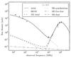 |
Fig. 7 Modelling the radio-FIR SED of IFRS xFLS 478. The total SED (solid line) is composed of the SED of a star forming galaxy (dashed line) from Murphy (2009) and the radio SED of 00183 (dotted line) from Norris et al. (2012). The star forming SED template is again composed of synchrotron, free-free, and thermal dust components. The best model was found at z = 1.1 and is shown in this figure. Black dots represent the photometric data points of xFLS 478 with respective 1σ uncertainties. |
We note that the fractional contributions from synchrotron, free-free, and thermal dust emission to the star forming galaxy template were fixed as described by Murphy and were not varied in our modelling.
The photometric data of the IFRS are well described by the model at z = 1.1, particularly in the FIR and mm regimes. The radio SED of xFLS 478 seems to be flatter at higher frequencies than that of 00183. Norris et al. (2012) fitted a broken power law to the radio SED of 00183, finding a break at around 5 GHz and spectral indices of −0.43 and −1.49 at low and high frequencies, respectively. We measured a spectral index of −1.19 for xFLS 478 as described above and did not find clear evidence for a break at higher frequencies.
At z = 1.1, the 00183 radio template had to be scaled up in luminosity by a factor of 3.0. The star forming galaxy template had to be scaled up by a factor of 1.9, giving a star formation rate of around 170 M⊙ yr-1. This model, if confirmed, makes xFLS 478 the lowest-redshift IFRS known.
6. Conclusion
We built radio SEDs for 34 IFRS in the CDFS and ELAIS-S1 fields, covering the frequency range between 150 MHz and 34 GHz. Based on these SEDs, we found the vast majority of IFRS (%) to show steep radio SEDs defined by α< −0.8. % of the IFRS in our sample are classified as USS sources (α< −1.3) and are therefore good candidates for high-redshift sources. The sample of IFRS shows statistically significantly steeper radio SEDs than the broader RL AGN population. The median spectral index in our IFRS sample is −0.88. One IFRS was found to show a flattening or upturning radio SED at 20 GHz, indicating an additional core component and emphasising the importance of considering high-frequency radio data when studying radio sources, irrespective of their redshift. Our finding that IR-fainter IFRS have steeper radio SEDs supports the hypothesis that IR-fainter IFRS are at higher redshifts.
We found % of our sample are GPS sources and ≥% are CSS sources. These numbers are consistent with the general fraction of GPS and CSS sources in the RL AGN population. This finding implies that at least some IFRS are young AGN in the earliest stages of their evolution to powerful and extended FRI/FRII radio galaxies. However, the intrinsic fraction of GPS and CSS sources in the IFRS population might be higher than in the general RL source population if IFRS are at higher redshifts. Generally, IFRS are prototypical for the class of CSS sources because of their steep radio SEDs and their compactness. Our analysis showed that IFRS with an observed peak in their radio SED are IR-fainter than IFRS without a turnover. However, we do not find evidence that the radio flux densities or the radio-to-IR flux density ratios of peaking IFRS differ from those of the non-peaking subsample.
We also carried out a detailed analysis of the broadband SED of IFRS xFLS 478. This source was observed with the PdBI at 105 GHz and provided the highest-frequency radio detection of an IFRS. The source was found to have a steep radio SED, potentially indicating a turnover at around 150 MHz. We did not observe an upturn or flattening in the radio SED at high frequencies, indicating that synchrotron emission dominates over thermal dust emission at least down to a rest-frame frequency of 300 GHz (1 mm) if the source is at z ≳ 2.
Modified SED templates of known galaxies were found to be inconsistent with the multi-wavelength data of xFLS 478. However, the data are well described by a radio-FIR SED template composed of a star forming galaxy and an RL AGN at z = 1.1 which would make this object the IFRS with the lowest known redshift. This model suggests a star formation rate of around 170 M⊙ yr-1.
JMFIT is a task of the Astronomical Image and Processing System (AIPS); http://www.aips.nrao.edu/
Acknowledgments
We thank our referee Alastair Edge for valuable suggestions which helped to improve this paper. We thank the IRAM staff for carrying out the PdBI observations and helping with data calibration. N.S. is the recipient of an ARC Future Fellowship. B.E. acknowledges funding through the European Union FP7 IEF grant No. 624351. This research has made use of the NASA/IPAC Extragalactic Database (NED) which is operated by the Jet Propulsion Laboratory, California Institute of Technology, under contract with the National Aeronautics and Space Administration. This research has made use of data from HerMES project (http://hermes.sussex.ac.uk/). HerMES is a Herschel Key Programme utilising Guaranteed Time from the SPIRE instrument team, ESAC scientists and a mission scientist. The HerMES data was accessed through the Herschel Database in Marseille (HeDaM – http://hedam.lam.fr) operated by CeSAM and hosted by the Laboratoire d’Astrophysique de Marseille.
The Australian SKA Pathfinder is part of the Australia Telescope National Facility which is funded by the Commonwealth of Australia for operation as a National Facility managed by CSIRO. This scientific work uses data obtained from the Murchison Radio-astronomy Observatory (MRO), which is jointly funded by the Commonwealth Government of Australia and State Government of Western Australia. The MRO is managed by the CSIRO, who also provide operational support to ASKAP. We acknowledge the Wajarri Yamatji people as the traditional owners of the Observatory site. The work was supported by iVEC through the use of advanced computing resources at the Pawsey Advanced Supercomputing Centre. Support for the operation of the MWA is provided by the Australian Government (NCRIS), under a contract to Curtin University administered by Astronomy Australia Limited. We acknowledge the Pawsey Supercomputing Centre which is supported by the Western Australian and Australian Governments.
References
- Afonso, J., Bizzocchi, L., Ibar, E., et al. 2011, ApJ, 743, 122 [NASA ADS] [CrossRef] [Google Scholar]
- Ahn, C. P., Alexandroff, R., Allen de Prieto, C., et al. 2014, ApJS, 211, 17 [NASA ADS] [CrossRef] [Google Scholar]
- Babu, G. J., & Feigelson, E. D. 2006, in Astronomical Data Analysis Software and Systems XV, eds. C. Gabriel, C. Arviset, D. Ponz, & S. Enrique, ASP Conf. Ser., 351, 127 [Google Scholar]
- Banfield, J. K., George, S. J., Taylor, A. R., et al. 2011, ApJ, 733, 69 [NASA ADS] [CrossRef] [Google Scholar]
- Bock, D. C.-J., Large, M. I., & Sadler, E. M. 1999, AJ, 117, 1578 [NASA ADS] [CrossRef] [Google Scholar]
- Bolton, R. C., Chandler, C. J., Cotter, G., et al. 2006, MNRAS, 370, 1556 [NASA ADS] [CrossRef] [Google Scholar]
- Cameron, E. 2011, PASA, 28, 128 [NASA ADS] [CrossRef] [Google Scholar]
- Cameron, A. D., Keith, M., Hobbs, G., et al. 2011, MNRAS, 415, 845 [NASA ADS] [CrossRef] [Google Scholar]
- Chambers, K. C., Miley, G. K., van Breugel, W. J. M., & Huang, J.-S. 1996, ApJS, 106, 215 [NASA ADS] [CrossRef] [Google Scholar]
- Chen, X., Rachen, J. P., López-Caniego, M., et al. 2013, A&A, 553, A107 [NASA ADS] [CrossRef] [EDP Sciences] [Google Scholar]
- Collier, J. D., Banfield, J. K., Norris, R. P., et al. 2014, MNRAS, 439, 545 [NASA ADS] [CrossRef] [Google Scholar]
- Condon, J. J., Cotton, W. D., Greisen, E. W., et al. 1998, AJ, 115, 1693 [NASA ADS] [CrossRef] [Google Scholar]
- Condon, J. J., Cotton, W. D., Yin, Q. F., et al. 2003, AJ, 125, 2411 [NASA ADS] [CrossRef] [Google Scholar]
- Davies, M. L., Franzen, T. M. O., et al. AMI Consortium 2011, MNRAS, 415, 2708 [Google Scholar]
- DeBoer, D. R., Gough, R. G., Bunton, J. D., et al. 2009, IEEE Proc., 97, 1507 [NASA ADS] [CrossRef] [Google Scholar]
- De Breuck, C., Seymour, N., Stern, D., et al. 2010, ApJ, 725, 36 [NASA ADS] [CrossRef] [Google Scholar]
- de Vries, N., Snellen, I. A. G., Schilizzi, R. T., & Mack, K.-H. 2010, A&A, 521, A2 [NASA ADS] [CrossRef] [EDP Sciences] [Google Scholar]
- Dewdney, P. E., Hall, P. J., Schilizzi, R. T., & Lazio, T. J. L. W. 2009, IEEE Proc., 97, 1482 [Google Scholar]
- Emonts, B. H. C., Feain, I., Mao, M. Y., et al. 2011a, ApJ, 734, L25 [NASA ADS] [CrossRef] [Google Scholar]
- Emonts, B. H. C., Norris, R. P., Feain, I., et al. 2011b, MNRAS, 415, 655 [NASA ADS] [CrossRef] [Google Scholar]
- Fadda, D., Jannuzi, B. T., Ford, A., & Storrie-Lombardi, L. J. 2004, AJ, 128, 1 [NASA ADS] [CrossRef] [Google Scholar]
- Fan, D., Budavári, T., Norris, R. P., & Hopkins, A. M. 2015, MNRAS, 451, 1299 [NASA ADS] [CrossRef] [Google Scholar]
- Fanti, R. 2009, Astron. Nachr., 330, 303 [NASA ADS] [CrossRef] [Google Scholar]
- Franzen, T. M. O., Davies, M. L., Davies, R. D., et al. 2009, MNRAS, 400, 995 [NASA ADS] [CrossRef] [Google Scholar]
- Franzen, T. M. O., Davies, M. L., et al. AMI Consortium 2011, MNRAS, 415, 2699 [NASA ADS] [CrossRef] [Google Scholar]
- Franzen, T. M. O., Sadler, E. M., Chhetri, R., et al. 2014, MNRAS, 439, 1212 [NASA ADS] [CrossRef] [Google Scholar]
- Franzen, T. M. O., Banfield, J. K., Hales, C. A., et al. 2015, MNRAS, 453, 4020 [NASA ADS] [CrossRef] [Google Scholar]
- Garn, T., & Alexander, P. 2008, MNRAS, 391, 1000 [NASA ADS] [CrossRef] [Google Scholar]
- Garn, T., Green, D. A., Hales, S. E. G., Riley, J. M., & Alexander, P. 2007, MNRAS, 376, 1251 [NASA ADS] [CrossRef] [Google Scholar]
- Hales, S. E. G., Masson, C. R., Warner, P. J., & Baldwin, J. E. 1990, MNRAS, 246, 256 [NASA ADS] [Google Scholar]
- Herzog, A., Middelberg, E., Norris, R. P., et al. 2014, A&A, 567, A104 [NASA ADS] [CrossRef] [EDP Sciences] [Google Scholar]
- Herzog, A., Middelberg, E., Norris, R. P., et al. 2015a, A&A, 578, A67 [NASA ADS] [CrossRef] [EDP Sciences] [Google Scholar]
- Herzog, A., Norris, R. P., Middelberg, E., et al. 2015b, A&A, 580, A7 [NASA ADS] [CrossRef] [EDP Sciences] [Google Scholar]
- Hogan, M. T., Edge, A. C., Geach, J. E., et al. 2015a, MNRAS, 453, 1223 [NASA ADS] [CrossRef] [Google Scholar]
- Hogan, M. T., Edge, A. C., Hlavacek-Larrondo, J., et al. 2015b, MNRAS, 453, 1201 [NASA ADS] [CrossRef] [Google Scholar]
- Hotan, A. W., Bunton, J. D., Harvey-Smith, L., et al. 2014, PASA, 31, 41 [Google Scholar]
- Hovatta, T., Aller, M. F., Aller, H. D., et al. 2014, AJ, 147, 143 [NASA ADS] [CrossRef] [Google Scholar]
- Hurley-Walker, N., Callingham, J. R., Hancock, P. J., et al. 2016, MNRAS, submitted [Google Scholar]
- Huynh, M. T., Norris, R. P., Siana, B., & Middelberg, E. 2010, ApJ, 710, 698 [NASA ADS] [CrossRef] [Google Scholar]
- Huynh, M. T., Hopkins, A. M., Lenc, E., et al. 2012, MNRAS, 426, 2342 [NASA ADS] [CrossRef] [Google Scholar]
- Johnston, S., Bailes, M., Bartel, N., et al. 2007, PASA, 24, 174 [NASA ADS] [CrossRef] [Google Scholar]
- Johnston, S., Taylor, R., Bailes, M., et al. 2008, Exp. Astron., 22, 151 [NASA ADS] [CrossRef] [Google Scholar]
- Kardashev, N. S. 1962, Sov. Astron., 6, 317 [NASA ADS] [Google Scholar]
- Kellermann, K. I. 1966, Austr. J. Phys., 19, 195 [Google Scholar]
- Kimball, A. E., & Ivezić, Ž. 2008, AJ, 136, 684 [NASA ADS] [CrossRef] [Google Scholar]
- Klamer, I. J., Ekers, R. D., Bryant, J. J., et al. 2006, MNRAS, 371, 852 [NASA ADS] [CrossRef] [Google Scholar]
- Lacy, M., Wilson, G., Masci, F., et al. 2005, ApJS, 161, 41 [NASA ADS] [CrossRef] [Google Scholar]
- Lilly, S. J., & Longair, M. S. 1984, MNRAS, 211, 833 [NASA ADS] [CrossRef] [Google Scholar]
- Lonsdale, C. J., Smith, H. E., Rowan-Robinson, M., et al. 2003, PASP, 115, 897 [NASA ADS] [CrossRef] [Google Scholar]
- Lonsdale, C. J., Cappallo, R. J., Morales, M. F., et al. 2009, IEEE Proc., 97, 1497 [Google Scholar]
- Maini, A., Prandoni, I., Norris, R. P., et al. 2013, A&A, submitted [Google Scholar]
- Mauch, T., Murphy, T., Buttery, H. J., et al. 2003, MNRAS, 342, 1117 [NASA ADS] [CrossRef] [Google Scholar]
- McCarthy, P. J., van Breughel, W., Kapahi, V. K., & Subrahmanya, C. R. 1991, AJ, 102, 522 [NASA ADS] [CrossRef] [Google Scholar]
- Middelberg, E., Norris, R. P., Cornwell, T. J., et al. 2008a, AJ, 135, 1276 [NASA ADS] [CrossRef] [Google Scholar]
- Middelberg, E., Norris, R. P., Tingay, S., et al. 2008b, A&A, 491, 435 [NASA ADS] [CrossRef] [EDP Sciences] [Google Scholar]
- Middelberg, E., Norris, R. P., Hales, C. A., et al. 2011, A&A, 526, A8 [NASA ADS] [CrossRef] [EDP Sciences] [Google Scholar]
- Miley, G., & De Breuck, C. 2008, A&ARv, 15, 67 [NASA ADS] [CrossRef] [Google Scholar]
- Mooley, K. P., Frail, D. A., Ofek, E. O., et al. 2013, ApJ, 768, 165 [NASA ADS] [CrossRef] [Google Scholar]
- Murphy, E. J. 2009, ApJ, 706, 482 [NASA ADS] [CrossRef] [Google Scholar]
- Murphy, T., Sadler, E. M., Ekers, R. D., et al. 2010, MNRAS, 402, 2403 [NASA ADS] [CrossRef] [Google Scholar]
- Norris, R. P., Afonso, J., Appleton, P. N., et al. 2006, AJ, 132, 2409 [NASA ADS] [CrossRef] [Google Scholar]
- Norris, R. P., Tingay, S., Phillips, C., et al. 2007, MNRAS, 378, 1434 [NASA ADS] [CrossRef] [Google Scholar]
- Norris, R. P., Afonso, J., Cava, A., et al. 2011, ApJ, 736, 55 [NASA ADS] [CrossRef] [Google Scholar]
- Norris, R. P., Lenc, E., Roy, A. L., & Spoon, H. 2012, MNRAS, 422, 1453 [NASA ADS] [CrossRef] [Google Scholar]
- O’Dea, C. P. 1998, PASP, 110, 493 [NASA ADS] [CrossRef] [Google Scholar]
- O’Dea, C. P., & Baum, S. A. 1997, AJ, 113, 148 [NASA ADS] [CrossRef] [Google Scholar]
- O’Dea, C. P., Baum, S. A., & Stanghellini, C. 1991, ApJ, 380, 66 [NASA ADS] [CrossRef] [Google Scholar]
- Ofek, E. O., & Frail, D. A. 2011, ApJ, 737, 45 [NASA ADS] [CrossRef] [Google Scholar]
- Oliver, S. J., Bock, J., Altieri, B., et al. 2012, MNRAS, 424, 1614 [NASA ADS] [CrossRef] [EDP Sciences] [Google Scholar]
- Pentericci, L., Van Reeven, W., Carilli, C. L., Röttgering, H. J. A., & Miley, G. K. 2000, A&AS, 145, 121 [NASA ADS] [CrossRef] [EDP Sciences] [Google Scholar]
- Randall, K. E., Hopkins, A. M., Norris, R. P., & Edwards, P. G. 2011, MNRAS, 416, 1135 [NASA ADS] [CrossRef] [Google Scholar]
- Randall, K. E., Hopkins, A. M., Norris, R. P., et al. 2012, MNRAS, 421, 1644 [NASA ADS] [CrossRef] [Google Scholar]
- Rengelink, R. B., Tang, Y., de Bruyn, A. G., et al. 1997, A&AS, 124, 259 [NASA ADS] [CrossRef] [EDP Sciences] [Google Scholar]
- Rocca-Volmerange, B., Le Borgne, D., De Breuck, C., Fioc, M., & Moy, E. 2004, A&A, 415, 931 [NASA ADS] [CrossRef] [EDP Sciences] [Google Scholar]
- Roettgering, H. J. A., Lacy, M., Miley, G. K., Chambers, K. C., & Saunders, R. 1994, A&AS, 108, 79 [NASA ADS] [Google Scholar]
- Sadler, E. M., Ricci, R., Ekers, R. D., et al. 2006, MNRAS, 371, 898 [NASA ADS] [CrossRef] [Google Scholar]
- Scholz, F. W., & Stephens, M. A. 1987, J. Am. Stat. Assoc., 82, 918 [Google Scholar]
- Seymour, N., Stern, D., De Breuck, C., et al. 2007, ApJS, 171, 353 [NASA ADS] [CrossRef] [Google Scholar]
- Sutherland, W., & Saunders, W. 1992, MNRAS, 259, 413 [NASA ADS] [CrossRef] [Google Scholar]
- Thyagarajan, N., Helfand, D. J., White, R. L., & Becker, R. H. 2011, ApJ, 742, 49 [NASA ADS] [CrossRef] [Google Scholar]
- Tielens, A. G. G. M., Miley, G. K., & Willis, A. G. 1979, A&AS, 35, 153 [NASA ADS] [Google Scholar]
- Tingay, S. J., & de Kool, M. 2003, AJ, 126, 723 [NASA ADS] [CrossRef] [Google Scholar]
- Tingay, S. J., Goeke, R., Bowman, J. D., et al. 2013, PASA, 32, 025 [Google Scholar]
- Wall, J. V., & Jenkins, C. R. 2012, Practical statistics for astronomers, Cambridge Observing Handbooks for Research Astronomers (Leiden: Cambridge Univ. Press) [Google Scholar]
- Wayth, R. B., Lenc, E., Bell, M. E., et al. 2015, PASP, 32, 25 [Google Scholar]
- Whittam, I. H., Riley, J. M., Green, D. A., Jarvis, M. J., & Vaccari, M. 2015, MNRAS, 453, 4244 [NASA ADS] [CrossRef] [Google Scholar]
- Willott, C. J., Rawlings, S., Jarvis, M. J., & Blundell, K. M. 2003, MNRAS, 339, 173 [NASA ADS] [CrossRef] [Google Scholar]
- Wright, E. L. 2006, PASP, 118, 1711 [NASA ADS] [CrossRef] [Google Scholar]
- Wright, E. L., Eisenhardt, P. R. M., Mainzer, A. K., et al. 2010, AJ, 140, 1868 [NASA ADS] [CrossRef] [Google Scholar]
- Zinn, P.-C., Middelberg, E., & Ibar, E. 2011, A&A, 531, A14 [NASA ADS] [CrossRef] [EDP Sciences] [Google Scholar]
- Zinn, P.-C., Middelberg, E., Norris, R. P., et al. 2012, A&A, 544, A38 [NASA ADS] [CrossRef] [EDP Sciences] [Google Scholar]
Appendix A: Photometric data of IFRS in ELAIS-S1 and CDFS
The photometric data used to study the radio SEDs of 15 IFRS in ELAIS-S1 and 19 IFRS in CDFS are summarised in Tables A.1 and A.2, respectively.
Flux densities used in this work for the IFRS located in the ELAIS-S1 field.
Flux densities used in this work for the IFRS located in the CDFS.
Appendix B: Radio SEDs of IFRS in CDFS and ELAIS-S1
Figure B.1 shows the radio SEDs of 31 IFRS not shown in Fig. 2. The available data are described in Sects. 2.1 and 2.2 and the fitting process in Sect. 3.
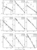 |
Fig. B.1 Radio SEDs of 31 IFRS in CDFS and ELAIS-S1 not shown in Fig. 2, using all available flux density data points and upper limits. The solid line shows the fit which was found to best describe the photometric detections as discussed in Sect. 3. Spectral index and – if applicable – turnover frequency of the best fit are quoted. We also show the first approach to describe the data – a single power law fitted to all photometric detections – by a dotted line if this fit was discarded later in the analysis. 1σ uncertainties of the single power law fits are represented by the shaded areas. Error bars show 1σ uncertainties. The frequency coverage varies from one IFRS to another and the flux density scales are different. |
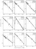 |
Fig. B.1 continued. |
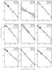 |
Fig. B.1 continued. |
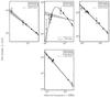 |
Fig. B.1 continued. |
All Tables
Characteristics of the observations of the ELAIS-S1 field, covering 15 IFRS from our sample.
Characteristics of the observations of the CDFS field, covering 19 IFRS from our sample.
All Figures
|
Fig. 1 Plateau de Bure Interferometer map (greyscale) of IFRS xFLS 478 at 105 GHz (2.9 mm) overlaid with the VLA 1.4 GHz radio contours from Condon et al. (2003), starting at 3σ and increasing by factors of 4. |
| In the text | |
|
Fig. 2 Radio SEDs of three IFRS in CDFS, using all available flux density data points and upper limits. The solid line shows the fit which was found to best describe the photometric detections as discussed in Sect. 3. Spectral index and – if applicable – turnover frequency of the best fit are quoted. We also show the first approach to describe the data – a single power law fitted to all photometric detections – by a dotted line if this fit was discarded later in the analysis. 1σ uncertainties of the single power law fits are represented by the shaded areas. Error bars show 1σ uncertainties. The frequency coverage varies from one IFRS to another and the flux density scales are different. The radio SEDs of the other 31 IFRS studied in this paper are shown in Fig. B.1. |
| In the text | |
|
Fig. 3 Histogram of the ATLAS DR3 spectral indices |
| In the text | |
|
Fig. 4 Radio spectral index α as a function of the 3.6 μm flux density (top left), α as a function of the radio flux density S1.4 GHz (top right), α as a function of the radio-to-IR flux density ratio S1.4 GHz/S3.6 μm (bottom left), and S1.4 GHz/S3.6 μm as a function of S1.4 GHz (bottom right) for our sample of 34 IFRS. The symbols distinguish subsamples of different turnover properties. Green dots represent sources with a detected turnover. Sources with a possible peak are shown by purple squares, and sources without a peak by black crosses. The classification is described in Sect. 3 and summarised for individual IFRS in Table 3. Upper and lower limits are represented by arrows. The grey horizontal and vertical lines indicate the medians or limits of the median. |
| In the text | |
|
Fig. 5 3.6 μm SWIRE map (Lonsdale et al. 2003; greyscale) of CS618 overplotted by the 1.4 GHz ATLAS DR3 (Franzen et al. 2015) contours. Contours start at 3σ and increase by factors of 4. CS618 is an evolved FRII radio galaxy with an unresolved core (centre of the shown map) and two slightly resolved lobes. |
| In the text | |
|
Fig. 6 Radio SED of IFRS xFLS 478. Error bars represent 1σ uncertainties. The black solid line shows the best fit of an SSA model. The fitted single power law is shown as black dotted line. The shaded area represents the 1σ uncertainty of the single power law fit. |
| In the text | |
|
Fig. 7 Modelling the radio-FIR SED of IFRS xFLS 478. The total SED (solid line) is composed of the SED of a star forming galaxy (dashed line) from Murphy (2009) and the radio SED of 00183 (dotted line) from Norris et al. (2012). The star forming SED template is again composed of synchrotron, free-free, and thermal dust components. The best model was found at z = 1.1 and is shown in this figure. Black dots represent the photometric data points of xFLS 478 with respective 1σ uncertainties. |
| In the text | |
|
Fig. B.1 Radio SEDs of 31 IFRS in CDFS and ELAIS-S1 not shown in Fig. 2, using all available flux density data points and upper limits. The solid line shows the fit which was found to best describe the photometric detections as discussed in Sect. 3. Spectral index and – if applicable – turnover frequency of the best fit are quoted. We also show the first approach to describe the data – a single power law fitted to all photometric detections – by a dotted line if this fit was discarded later in the analysis. 1σ uncertainties of the single power law fits are represented by the shaded areas. Error bars show 1σ uncertainties. The frequency coverage varies from one IFRS to another and the flux density scales are different. |
| In the text | |
|
Fig. B.1 continued. |
| In the text | |
|
Fig. B.1 continued. |
| In the text | |
|
Fig. B.1 continued. |
| In the text | |
Current usage metrics show cumulative count of Article Views (full-text article views including HTML views, PDF and ePub downloads, according to the available data) and Abstracts Views on Vision4Press platform.
Data correspond to usage on the plateform after 2015. The current usage metrics is available 48-96 hours after online publication and is updated daily on week days.
Initial download of the metrics may take a while.