| Issue |
A&A
Volume 592, August 2016
|
|
|---|---|---|
| Article Number | A138 | |
| Number of page(s) | 8 | |
| Section | The Sun | |
| DOI | https://doi.org/10.1051/0004-6361/201628851 | |
| Published online | 18 August 2016 | |
Flux rope proxies and fan-spine structures in active region NOAA 11897⋆
1 Key Laboratory of Solar Activity, National Astronomical Observatories, Chinese Academy of Sciences, 100012 Beijing, PR China
e-mail: This email address is being protected from spambots. You need JavaScript enabled to view it.
2 University of Chinese Academy of Sciences, 100049 Beijing, PR China
Received: 4 May 2016
Accepted: 28 June 2016
Abstract
Context. Flux ropes are composed of twisted magnetic fields and are closely connected with coronal mass ejections. The fan-spine magnetic topology is another type of complex magnetic fields. It has been reported by several authors, and is believed to be associated with null-point-type magnetic reconnection.
Aims. We try to determine the number of flux rope proxies and reveal fan-spine structures in the complex active region (AR) NOAA 11897.
Methods. Employing the high-resolution observations from the Solar Dynamics Observatory (SDO) and the Interface Region Imaging Spectrograph (IRIS), we statistically investigated flux rope proxies in NOAA AR 11897 from 14 November 2013 to 19 November 2013 and display two fan-spine structures in this AR.
Results. For the first time, we detect flux rope proxies of NOAA 11897 for a total of 30 times in four different locations during this AR’s transference from solar east to west on the disk. Moreover, we notice that these flux rope proxies were tracked by active or eruptive material of filaments 12 times, while for the remaining 18 times they appeared as brightenings in the corona. These flux rope proxies were either tracked in both lower and higher temperature wavelengths or only detected in hot channels. None of these flux rope proxies was observed to erupt; they faded away gradually. In addition to these flux rope proxies, we detect for the first time a secondary fan-spine structure. It was covered by dome-shaped magnetic fields that belong to a larger fan-spine topology.
Conclusions. These new observations imply that many flux ropes can exist in an AR and that the complexity of AR magnetic configurations is far beyond our imagination.
Key words: Sun: activity / Sun: atmosphere / Sun: coronal mass ejections (CMEs) / Sun: evolution / Sun: filaments, prominences / Sun: magnetic fields
Movies 1–8 are available in electronic form at http://www.aanda.org
© ESO, 2016
1. Introduction
A coronal mass ejection (CME) is a large-scale eruption from the solar atmosphere, releasing huge amounts of mass and magnetic flux into the interplanetary space. CMEs may severely affect the space environment at Earth (Gosling 1993; Webb et al. 1994). As shown in coronagraph images, a CME generally presents a three-part structure: a bright front or leading edge, an enclosed dark cavity, and an inner bright core (Illing & Hundhausen 1983; Chen 2011). The magnetic flux rope (MFR) is a set of magnetic field lines winding around a central axis, whose existence could explain the dark cavity’s accumulating magnetic energy and mass in a CME (Gibson et al. 2006; Riley et al. 2008; Wang & Stenborg 2010). The MFR has been thought to be closely connected with a CME, and almost all theoretical models of CMEs require the presence or formation of a coronal MFR (Forbes 2000). Thus, a complete research on the MFR is necessary to obtain a clear understanding of CMEs, which will undoubtedly result in accurate forecasts of CMEs and associated space weather.
An MFR can theoretically be formed in two ways: bodily flux emergence from below the photosphere into the upper atmosphere, or magnetic reconnection of sheared arcades in the corona. In the emergence model, a twisted MFR is assumed to exist below the photosphere and then to emerge into a pre-existing coronal potential field (Fan 2001, 2010; Manchester et al. 2004; Magara 2006). Okamoto et al. (2008) found that two opposite-polarity regions connected by a vertically weak but horizontally strong magnetic field first grew laterally and then narrowed. The horizontal magnetic field changed its orientation, which was accompanied by a significant blueshift. As a result, the authors suggested that an MFR emerging from below the photosphere had been observed. Vargas Domínguez et al. (2012) interpreted the same observation as a result of photospheric magnetic cancellation instead of flux emergence. In the reconnection model, magnetic reconnection between two bundles of opposite J-shaped loops, which have frequently been observed as the sigmoidal structure in the extreme ultraviolet (EUV) and X-ray lines, is able to form the MFR (Canfield et al. 1999; McKenzie & Canfield 2008; Liu et al. 2010; Green et al. 2011). A related possible original mechanism is that the MFR is built up and heated by the magnetic reconnection in the quasi-separatrix layers (Guo et al. 2013).
Considerable efforts have also been made in numerical simulations to study the formation and dynamic behavior of MFRs (Forbes & Priest 1995; Lin et al. 1998; Aulanier et al. 2010). Amari et al. (2000, 2003) simulated the evolution of an MFR and found that a slowly converging motion of the field lines’ footpoints toward the polarity inversion line helps to produce an MFR through magnetic reconnection. Török & Kliem (2003, 2005) studied the instability of an MFR and found that the kink and/or torus instability of the MFR can trigger a CME. Olmedo & Zhang (2010) made a more detailed study and proposed that the eruption of the MFR can be fully driven by a partial torus instability. Furthermore, setting the observed photospheric vector magnetic field as the bottom boundary, nonlinear force-free field extrapolation method was applied to reconstruct the topology of the MFR in the corona (Canou et al. 2009; Guo et al. 2010; Jiang et al. 2013).
Direct observations of MFRs have been reported with the help of multiwavelength observations from the Atmospheric Imaging Assembly (AIA; Lemen et al. 2012) onboard the Solar Dynamics Observatory (SDO; Pesnell et al. 2012). MFRs are typically detected in higher temperature passbands, such as 94 Å and 131 Å (Zhang et al. 2012; Cheng et al. 2013). Furthermore, MFRs sometimes appear one by one in the same region with a similar morphology, which are called homologous flux ropes (Li & Zhang 2013b). Li & Zhang (2013a) and Yang et al. (2014) reported that the fine-scale structures of MFRs can be tracked by erupting material once in a while and could be observed in both higher and lower temperature channels.
Despite a large amount of research on flux ropes, statistical investigations are rare. Recently, Zhang et al. (2015) have counted the number of the flux rope proxies over the visible solar disk from 2013 January to 2013 December and pointed out that in some particularly active regions, many flux rope proxies were detected, which showed some clustering. Our study mainly concerns flux rope proxies in NOAA 11897 and determines the locations and number of flux rope proxies during the AR’s evolution from 14 November 2013 to 19 November 2013. When we observe a set of EUV loops which collectively wind around a central and axial line, we consider them as a flux rope proxy. In addition to the statistical results, four examples of these flux rope proxies and two fan-spine structures are displayed. Fan-spine magnetic topology is another type of complex fields and has been proposed by several authors (Wang & Liu 2012; Sun et al. 2013). The fan-spine magnetic topology is believed to play a crucial role in solar explosive events, and direct observations of such a structure have been rare.
The remainder of this paper is structured as follows. Section 2 contains the observations and data analysis used for our study. The distribution of the flux rope proxies in NOAA 11897, four typical cases, and two fan-spine structures are presented in Sect. 3. Finally, we conclude this work and discuss the results in Sect. 4.
2. Observations and data analysis
The AIA onboard SDO observes the multilayered solar atmosphere, including the photosphere, chromosphere, transition region, and corona, in ten (E)UV passbands with a cadence of 12 s and a spatial sampling of 0.′′6 pixel-1, among which the 131 Å channel shows the flux rope best. We therefore focus on 131 Å in this study, while the 171 Å and 304 Å channel observations are also presented. To study the relationship between the photospheric magnetic fields of the AR and the flux rope proxy locations, line-of-sight (LOS) magnetograms from the SDO/Helioseismic and Magnetic Imager (HMI; Schou et al. 2012) with a time cadence of 45 s and a pixel size of 0.′′5 are used as well. Since it is difficult to exclude the possibility that some polarity was produced by the projection effect when NOAA AR 11897 was located close to the solar limb, we adopted the observations from 14 to 19 November 2013, when this AR was located at a distance away from the limbs.
Moreover, two series of the Interface Region Imaging Spectrograph (IRIS; De Pontieu et al. 2014) slit-jaw 1400 Å images (SJIs) are adopted as well, which are all Level 2 data. The 1400 Å channel contains emission from the Si IV 1394/1403 Å lines that are formed in the lower transition region. On 14 November 2013, the SJIs in 1400 Å focused on NOAA 11897 were taken from 20:09 UT to 20:35 UT with a pixel scale of 0.′′166, a cadence of 10 s, and a field of view (FOV) of 119′′× 119′′. On 17 November, the 1400 Å SJIs focused on the same AR were obtained from 12:58 UT to 13:47 UT with a FOV of 167′′× 174′′, and the same cadence and pixel size as on 14 November.
3. Results
3.1. Overview of the observed flux rope proxies
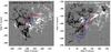 |
Fig. 1 SDO/HMI LOS magnetograms showing the magnetic fields of NOAA AR 11897. Red and blue solid curves outline the four locations of detected flux rope proxies in the AR from 14 to 19 November 2013. The red curves mean that the flux rope proxies on these locations can be detected only in hot EUV passbands, for example, 131 Å, while the blue curves mean that the proxies on these locations can be detected both in hot and cooler EUV passbands, such as 131 Å, 171 Å, and 304 Å. The temporal evolution of the LOS magnetograms is available as a movie (1.mp4) online. |
Distribution of the detected flux rope proxies.
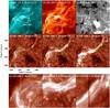 |
Fig. 2 Panels a)–c): SDO AIA 131 Å and 304 Å images and HMI LOS magnetogram displaying a flux rope proxy on 14 November 2013 in different temperature lines and its underlying magnetic field. Panels d)–f): IRIS 1400 Å images showing the brightening of this flux rope proxy. Panels g)–i): three extended 1400 Å images outlined by corresponding green squares in panels d)–f). The blue curves delineate the twisted threads of the flux rope proxy. The full temporal evolution of the 1400 Å, 131 Å, and 304 Å images is available as a movie (2.mp4) online. |
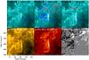 |
Fig. 3 Panels a)–c): sequence of AIA 131 Å images showing a flux rope proxy tracked by active material of a filament on 17 November 2013. The blue and red curves in panel b) are contours of corresponding negative and positive magnetic fields, respectively. Panels d)–f): corresponding 171 Å and 304 Å images and HMI LOS magnetogram. In panel f), the black square denotes the positive-polarity field region where this flux rope proxy’s northwest end is rooted, while the white square denotes the negative-polarity field region at the other end. These two squares are also shown in panel c). The blue dashed line represents the main axis of this flux rope proxy. An animation (3.mp4) of the 131 Å, 171 Å, and 304 Å images is available online. |
During the evolution of NOAA 11897 from 14 to 19 November 2013, we identify flux rope proxies for 30 times in four different locations by using coordinated observations from the SDO and the IRIS. The locations and general morphologies of these proxies are shown in Fig. 1 and the daily distribution is summarized in Table 1. The morphologies of some proxies in one location may change slowly with the evolution of the underlying magnetic field (see movie 1), but we classified these flux rope proxies into the same location by tracing their footpoints’ motion. According to our observations, some flux rope proxies can be detected in all seven EUV channels (304 Å, 171 Å, 193 Å, 211 Å, 335 Å, 94 Å, and 131 Å) that cover the temperatures from 0.05 MK to 20 MK while the others could only be observed in hot channels such as 94 Å and 131 Å. As a result, we roughly classify these proxies into two types. To distinguish them, we take the blue and red solid curves to outline these two types of flux rope proxy locations in Fig. 1. In the following part, we choose four typical samples to investigate these flux rope proxies in detail. The first two proxies can be observed in both lower and higher temperature lines, and the latter two can be only detected in higher temperature lines.
3.2. Two flux rope proxies detected in both lower and higher temperature wavelengths
A flux rope proxy on 14 November 2013 in L1 of Fig. 1a was selected and is shown in Fig. 2, which was associated with a filament activation (see movie 2). This filament was located along the neutral line of NOAA 11897 (see panel (c)), and the rope proxy was brightened by the filament active material in both lower and higher temperature channels around 20:13 UT (panels (a)–(b)). In the IRIS 1400 Å channel, we can clearly observe the brightening of this rope proxy (panels (d)–(f)). At 20:10 UT, the emission at the southeast end of this rope proxy was enhanced, which may result from the underneath magnetic flux cancellation (see panel (c)). Twisted structures were observed as a result of this brightening (see panel (g)). Then the brightening propagated to the north end and traced the whole flux rope proxy at 20:15 UT (see panels (e)–(f)). Some local twisted structures are shown in panels (h)–(i). By examining the fine-scale twisted structures in this flux rope proxy, we roughly estimate that the twist number of this proxy is about 4 π. From 20:15 UT to 20:18 UT, a rotation motion of the rope was observed (see movie 2), which can be identified as the unwinding motion of the twisted magnetic field lines (Yan et al. 2014). Meanwhile, the brightening material moved bidirectionally along the rope proxy. Later, a rotation motion was detected once again around the southeast end of this rope proxy from 20:20 UT to 20:23 UT.
Another flux rope proxy that was observed in the lower and higher temperature wavelengths was located at another polarity inversion line of NOAA 11897 (see L3 in Fig. 1b) on 17 November 2013 (see movie 3). Similar to the first flux rope proxy, the rope proxy shown in Fig. 3 was related to a filament as well. Around 10:16 UT, the filament was initially disturbed and accompanied by EUV brightening (panel (a)). Then the brightening material moved bidirectionally along the neutral line (panel (b)), and ten minutes later, a sigmoid flux rope proxy appeared in the lower and higher temperature wavelengths (see panels (c)−(e)). Twisted structures (see arrows in panels (a)−(c)) were tracked by the brightening material in the lower and higher temperature channels. The twist number of this proxy is estimated as 2 π. At 10:22 UT, this rope proxy was entirely traced out and the EUV emission of its southeast end increased after the arrival of brightening material. After this, the rope proxy’s spatial scale decreased gradually as well as the EUV intensity, until the proxy completely vanished at 10:38 UT. Nearly the whole of this rope proxy was similar in different channels except that the north part of the proxy could only be detected in hot channel (see panels (c)−(e)). Checking the HMI LOS magnetogram, we find that the northwest end of the flux rope proxy was rooted in the positive fields and the southeast end in negative fields (see panel (f)).
3.3. Two flux rope proxies detected only in the higher temperature wavelengths
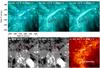 |
Fig. 4 Panels a)−c): AIA 131 Å images exhibiting a flux rope proxy on 14 November 2013. The blue square in panel a) outlines the FOV of panels d) and e). Panels d)−e): corresponding HMI LOS magnetograms showing the evolution of the underneath magnetic fields. The red squares denote the region where magnetic cancellation occurred. Panel f): AIA 304 Å image with the same FOV of panels a)−c) displaying this rope proxy in a lower temperature channel. The temporal evolution of the 131 Å and 304 Å images is available as a movie (4.mp4) online. |
Except for the flux rope proxies detected in both lower and higher temperature channels, other rope proxies could only be detected in hot lines. The first case took place on 14 November 2013 in L2 of Fig. 1a and is shown in Fig. 4. In this case, the flux rope proxy was initiated by a partial eruption of a filament (see movie 4) and the flux cancellation underlying this proxy was observed as well (panels (d) and (e)). At 10:55 UT, brightening filament material appeared in the 304 Å and 131 Å channels (panel (a)). But during the following ten minutes, the brightening material moved along the two directions of the filament channel, tracking the rope proxy (panel (b)) only in the 131 Å passband. The twisted structures (see arrows in panels (b)−(c)) were tracked by the brightening material in the hot channel as well. Here we estimate that this proxy’s twist number is about 2 π. The rope proxy was well developed at 11:06 UT (panel (c)) and faded away about 20 min later. In the lower temperature line (e.g., 304 Å), we were unable to observe the main body of this rope proxy except for the brightening footpoints (see arrow in panel (f)).
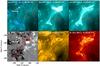 |
Fig. 5 Panels a)−c): sequence of AIA 131 Å images displaying a flux rope proxy tracked by a filament’s active material on 15 November 2013. The blue and red curves in panel a) are contours of corresponding negative and positive magnetic fields, respectively. Panels d)−f): corresponding HMI LOS magnetogram, AIA 171 Å and AIA 304 Å images. In panel d), the black curve outlines the general shape of the filament, and the red curve is the contour of brightness in panel c). An animation (5.mp4) of the 131 Å, 171 Å, and 304 Å channels shown in this figure is available in the online. |
Another flux rope proxy of this type was observed on 15 November 2013 in L4 of Fig. 1b (see movie 5). This rope proxy was initiated by a failed eruption of a filament (see Fig. 5a). In the 131 Å channel, the filament material began to brighten at 11:32 UT. Then the brightening material moved to the southeast and tracked the rope proxy during the following ten minutes (panel (b)), which was accompanied by a C7.6 flare. The arrows in panels (b)−(c) point out the twist of this proxy, and we estimate that the twist number is about π. At 11:42 UT, the rope proxy was well developed (panel (c)). Then the brightening material moved back to the filament again, and the rope proxy faded away ten minutes later. We outline the general shapes of the proxy and the filament in panel (d), which show the filament’s position relative to the proxy. Similar to the example shown in Fig. 4, this rope proxy’s main body cannot be detected in the lower temperature wavelengths, such as 171 Å and 304 Å (see panels (e) and (f)).
3.4. Two fan-spine structures
In NOAA 11897, we also detected two fan-spine structures in addition to the flux rope proxies shown above. The first structure was observed on 18 November 2013 (see movie 6). At 04:10 UT, a quasi-circular ribbon, whose radius was about 20 Mm, began to brighten in the 131 Å, 171 Å, and 304 Å channels. Subsequently, the bright thread-like structures in the 131 Å wavelength appeared and composed a twisted loop bundle with its eastern end connecting to the circular ribbon, while the other end was connected to the remote brightening region (see Figs. 6a−c). Thus a dome-shaped structure formed and covered the quasi-circular ribbon. Then the dome and the loop bundle composed an obvious fan-spine configuration. This event was accompanied by a C2.8 flare. However, the fan-spine configuration could not be observed in the lower temperature lines, such as 171 Å and 304 Å (see panels (d) and (e)). As a result, we suggest that plasma filled in the fan-spine structure is very hot and exactly above 10 MK (Sun et al. 2013). The circular ribbon corresponded to the intersection of a fan surface with the photosphere, and it was observed in both lower and higher temperature wavelengths during the whole period. Moreover, an apparent slipping motion of the fine structure along the circular ribbon and the shuffling motion within the hot loop bundle were clearly observed. At about 04:40 UT, the bright ribbon faded away and the fan-spine configuration disappeared later at 04:50 UT. From examining the evolution of the underneath magnetic fields (see movie 1), we note that a new dipole emerged around 04:30 UT on 16 November (see the orange region in panel (g)) at the location of the circular ribbon, which was about two days before the fan-spine structure appeared (see the green region in panel (g)). Then the negative polarity of this new dipole was integrated into pre-existing ambient negative fields on the east side, while the positive part continued to grow, which was surrounded by the negative fields in the end. Rapid magnetic flux cancellation occurred successively between the new positive field and the surrounding negative fields. During the cancellation process, the fan-spine structure brightened again at about 16:00 UT (see the blue region in panel (g)), and a C2.6 flare was detected simultaneously. By comparing the AIA 131 Å image and HMI LOS magnetogram, we found that the quasi-circular ribbon lay on the surrounding negative fields and the fan-spine structure connected this ribbon to remote positive fields (see panels (c) and (f)).
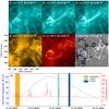 |
Fig. 6 Panels a)−c): AIA 131 Å images displaying a fan-spine structure on 18 November 2013. Panels d)−f): corresponding AIA 171 Å and 304 Å images and HMI LOS magnetogram. In panel f), the black squares denote the positive magnetic field regions where this flux rope proxy’s northwest ends are rooted, while the white square denotes the negative field region at the other end and they are also shown in panel c). Panel g): total positive magnetic flux (blue curve) and brightness (red curve) of the region shown by the white square in panel f) from 16 November 00:00 UT to 20 November 00:00 UT. The orange region marks the start of the magnetic field’s emergence, while the green and blue regions denote the brightening events of the structure. An animation (6.mp4) of the 131 Å, 171 Å, and 304 Å images is available online. |
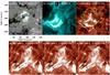 |
Fig. 7 Panels a)−c): HMI LOS magnetogram, AIA 131 Å image, and SJI of 1400 Å showing the first fan-spine structure earlier on 17 November 2013. The yellow dashed circles in panels a) and c) delineate the bright ribbon while the blue dashed circles denote the secondary fan-spine structure covered by the dome displayed in Fig. 6. The green squares outline the FOV of panels d)−f). Panels d)−f): extended SJIs of 1400 Å exhibiting the secondary fan-spine structure. The black triangles track the material’s flowing toward the southeast. The full temporal evolution of the 1400 Å and 131 Å images is available as a movie (7.mp4) online. |
To study the fine structures of this fan-spine structure, we employed the IRIS 1400 Å data and compared them with the corresponding SDO HMI LOS magnetogram and AIA 131 Å image (see Fig. 7). Although the 1400 Å observations only covered the period from 12:58 UT to 13:47 UT on 17 November, they first revealed a secondary fan-spine structure (see movie 7). The quasi-circular ribbon was clear in the 1400 Å channel, and we noted that it was rooted in the surrounding negative fields (see the yellow dashed lines in panels (a) and (c)). Inside this ribbon, we detected a smaller quasi-circular ribbon with a radius of about 6.4 Mm, which lay on the inner ring of positive magnetic fields with negative fields inside (see the blue dashed lines in panels (a) and (c)). Moreover, a secondary fan-spine configuration above this smaller circular ribbon was observed in the 131 Å and 1400 Å wavelengths (see the green squares in panels (a)−(c)). In panels (d)−(f), 1400 Å images are zoomed to show the secondary fan-spine configuration. Similar to the structure shown in Fig. 6, this fan-spine structure connected the smaller quasi-circular brightening ribbon to remote negative fields near the outer ribbon, which formed a nested dome shape. During the evolution of this fan-spine structure, a bidirectional flow was observed as well. The flow toward the southeast is marked by tracing brightening plasmoids, whose projected velocities were around 114 km s-1 (see the black triangles in panels (d)−(f)).
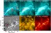 |
Fig. 8 Panels a)−c): AIA 131 Å images showing another fan-spine structure on 16 November 2013. The blue dashed circles outline the quasi-circular ribbon. The blue and red curves in panel a) are contours of corresponding negative and positive magnetic fields, respectively. Panels d)−f): corresponding HMI LOS magnetogram, AIA 171 Å and AIA 304 Å images. The red curve in panel e) is the contour of the remote brightening ribbon and is also shown in panels b) and d). An animation (8.mp4) of the 131 Å, 171 Å, and 304 Å channels shown in this figure is available in the online. |
The second fan-spine structure was observed on 16 November 2013 (see movie 8). At about 07:57 UT, a set of loops began to brighten in the 131 Å passband, which connected a quasi-circular ribbon to a remote brightening ribbon (see Fig. 8a). Then the fan-spine structure was traced out clearly. Moreover, a sequential brightening of the circular ribbon and an apparent shuffling motion within the hot loop bundle were detected, which have also been noted in the first case. But in the lower temperature channels, we were only able to see the quasi-circular ribbon and remote brightening ribbon (see panels (e) and (f)). At 08:15 UT, the fan-spine structure was well developed (see panel (b)). After this, the emission of the loops in the 131 Å channel began to weaken. But at about 08:35 UT, the brightening loops appeared in the 171 Å and 304 Å channels. We suggest that the brightening loops appearing in 171 Å and 304 Å channels were previous loops in the 131 Å channel that had undergone a cooling process. Near 09:35 UT, this fan-spine structure disappeared. Investigating the evolution of the underlying magnetic fields (see movie 1), we find that negative fields emerged near the location of the quasi-circular ribbon, which was surrounded by positive fields, at about 22:00 UT on 14 November. It is similar to the case on 18 November, where the opposite field emergence occurred several days earlier than the fan-spine structure appeared at the location of the quasi-circular ribbon. Moreover, the quasi-circular ribbon lay on the surrounding positive fields and the fan-spine structure connected the ribbon to remote negative fields (see panel (d)).
4. Conclusions and discussion
Employing high-resolution observations from the SDO and the IRIS, we statistically investigated flux rope proxies in the NOAA 11897 from 14 November 2013 to 19 November 2013. For the first time, we detected flux rope proxies for 30 times in NOAA 11897 in four different locations during six days, that is, five times per day on average. In this work, we illuminated that flux rope proxies can appear frequently and be distributed in different locations in an AR. Lites (2005) speculated that flux ropes might be rather common in normal active regions, which is verified by our observations here. In particular, we showed two flux rope proxies tracked in both lower and higher temperature wavelengths and two brightening rope proxies detected only in hot channels. To better assess these four flux rope proxies, we roughly estimated their twist numbers. By examining the fine-scale twisted structures of the flux rope proxy in Fig. 2, we estimate that the twist number of this proxy is about 4 π, that is, 2 π is detected in Fig. 2g, π in Fig. 2h, and π in Fig. 2i. As some twisted structures of this proxy cannot be detected, the twist number 4 π may be considered as a lower limit. In the late stage of this proxy’s evolution, two rotation motions were detected successively. Because the minimum twist number (4 π) of this proxy is above the critical value (2.5 π~ 3.5 π; Hood & Priest 1981), we suggest that kink instability might have occurred in this event, and the rotation was obviously the unwinding motion of the twisted magnetic field lines. As a result, the flux rope proxy disappeared in this location (L1) after the rotation motions. For the flux rope proxies in Figs. 3–5, no rotation motions took place and their twist numbers had no great changes. We therefore estimated an average lower limit of the twist number for each proxy, which is 2 π, 2 π, and π. Some authors considered a full turn to be the qualifying property (e.g., Liu et al. 2016), but others considered a half turn to be sufficient (e.g., Chintzoglou et al. 2015). Our results in this work are consistent with the study of Chintzoglou et al. (2015), who considered a half turn (π) to be sufficient for judging a flux rope, as all the four flux rope proxies satisfy such a standard. In addition to these flux rope proxies, we reported on two fan-spine structures in detail.
It is worth mentioning that these four locations were not invariant all the time, but moved or were slowly deformed with the evolution of the underlying magnetic fields. Tracing the ends of two flux rope proxies through HMI LOS magnetograms, we decided to classify them into the same location when these two ropes’ both ends were in the same regions, otherwise we determined them as two different locations. Furthermore, in two locations (L2 and L4 in Fig. 1) of the four, flux rope proxies could only be detected in higher temperature wavelengths (Cheng et al. 2011; Zhang et al. 2012), while the flux rope proxies in the other two locations (L1 and L3 in Fig. 1) have both lower and higher temperature components (Li & Zhang 2013c). In NOAA 11897, the flux rope proxies that can be seen in both cool and hot lines (L1 and L3) follow the polarity neutral line much more closely than the proxies that appear only in hot lines (L2 and L4). We suggest that in L2 and L4, these flux rope proxies detected only in hot lines may be purely coronal arches at a great height. As for L1 and L3, the proxies that could be detected in both cool and hot channels may exist at low heights within filament channels. We suggest that near the polarity neutral line, cool materials of filaments tend to converge within the flux rope structure. Meanwhile, interaction of the opposite polarity fields around the polarity neutral line may heat up local filament material. As a result, flux rope proxies near the polarity neutral line (L1 and L3) own complicated temperature features.
Here we note that flux rope proxies appeared in one location several times. It is possible that seven flux ropes were detected in four different locations and were repeatedly illuminated for 30 times in total. Since the flux rope proxies in L3 (L4) lasted four days and showed a very different complexity in their geometry when they reappeared, we suggest that there were three (two) flux rope proxies in L3 (L4). In L3, we consider the proxy detected twice on 16 November as the first in this location, the proxy detected six times on 17 and 18 November as the second, and the proxy detected once on 19 November as the third. Moreover, in L4, the proxy detected seven times on 15 and 16 November is identified as the first in this location, and the proxy detected twice on 17 and 18 November is identified as the second. For L1 and L2, probably only one flux rope proxy in each of these locations was detected and repeatedly illuminated. The flux rope proxies that appeared in one location for several times may also be described as homologous flux ropes according to Li & Zhang (2013b). These authors defined the homologous flux ropes as follows: (1) originating from the same region within the same AR; (2) whose endpoints are anchored at the same location; (3) whose morphologies resemble each other. Synthesizing Table 1 and Fig. 1, we can clearly find that flux rope proxies appeared with remarkable frequency in L2, L3, and L4. During the evolution of this AR’s magnetic field (see movie attached to Fig. 1), the positive-polarity field underlying the L2 northwestern ends slowly moved north-westward along the neutral line, while the negative field underlying the southeastern ends was generally still. Thus we consider that the frequent appearance of flux rope proxies in L2 may result from the underlying magnetic field’s lasting shear motion (Amari et al. 1999, 2000). As for L3, Fig. 1b clearly shows that it was located above the main polarity neutral line of NOAA 11897. Considering the long-term existence of this main neutral line, it is explicable that flux rope proxies were observed nine times in L3 from 16 to 19 November. In L4, flux rope proxies were detected nine times from 15 to 18 November, which may result from the underlying strong magnetic fields. Flux rope proxies in this location connected a pair of strong magnetic fields, which existed throughout the entire observation period. Moreover, this pair of strong magnetic fields continuously canceled out with the surrounding opposite-polarity magnetic fields, and flux cancellation is thought to be the primary formation mechanism of flux ropes (Savcheva et al. 2012a,b). We followed the evolution of the AR and found that three pairs of magnetic fields emerged. Flux rope proxies were detected for 27 times in the emerging and stable phase of the magnetic flux. In the decaying phase, only 10% flux rope proxies (three times) were detected, implying an unbalanced distribution of the flux ropes during the entire AR evolution. We note that none of these flux ropes has been observed to erupt in the end, and all of them just faded away gradually.
An in-depth research on the fan-spine configuration has been proposed by several authors (Wang & Liu 2012; Sun et al. 2013). In the work of Sun et al. (2013), flux emergence was believed to result in a largely closed fan-spine topology. The sequential brightening of the circular ribbon and the apparent shuffling motion within the hot loop bundle indicated the slipping-type reconnection (Li & Zhang 2015). Here we reported two examples that have a conspicuous fan-spine configuration, apparent sequential brightening along the circular ribbon, and shuffling motion within the loop bundle in the 131 Å passband. New flux emergence took place several days prior to the fan-spine structure’s appearance in both cases. Priest & Démoulin (1995) showed that reconnections may also occur in quasi-separatrix layers (QSLs) where magnetic connectivity is continuous but with steep gradient. Field lines may continuously slip within QSLs to exchange their footpoints, which is an extension of the instantaneous break-and-paste scenario (Aulanier et al. 2006, 2007). The fan-spine topology (Lau & Finn 1990) often arises with new flux emergence into a pre-existing field. Part of the new field becomes parasitic and surrounded by the opposite fields. Then a null point forms in the corona (Török et al. 2009). Energized particles from reconnection near the null point flow along the QSLs, brightening their footpoints, which is the quasi-circular ribbons in our work. For the first time, we detected a secondary fan-spine structure on 17 November 2013. In the spine, the bidirectional flow was observed, and we suggest that the flow may be caused by the null-point-type reconnection as well. Moreover, we noted EUV irradiance delays in lower temperature channels. The brightening loops connecting the quasi-circular ribbon to the remote brightening ribbon were formed in the fan-spine structure and were heated to over 10 MK (Sun et al. 2013). The delay of the brightening loops’ appearance in cooler channels, such as 171 Å and 304 Å, suggests a cooling process (Liu et al. 2013).
Online material
Movie of Fig. 1 Access Supplementary Material
Movie of Fig. 2 Access Supplementary Material
Movie of Fig. 3 Access Supplementary Material
Movie of Fig. 4 Access Supplementary Material
Movie of Fig. 5 Access Supplementary Material
Movie of Fig. 6 Access Supplementary Material
Movie of Fig. 7 Access Supplementary Material
Movie of Fig. 8 Access Supplementary Material
Acknowledgments
We thank the referee for the valuable suggestions. The data are used courtesy of the SDO and IRIS science teams. SDO is a mission of NASA’s Living With a Star Program. IRIS is a NASA small explorer mission developed and operated by LMSAL with mission operations executed at NASA Ames Research center and major contributions to downlink communications funded by ESA and the Norwegian Space Centre. This work is supported by the National Natural Science Foundations of China (11533008 and 11303050) and the Strategic Priority Research Program − The Emergence of Cosmological Structures of the Chinese Academy of Sciences (Grant No. XDB09000000).
References
- Amari, T., Luciani, J. F., Mikic, Z., & Linker, J. 1999, ApJ, 518, L57 [NASA ADS] [CrossRef] [Google Scholar]
- Amari, T., Luciani, J. F., Mikic, Z., & Linker, J. 2000, ApJ, 529, L49 [NASA ADS] [CrossRef] [PubMed] [Google Scholar]
- Amari, T., Luciani, J. F., Aly, J. J., Mikic, Z., & Linker, J. 2003, ApJ, 585, 1073 [NASA ADS] [CrossRef] [Google Scholar]
- Aulanier, G., Pariat, E., Démoulin, P., & DeVore, C. R. 2006, Sol. Phys., 238, 347 [NASA ADS] [CrossRef] [Google Scholar]
- Aulanier, G., Golub, L., DeLuca, E. E., et al. 2007, Science, 318, 1588 [NASA ADS] [CrossRef] [Google Scholar]
- Aulanier, G., Török, T., Démoulin, P., & DeLuca, E. E. 2010, ApJ, 708, 314 [Google Scholar]
- Canfield, R. C., Hudson, H. S., & McKenzie, D. E. 1999, Geophys. Res. Lett., 26, 627 [Google Scholar]
- Canou, A., Amari, T., Bommier, V., et al. 2009, ApJ, 693, L27 [NASA ADS] [CrossRef] [Google Scholar]
- Chen, P. F. 2011, Liv. Rev. Sol. Phys., 8, 1 [Google Scholar]
- Cheng, X., Zhang, J., Liu, Y., & Ding, M. D. 2011, ApJ, 732, L25 [NASA ADS] [CrossRef] [Google Scholar]
- Cheng, X., Zhang, J., Ding, M. D., Liu, Y., & Poomvises, W. 2013, ApJ, 763, 43 [NASA ADS] [CrossRef] [Google Scholar]
- Chintzoglou, G., Patsourakos, S., & Vourlidas, A. 2015, ApJ, 809, 34 [NASA ADS] [CrossRef] [Google Scholar]
- De Pontieu, B., Title, A. M., Lemen, J. R., et al. 2014, Sol. Phys., 289, 2733 [NASA ADS] [CrossRef] [Google Scholar]
- Fan, Y. 2001, ApJ, 554, L111 [NASA ADS] [CrossRef] [Google Scholar]
- Fan, Y. 2010, ApJ, 719, 728 [NASA ADS] [CrossRef] [Google Scholar]
- Forbes, T. G. 2000, J. Geophys. Res., 105, 23153 [NASA ADS] [CrossRef] [Google Scholar]
- Forbes, T. G., & Priest, E. R. 1995, ApJ, 446, 377 [NASA ADS] [CrossRef] [Google Scholar]
- Gibson, S. E., Foster, D., Burkepile, J., de Toma, G., & Stanger, A. 2006, ApJ, 641, 590 [NASA ADS] [CrossRef] [Google Scholar]
- Gosling, J. T. 1993, J. Geophys. Res., 98, 18937 [NASA ADS] [CrossRef] [Google Scholar]
- Green, L. M., Kliem, B., & Wallace, A. J. 2011, A&A, 526, A2 [NASA ADS] [CrossRef] [EDP Sciences] [Google Scholar]
- Guo, Y., Schmieder, B., Démoulin, P., et al. 2010, ApJ, 714, 343 [NASA ADS] [CrossRef] [Google Scholar]
- Guo, Y., Ding, M. D., Cheng, X., Zhao, J., & Pariat, E. 2013, ApJ, 779, 157 [NASA ADS] [CrossRef] [Google Scholar]
- Hood, A. W., & Priest, E. R. 1981, Geophys. Astrophys. Fluid Dyn., 17, 297 [NASA ADS] [CrossRef] [Google Scholar]
- Jiang, C., Feng, X., Wu, S. T., & Hu, Q. 2013, ApJ, 771, L30 [NASA ADS] [CrossRef] [Google Scholar]
- Illing, R. M. E., & Hundhausen, A. J. 1983, J. Geophys. Res., 88, 10210 [NASA ADS] [CrossRef] [Google Scholar]
- Lau, Y.-T., & Finn, J. M. 1990, ApJ, 350, 672 [NASA ADS] [CrossRef] [Google Scholar]
- Lemen, J. R., Title, A. M., Akin, D. J., et al. 2012, Sol. Phys., 275, 17 [NASA ADS] [CrossRef] [Google Scholar]
- Li, T., & Zhang, J. 2013a, ApJ, 770, L25 [NASA ADS] [CrossRef] [Google Scholar]
- Li, T., & Zhang, J. 2013b, ApJ, 778, L29 [NASA ADS] [CrossRef] [Google Scholar]
- Li, L. P., & Zhang, J. 2013c, A&A, 552, L11 [NASA ADS] [CrossRef] [EDP Sciences] [Google Scholar]
- Li, T., & Zhang, J. 2015, ApJ, 804, L8 [NASA ADS] [CrossRef] [Google Scholar]
- Lin, J., Forbes, T. G., Isenberg, P. A., & Demoulin, P. 1998, ApJ, 504, 1006 [NASA ADS] [CrossRef] [Google Scholar]
- Lites, B. W. 2005, ApJ, 622, 1275 [NASA ADS] [CrossRef] [Google Scholar]
- Liu, R., Liu, C., Wang, S., Deng, N., & Wang, H. 2010, ApJ, 725, L84 [NASA ADS] [CrossRef] [Google Scholar]
- Liu, K., Zhang, J., Wang, Y., & Cheng, X. 2013, ApJ, 768, 150 [NASA ADS] [CrossRef] [Google Scholar]
- Liu, R., Kliem, B., Titov, V. S., et al. 2016, ApJ, 818, 148 [NASA ADS] [CrossRef] [Google Scholar]
- Manchester, W., IV, Gombosi, T., DeZeeuw, D., & Fan, Y. 2004, ApJ, 610, 588 [NASA ADS] [CrossRef] [Google Scholar]
- Magara, T. 2006, ApJ, 653, 1499 [NASA ADS] [CrossRef] [Google Scholar]
- McKenzie, D. E., & Canfield, R. C. 2008, A&A, 481, L65 [NASA ADS] [CrossRef] [EDP Sciences] [Google Scholar]
- Okamoto, T. J., Tsuneta, S., Lites, B. W., et al. 2008, ApJ, 673, L215 [NASA ADS] [CrossRef] [Google Scholar]
- Olmedo, O., & Zhang, J. 2010, ApJ, 718, 433 [NASA ADS] [CrossRef] [Google Scholar]
- Pesnell, W. D., Thompson, B. J., & Chamberlin, P. C. 2012, Sol. Phys., 275, 3 [NASA ADS] [CrossRef] [Google Scholar]
- Priest, E. R., & Démoulin, P. 1995, J. Geophys. Res., 100, 23443 [NASA ADS] [CrossRef] [Google Scholar]
- Riley, P., Lionello, R., Mikić, Z., & Linker, J. 2008, ApJ, 672, 1221 [NASA ADS] [CrossRef] [Google Scholar]
- Savcheva, A., Pariat, E., van Ballegooijen, A., Aulanier, G., & DeLuca, E. 2012a, ApJ, 750, 15 [NASA ADS] [CrossRef] [Google Scholar]
- Savcheva, A. S., Green, L. M., van Ballegooijen, A. A., & DeLuca, E. E. 2012b, ApJ, 759, 105 [NASA ADS] [CrossRef] [Google Scholar]
- Schou, J., Scherrer, P. H., Bush, R. I., et al. 2012, Sol. Phys., 275, 229 [Google Scholar]
- Sun, X., Hoeksema, J. T., Liu, Y., et al. 2013, ApJ, 778, 139 [NASA ADS] [CrossRef] [Google Scholar]
- Török, T., & Kliem, B. 2003, A&A, 406, 1043 [NASA ADS] [CrossRef] [EDP Sciences] [Google Scholar]
- Török, T., & Kliem, B. 2005, ApJ, 630, L97 [Google Scholar]
- Török, T., Aulanier, G., Schmieder, B., Reeves, K. K., & Golub, L. 2009, ApJ, 704, 485 [NASA ADS] [CrossRef] [Google Scholar]
- Vargas Domínguez, S., MacTaggart, D., Green, L., van Driel-Gesztelyi, L., & Hood, A. W. 2012, Sol. Phys., 278, 33 [NASA ADS] [CrossRef] [Google Scholar]
- Wang, H., & Liu, C. 2012, ApJ, 760, 101 [NASA ADS] [CrossRef] [Google Scholar]
- Wang, Y.-M., & Stenborg, G. 2010, ApJ, 719, L181 [NASA ADS] [CrossRef] [Google Scholar]
- Webb, D. F., Forbes, T. G., Aurass, H., et al. 1994, Sol. Phys., 153, 73 [NASA ADS] [CrossRef] [Google Scholar]
- Yan, X. L., Xue, Z. K., Liu, J. H., Kong, D. F., & Xu, C. L. 2014, ApJ, 797, 52 [NASA ADS] [CrossRef] [Google Scholar]
- Yang, S., Zhang, J., Liu, Z., & Xiang, Y. 2014, ApJ, 784, L36 [NASA ADS] [CrossRef] [Google Scholar]
- Zhang, J., Cheng, X., & Ding, M.-D. 2012, Nature Communications, 3 [Google Scholar]
- Zhang, J., Yang, S. H., & Li, T. 2015, A&A, 580, A2 [NASA ADS] [CrossRef] [EDP Sciences] [Google Scholar]
All Tables
All Figures
|
Fig. 1 SDO/HMI LOS magnetograms showing the magnetic fields of NOAA AR 11897. Red and blue solid curves outline the four locations of detected flux rope proxies in the AR from 14 to 19 November 2013. The red curves mean that the flux rope proxies on these locations can be detected only in hot EUV passbands, for example, 131 Å, while the blue curves mean that the proxies on these locations can be detected both in hot and cooler EUV passbands, such as 131 Å, 171 Å, and 304 Å. The temporal evolution of the LOS magnetograms is available as a movie (1.mp4) online. |
| In the text | |
|
Fig. 2 Panels a)–c): SDO AIA 131 Å and 304 Å images and HMI LOS magnetogram displaying a flux rope proxy on 14 November 2013 in different temperature lines and its underlying magnetic field. Panels d)–f): IRIS 1400 Å images showing the brightening of this flux rope proxy. Panels g)–i): three extended 1400 Å images outlined by corresponding green squares in panels d)–f). The blue curves delineate the twisted threads of the flux rope proxy. The full temporal evolution of the 1400 Å, 131 Å, and 304 Å images is available as a movie (2.mp4) online. |
| In the text | |
|
Fig. 3 Panels a)–c): sequence of AIA 131 Å images showing a flux rope proxy tracked by active material of a filament on 17 November 2013. The blue and red curves in panel b) are contours of corresponding negative and positive magnetic fields, respectively. Panels d)–f): corresponding 171 Å and 304 Å images and HMI LOS magnetogram. In panel f), the black square denotes the positive-polarity field region where this flux rope proxy’s northwest end is rooted, while the white square denotes the negative-polarity field region at the other end. These two squares are also shown in panel c). The blue dashed line represents the main axis of this flux rope proxy. An animation (3.mp4) of the 131 Å, 171 Å, and 304 Å images is available online. |
| In the text | |
|
Fig. 4 Panels a)−c): AIA 131 Å images exhibiting a flux rope proxy on 14 November 2013. The blue square in panel a) outlines the FOV of panels d) and e). Panels d)−e): corresponding HMI LOS magnetograms showing the evolution of the underneath magnetic fields. The red squares denote the region where magnetic cancellation occurred. Panel f): AIA 304 Å image with the same FOV of panels a)−c) displaying this rope proxy in a lower temperature channel. The temporal evolution of the 131 Å and 304 Å images is available as a movie (4.mp4) online. |
| In the text | |
|
Fig. 5 Panels a)−c): sequence of AIA 131 Å images displaying a flux rope proxy tracked by a filament’s active material on 15 November 2013. The blue and red curves in panel a) are contours of corresponding negative and positive magnetic fields, respectively. Panels d)−f): corresponding HMI LOS magnetogram, AIA 171 Å and AIA 304 Å images. In panel d), the black curve outlines the general shape of the filament, and the red curve is the contour of brightness in panel c). An animation (5.mp4) of the 131 Å, 171 Å, and 304 Å channels shown in this figure is available in the online. |
| In the text | |
|
Fig. 6 Panels a)−c): AIA 131 Å images displaying a fan-spine structure on 18 November 2013. Panels d)−f): corresponding AIA 171 Å and 304 Å images and HMI LOS magnetogram. In panel f), the black squares denote the positive magnetic field regions where this flux rope proxy’s northwest ends are rooted, while the white square denotes the negative field region at the other end and they are also shown in panel c). Panel g): total positive magnetic flux (blue curve) and brightness (red curve) of the region shown by the white square in panel f) from 16 November 00:00 UT to 20 November 00:00 UT. The orange region marks the start of the magnetic field’s emergence, while the green and blue regions denote the brightening events of the structure. An animation (6.mp4) of the 131 Å, 171 Å, and 304 Å images is available online. |
| In the text | |
|
Fig. 7 Panels a)−c): HMI LOS magnetogram, AIA 131 Å image, and SJI of 1400 Å showing the first fan-spine structure earlier on 17 November 2013. The yellow dashed circles in panels a) and c) delineate the bright ribbon while the blue dashed circles denote the secondary fan-spine structure covered by the dome displayed in Fig. 6. The green squares outline the FOV of panels d)−f). Panels d)−f): extended SJIs of 1400 Å exhibiting the secondary fan-spine structure. The black triangles track the material’s flowing toward the southeast. The full temporal evolution of the 1400 Å and 131 Å images is available as a movie (7.mp4) online. |
| In the text | |
|
Fig. 8 Panels a)−c): AIA 131 Å images showing another fan-spine structure on 16 November 2013. The blue dashed circles outline the quasi-circular ribbon. The blue and red curves in panel a) are contours of corresponding negative and positive magnetic fields, respectively. Panels d)−f): corresponding HMI LOS magnetogram, AIA 171 Å and AIA 304 Å images. The red curve in panel e) is the contour of the remote brightening ribbon and is also shown in panels b) and d). An animation (8.mp4) of the 131 Å, 171 Å, and 304 Å channels shown in this figure is available in the online. |
| In the text | |
Current usage metrics show cumulative count of Article Views (full-text article views including HTML views, PDF and ePub downloads, according to the available data) and Abstracts Views on Vision4Press platform.
Data correspond to usage on the plateform after 2015. The current usage metrics is available 48-96 hours after online publication and is updated daily on week days.
Initial download of the metrics may take a while.