| Issue |
A&A
Volume 592, August 2016
|
|
|---|---|---|
| Article Number | A15 | |
| Number of page(s) | 12 | |
| Section | Stellar structure and evolution | |
| DOI | https://doi.org/10.1051/0004-6361/201628779 | |
| Published online | 04 July 2016 | |
The dependence of convective core overshooting on stellar mass
1 Instituto de Astrofísica de Andalucía, CSIC, Apartado 3004, 18080 Granada, Spain
e-mail: This email address is being protected from spambots. You need JavaScript enabled to view it.
2 Harvard-Smithsonian Center for Astrophysics, 60 Garden St., Cambridge, MA 02138, USA
Received: 22 April 2016
Accepted: 30 May 2016
Abstract
Context. Convective core overshooting extends the main-sequence lifetime of a star. Evolutionary tracks computed with overshooting are very different from those that use the classical Schwarzschild criterion, which leads to rather different predictions for the stellar properties. Attempts over the last two decades to calibrate the degree of overshooting with stellar mass using detached double-lined eclipsing binaries have been largely inconclusive, mainly because of a lack of suitable observational data.
Aims. We revisit the question of a possible mass dependence of overshooting with a more complete sample of binaries, and examine any additional relation there might be with evolutionary state or metal abundance Z.
Methods. We used a carefully selected sample of 33 double-lined eclipsing binaries strategically positioned in the H-R diagram with accurate absolute dimensions and component masses ranging from 1.2 to 4.4 M⊙. We compared their measured properties with stellar evolution calculations to infer semi-empirical values of the overshooting parameter αov for each star. Our models use the common prescription for the overshoot distance dov = αovHp, where Hp is the pressure scale height at the edge of the convective core as given by the Schwarzschild criterion, and αov is a free parameter.
Results. We find a relation between αov and mass, which is defined much more clearly than in previous work, and indicates a significant rise up to about 2 M⊙ followed by little or no change beyond this mass. No appreciable dependence is seen with evolutionary state at a given mass, or with metallicity at a given mass although the stars in our sample span a range of a factor of ten in [Fe/H], from −1.01 to + 0.01.
Key words: stars: interiors / stars: evolution / binaries: eclipsing
© ESO, 2016
1. Introduction
Convective core overshooting refers to an extension of the stellar core beyond the boundaries defined by the classical Schwarzschild criterion. This criterion for stability against convection requires the acceleration of the convective elements to vanish, but their velocities do not necessarily vanish because of inertia. As a result, there is penetration of convective cells into the stable layers above the core. This extra mixing leads to stellar models with longer main-sequence lifetimes, as more fuel is available within the core. Additionally such models have a higher degree of mass concentration towards the centre, which has observable effects as it can influence the rate of apsidal motion in close eccentric binary systems. Other mechanisms may increase the size of the stellar core as well, such as internal gravity waves or rotation. For the purposes of this work we refer to the increase in the convective core size simply as core overshooting.
Pioneering theoretical studies on the subject of overshooting date back more than five decades (see e.g. Roxburgh 1965; Saslaw & Schwarzschild 1965). It has become common to characterize the distance dov to which convective elements penetrate beyond the classical Schwarzschild core by defining an overshooting parameter αov such that dov = αovHp, in which Hp is the pressure scale height. The following list gives examples of the overshooting parameters adopted in various published grids of stellar evolution models:
-
Schaller et al. (1992): αov = 0.20;
-
Demarque et al. (2004): overshooting starts at 1.2 M⊙ and ramps up to a maximum of αov = 0.2 at 1.4 M⊙ and larger masses (metallicity dependent);
-
Claret (2004): αov = 0.20;
-
Pietrinferni et al. (2004): αov = (M−0.9 M⊙)/4 for masses M in the range 1.1–1.7 M⊙, and αov = 0.2 beyond 1.7 M⊙;
-
Mowlavi et al. (2012): αov = 0.05 between 1.25–1.70 M⊙, and αov = 0.10 for M> 1.7 M⊙;
-
Bressan et al. (2012): overshooting parametrized in terms of a scale parameter Λc, which ramps up linearly between 1.1 and 1.4 M⊙ (metallicity dependent) to a value of 0.5, corresponding approximately to αov = 0.25, and remains constant for larger masses.
Other authors have used alternate formulations that take into account the influence of the radiation pressure on the extension of the convective core (Pols et al. 1995), prescriptions with a different adjustable parameter involving an exponential function that depends on the size of the classical core and on the pressure scale height (Paxton et al. 2011), or implementations of the Roxburgh criterion (Roxburgh 1978, 1989) to model the extent of the convective core, also using a different free parameter (VandenBerg et al. 2006).
An important question one may naturally ask regarding overshooting is whether the extension of the convective core depends on stellar mass, as has often been assumed (but not always; see above), and if so, how. This is the main subject of this paper. An even more basic question, actively debated beginning 25 yr ago, is whether overshooting is needed at all to fit the observations. On this second issue opinions were initially divided. Andersen et al. (1990) provided strong evidence based on moderately evolved detached eclipsing binary stars of intermediate mass and several open clusters that some degree of overshooting is required. On the other hand, Stothers & Chin (1991, 1992) suggested that observations are adequately fitted with little or no need for core overshooting. Subsequent investigations again supported the need for extra mixing (Claret & Giménez 1991; Schaller et al. 1992; Bressan 1992, see references therein), and further studies of double-lined eclipsing binaries (DLEBs) presented additional evidence in the same direction by comparing stellar models with accurately measured absolute dimensions of the components (e.g. Ribas 1999; Lastennet & Valls-Gabaud 2002). A similar conclusion was reached by Claret & Giménez (2010) and was also based on DLEBs as well as the apsidal motion test. Recent studies of open clusters have continued to support the need for extra mixing (see e.g. Mowlavi et al. 2012), as have numerous studies of individual eclipsing binaries. Virtually all modern series of stellar evolution calculations now include some degree of overshooting, although vestiges of earlier hesitations are perhaps reflected in that several of these grids still offer standard models with no overshooting (at least for solar composition), which are often used for comparison purposes.
Investigating the possible dependence of overshooting on stellar mass by means of binaries, as we set out to do here, requires not only an accurate knowledge of the component masses, but also of the stellar radii (R) and the effective temperatures (Teff) for a meaningful comparison with stellar evolution models. These properties are typically best determined in detached DLEBs. The sample of such binaries with the most accurate determinations of their absolute dimensions has increased steadily in size in the last few decades, from 45 systems compiled by Andersen (1991) with mass and radius uncertainties better than about 3%, to more than twice that number in the more recent review by Torres et al. (2010). A study of the correlation between αov and mass by Ribas et al. (2000) used a total of eight DLEBs with component masses in the range 2–12 M⊙, and found a strong dependence of the extra mixing on mass. These authors relied very heavily on the massive binary V380 Cyg (M1 ~ 11 M⊙, M2 ~ 7 M⊙) to establish the slope of the relation, however, fitting the measured properties of this critical system has always been problematic, as discussed at length by Claret (2007) and also more recently by Tkachenko et al. (2014). The latter authors reported a new set of precise determinations of the mass, radius, temperature, chemical composition, and other properties of the components that have nevertheless remained difficult to reconcile with models.
The study of Claret (2007) revisited the mass dependence of αov on the basis of masses, radii, and temperatures of 13 DLEBs between about 1.3 and 27 M⊙, but these authors chose to use the ratio of the component effective temperatures rather than the individual temperatures themselves, arguing that the ratios can be determined more accurately from light curve analyses. Models were computed for the exact masses measured in each case. The main conclusion of that investigation was that the dependence of overshooting on mass is more uncertain and less pronounced than that proposed by Ribas et al. (2000).
More recently there has been renewed interest in this subject, although the results of new studies have been somewhat inconsistent. Meng & Zhang (2014) investigated four DLEBs with component masses of 1.4–3.5 M⊙, and found no significant dependence of overshooting with mass. Stancliffe et al. (2015) modelled 12 DLEBs between 1.3 and 6.2 M⊙, and found that the 9 for which their models provided satisfactory fits to the observations also showed no evidence for a trend of the extent of overshooting with mass. Valle et al. (2016) examined simulated DLEBs over a more limited mass range (1.1–1.6 M⊙) and only for evolutionary stages up to central hydrogen depletion. Rather than addressing the mass dependence issue directly, they took a step back from the empirical studies of others and focused instead on quantifying the uncertainties in deriving αov that depend on the observational uncertainties, the adopted helium-to-metal enrichment ratio ΔY/ ΔZ, and other details of the models such as the amount of diffusion and the mixing length parameter αMLT. They cautioned that some of these can lead to significant biases in the inferred efficiency of convective overshooting from stellar models. Deheuvels et al. (2016) dispensed with binaries altogether and used diagnostics from asteroseismology of single stars observed by the Kepler spacecraft to estimate the extent of the extra mixing for eight relatively low-mass stars (1.3–1.5 M⊙) in which this was possible. These authors reported hints that αov may depend on mass even over this narrow range. Similar seismic studies of more massive stars (M> 7 M⊙; Aerts 2013, 2015) reported no obvious mass dependence.
In the present paper we again invoke DLEBs to investigate the dependence of overshooting on stellar mass along the lines of the Claret (2007) study, although with the following important differences: (i) we employ a significantly enlarged sample (33 binaries rather than 13) with a range of stellar masses that spans the entire regime over which current stellar evolution models ramp up the efficiency of overshooting from zero, and extends to masses well beyond those at which models typically consider αov to no longer increase; (ii) we apply a more careful selection to include only systems that are evolved enough for the effects of overshooting to be discernible; and (iii) we focus on binaries with the best measured masses, radii, and effective temperatures, as well as chemical compositions, when available.
The paper is organized as follows. In Sect. 2 we state our selection criteria and present our observational sample. The stellar evolution models (Granada series) and methodology to infer values of αov for each star in each binary are described in Sect. 3. The main results concerning the mass dependence of αov are given in Sect. 4, followed by a discussion of the significance of our findings in Sect. 5. Concluding remarks may be found in Sect. 6. Finally, in Appendix A we apply the virial theorem in the framework of extra mixing to investigate the size of the enlarged convective cores.
2. Observational sample
A key requirement for our study of overshooting as a function of stellar mass is that the binaries in our sample must have precise and accurate masses, radii, and effective temperatures, and ideally abundance analyses as well. The most recent critical compilation of absolute dimensions for normal stars by Torres et al. (2010) included 95 systems with mass and radius uncertainties under 3%, but not all are suitable for our purposes. This is because a second important requirement is that the stars must be sufficiently evolved to phases where overshooting has a large enough influence so that it can be estimated reliably by fitting models (late stages of the main sequence, or giant phases). Unevolved binaries near the zero-age main sequence (ZAMS) carry no useful information on αov. Fewer than a dozen systems from Torres et al. (2010) meet this condition and almost all are still on the main sequence. In the interim a number of other well-studied detached eclipsing binary systems have been reported, most notably several located in the Large and Small Magellanic Clouds (LMC; SMC) containing giant stars. These objects were discovered in the course of the Optical Gravitational Microlensing Experiment (OGLE)1, and have served to establish a precise distance scale to those galaxies (e.g. Pietrzyński et al. 2010, 2013; Graczyk et al. 2012, 2014). They are also ideal for our purposes because they are highly evolved. Although some of these objects exceed our desired 3% tolerance in the radius errors, we have chosen to include those slightly less precise results because of their high value for this investigation and because they are often accompanied by a metallicity determination, which is relatively rare for eclipsing binaries.
The 33 systems we have selected are listed in Table B.1, sorted by decreasing primary mass. One (α Aur) is an astrometric-spectroscopic binary rather than an eclipsing binary, but it still has useful radius determinations obtained from angular diameter measurements (see Torres et al. 2015) along with accurate temperatures and a detailed abundance analysis. As described later, in some of our binaries we have swapped the primary and secondary identifications relative to those published, after verifying that only this assignment yields reasonable model fits with the “primary” being more evolved than the “secondary”. These systems are flagged in the table. A handful of our objects (most notably YZ Cas, HY Vir, χ2 Hya, and VV Crv) are especially valuable in that they have mass ratios that are very different from unity, providing greater leverage for fitting models. Three others happen to have primary components that are pulsating stars (classical Cepheids). Finally, it is worth keeping in mind that temperatures and metallicities are less fundamental than masses and radii, they are typically more difficult to determine or depend on external calibrations, and they may be subject to systematic errors in excess of the formal uncertainties listed in Table B.1.
3. Stellar models and methodology
For this work we used the Granada stellar evolution code of Claret (2004, 2012) to generate evolutionary tracks for the measured masses of the components of our binaries, which span the range 1.2–4.4 M⊙. We fitted these models to the observations for each system (radii, temperatures, and metallicity when available) to infer αov separately for each star under a number of assumptions described below. We note that the abundance-related quantity most often measured and reported for stars is [Fe/H], whereas the models are usually parametrized in terms of the overall metallicity Z. Even if [Fe/H] is accurate, the conversion to Z usually assumes that abundances of other elements scale in the same way as in the Sun, which is not necessarily true in all cases. Additionally, a complete specification of the composition of the models requires knowledge of the hydrogen (X) or helium (Y) content as well, or equivalently, the adoption of an enrichment law relating Y and Z. Here we adopted a primordial helium content of Yp = 0.24, and a slope for the enrichment law given by ΔY/ ΔZ = 2.0. Convective core overshooting in our models is implemented as described in Sect. 1, expressing the extra distance travelled by convective elements beyond the limits of the core as dov = αovHp, where Hp is the pressure scale height at the edge of the convective core as given by the Schwarzschild criterion. To compute the size of the mixed core, rov, and to avoid dealing with a region of extra mixing that is larger than the classical core, we adopt the following simple (step-function) algorithm: if rc (classical radius) is smaller than Hp, the size of the new core is given by rov = rc + αovHp; otherwise, rov = rc(1 + αov). The region beyond the classical core is fully mixed and the corresponding temperature gradient is assumed to be adiabatic.
For stars with convective envelopes we employ the standard mixing-length formalism (Böhm-Vitense 1958), where αMLT is a free parameter. Rotation has not been considered for this work. High-temperature opacities were taken from the tables provided by Iglesias & Rogers (1996); for lower temperatures we used the tables of Ferguson et al. (2005). The element mixture adopted in our models is essentially that of Grevesse & Sauval (1998), giving a solar metallicity of Z⊙ = 0.0189. Mass loss was accounted for with the prescription of Nieuwenhuijzen & de Jagger (1990) for all models except those for red giants with masses smaller than 4 M⊙; for the latter we adopted the formalism of Reimers (1977). Additional details about the code used to generate our models can be found in the work of Claret (2004, 2012).
For each system in our sample we computed a large grid of evolutionary models for the measured masses, with overshooting parameters αov for each component covering the range 0.00–0.40 in steps of 0.05, as well as mixing length parameters αMLT between 1.0 and 2.0, in steps of 0.1 (99 models in all, for each binary component). Each track contained several thousand time steps, and the calculations were carried out for the observed chemical composition (iron abundance, transformed to Z) when available, or for suitable values from the literature or solar metallicity in other cases. Initially we required the DLEB components to be strictly coeval, i.e. the radii and effective temperatures should be matched simultaneously for the same age, at the observed masses. As the figure of merit for identifying the best fits we used a simple χ2 statistic, and performed interpolations in age within each track for higher accuracy. We found that this brute-force grid procedure often produced very poor fits or puzzling results such as stars of similar masses that are assigned very different αov or αMLT parameters, or extreme values reaching the limits of our grid. Similarly disappointing results were obtained when using the radii along with the temperature ratios instead of the individual temperatures, when fitting only the radii, or when setting the mixing length parameters of the hotter (radiative) components to αMLT = 1.7, close to the solar-calibrated value, in combination with the previous choices. As we expect neither the observations nor the models to be perfect, we later relaxed the condition of strict coevality and allowed the component ages to differ by up to 5%. This improved the situation in some cases, but many still produced bad matches to the measurements, suggesting perhaps a problem with the abundances.
Adding Z as an extra dimension in our grids was considered too computationally expensive given the number of binaries in our sample. Therefore, using the above results as a guide, we performed the adjustments manually system by system, varying Z (assumed to be the same for the two stars) along with αov and αMLT. As before, we allowed age differences up to 5%, though in most cases we found that they came out much closer than this. Satisfactory fits were obtained for the vast majority of our DLEBs, though some of them had a preference for Z values that were not insignificantly different from those assumed initially, indicating that composition is indeed a critical ingredient for the fits. We discuss this issue in more detail below. Figure 1 shows a few representative examples of the fits.
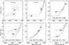 |
Fig. 1 Sample best fits to six of our binaries in the R vs. Teff diagram. Evolutionary tracks and observations for the primary in each system are represented with solid lines and open circles, while dashed lines and open squares are used for the secondary. Small dots indicate the best-fit location on each track and are always within the measurement uncertainties. |
4. Results
As can be inferred from the properties in Table B.1, or more directly from Fig. 1, some of our systems are in very rapid phases of evolution where ambiguities can sometimes occur as to the location of the components in the H-R (or radius vs. temperature) diagram. An advantage of our manual adjustments over the blind grid fits is that they allow us to avoid inconsistencies, such as the primary appearing near the secondary in the R vs. Teff diagram in a less evolved state, because of observational errors. Additionally, a few of our binaries have measured primary and secondary masses that are close or indistinguishable within the uncertainties, but they have very different radii and temperatures. Manual inspection allowed us to identify several cases in which the published identities of the components are reversed (see Table B.1).
Our results for the best-fit overshooting parameters, mixing length parameters, bulk abundances, and mean ages are presented in Table 1, where the systems are listed in the same order as in Table B.1. Approximate uncertainties for these values were estimated through experiments in which we varied αov, αMLT, or Z and examined the goodness of fit, always requiring the component ages to be within about 5% of each other. The uncertainties are strong functions of the evolutionary state, as this determines how sensitive the predicted properties (R, Teff) are to the fitted parameters. Typical theoretical errors for αov were found to be ± 0.03 for evolved stars (giants) and ± 0.04 for main-sequence stars, in which overshooting has less of an influence. Mixing length parameters have larger uncertainties of ± 0.20 for each star. Abundance errors are typically 25–30% in Z. Also the Z errors are very strongly correlated with the uncertainties in αov and αMLT.
Fitted parameters for our sample of DLEBs.
A graphical representation of αov as a function of stellar mass appears in Fig. 2, which shows the primary and secondary components together. Typical uncertainties described above are indicated in the lower right corner for evolved and unevolved stars. A clear pattern is seen in αov with a significant rise up to about 2 M⊙ followed by little or no change beyond this mass. The size of the symbols has been drawn proportional to Z. While this conveys in a more visual way the fact that the higher mass stars in our sample are all metal poor (and belong to the LMC or SMC, as seen in Table B.1) and that most low-mass stars have higher abundances (they are typically solar neighbourhood field stars), we see no significant difference in αov with Z at a given mass, at least in the present sample. The straight dashed lines in the figure delineate the apparent trend with mass. Four systems (V885 Cyg, χ2 Hya, VV Crv, and YZ Cas) have best fits yielding component ages that are different by more than 5%. The age discrepancies are7%, 15%, 15%, and 29%, respectively. The most egregious case of YZ Cas has been notoriously difficult to fit in the past, and remains so despite the recent observational efforts by Pavlovski et al. (2014), who redetermined the masses, radii, temperatures, and chemical composition. These four peculiar systems are represented with triangles in Fig. 2, but otherwise seem to follow the same trend as the other binaries. Also, as noted earlier, the primary components of OGLE-LMC-ECL-CEP-0227, OGLE-LMC-ECL-CEP-2532, and LMC-562.05-9009 are classical Cepheids (the first and last are fundamental-mode pulsators, and the second is a first-overtone pulsator), although again their overshooting parameters do not seem out of the ordinary for their mass.
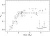 |
Fig. 2 Semi-empirical determination of the overshooting parameter αov as a function stellar mass for the stars in the 33 systems of our sample. Primary and secondary components are plotted together. The size of the points is proportional to Z, the bulk composition (metal-poor stars have smaller symbols). Stars indicated with triangles are those in which the inferred age difference within the binary exceeds our 5% tolerance (see text), but which give otherwise acceptable fits to the observations. Typical error bars for dwarfs and giants are shown on the bottom right. |
As mentioned before, our manual fits to the observations yield Z values that are often rather different from the corresponding spectroscopically measured composition for systems in which this is available. We show this in Fig. 3, where we transformed the fitted values of Z to the corresponding [Fe/H] measure assuming solar-scaled abundances and Z⊙ = 0.0189 to enable a more direct comparison in the observational plane. We also segregated the systems from the LMC, the SMC, and the field, as stars within these groups tend to have similar measured abundances. Only about half of the systems in our sample have a measured composition (see Table B.1).
Our fitted Z values (open circles) are often systematically lower than the corresponding spectroscopic [Fe/H] values (most noticeably in the LMC systems), sometimes by as much as a factor of two or three. In many cases this is well beyond the formal observational uncertainties. The reasons for this are unclear. Unrecognized biases in the measured [Fe/H] values or in the temperatures (which would need to be too hot by some 150 or 200 K, depending on the system) could explain these differences, but they would have to be systematic in nature as no instances of significantly overestimated best-fit Z values were found. We also investigated the impact of the abundance scale in our models. Tests showed that changing the reference solar abundances from those of Grevesse & Sauval (1998) to those of Asplund et al. (2009) does not make a significant difference in the corresponding fitted Z values. It is also possible that some of our objects (particularly the more metal-poor objects) are enhanced in α elements so that [α/ Fe] > 0, which would change the way we convert the model-fitted Z values to the inferred model-fitted [Fe/H] values shown in Fig. 3 (e.g. D’Antona et al. 2013). However, this effect goes in the wrong direction to explain what we see. Additional tests indicate that it is in fact possible to match the measured [Fe/H] values but only at the price of increasing αMLT to values significantly larger than 2.0, and even approaching 3.0 in some cases. There is no precedent for such high values of the mixing length parameter, however. Finally, it may also be that the discrepancy illustrated in the figure has to do with one or more of the physical ingredients in the models. A comparison of our fitted Z values with those fitted by others for systems where this check is possible gave mixed results: in some cases there is agreement, but in others our values are either higher or lower.
A closer look at the results in Table 1 seems to indicate a slight tendency for the fitted αMLT values to be higher in the LMC and SMC compared to the field binaries. The Magellanic Cloud populations are more metal poor than the field, on average, suggesting there may be a dependence of the mixing length parameter on metallicity. We note, however, that this apparent trend of higher αMLT values at lower abundances is opposite to that reported by Bonaca et al. (2012), who based their study on measured seismic oscillation frequencies in a sample of single dwarf and subgiant stars observed by the Kepler spacecraft. There are significant differences between their study and our study, which makes it difficult to pinpoint the reason(s) for the disagreement. For example, the stellar masses and radii in our analysis are strictly empirical (model independent) as they were derived from DLEBs, whereas those of Bonaca et al. (2012) were inferred from an initial fit to stellar evolution models, and used again in a subsequent fit to infer αMLT. Additionally, the Teff, [Fe/H], and log g ranges in our sample are all considerably larger than in the asteroseismic sample. In particular, Bonaca et al. (2012) have only one star with log g< 3.6, while our sample contains many. In fact, it is possible that the tentative differences we see in αMLT between the field binaries and the LMC/SMC binaries are related in part to evolutionary effects, as all of our systems in the LMC/SMC are red giants, in addition to being metal poor. Deficiencies in the stellar evolution models that may influence the fitted αMLT values cannot be ruled out at the present time (particularly in light of the fitted/measured abundance discrepancy discussed above), and the same holds for potential systematic errors in the measurement of Teff and/or [Fe/H], as noted earlier. For these reasons it may be premature to claim a firm detection of a correlation between αMLT and [Fe/H] or log g, although the hints we see certainly warrant further investigation.
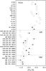 |
Fig. 3 Comparison between the available measured metallicities for the DLEBs in our sample (points with error bars) and the best-fit metallicities from our modelling (open circles), converted from Z to [Fe/H] as described in the text. Within each subgroup the binary systems are sorted as in Table B.1 by decreasing primary mass. |
5. Discussion
The dependence of the overshooting parameter αov on stellar mass presented in Fig. 2 is much more clearly established than in previous work, including that of Ribas et al. (2000) and Claret (2007), which suffered from a lack of suitable binary systems. Not only is the overall size of our binary list significantly larger, but the critical 1.2–2.0 M⊙ range in which αov ramps up from zero to an apparent maximum is much better sampled as well. The negative results of some of the more recent DLEB studies that did not see any mass dependence of αov can generally be understood in terms of the binary systems they used. For instance, of the four objects examined by Meng & Zhang (2014), some are similar regarding their component masses and this makes the sample effectively smaller. Furthermore, overshooting is assumed to be the same for the two components in each system, which would make it more difficult to detect any real change as a function of mass, especially since those binaries all have mass ratios that are significantly different from unity. For reasons that are not understood, unequal binaries such as these tend to be problematic to model, as we ourselves have found for χ2 Hya, VV Crv, and YZ Cas, which are three of the four objects in the Meng & Zhang (2014) sample. A similar modelling challenge was mentioned earlier for the unequal-mass binary V380 Cyg, which weighed heavily in the results of Ribas et al. (2000). The stars analysed by Stancliffe et al. (2015), on the other hand, cover a fairly wide range of masses, although most are clustered around 2 M⊙ and several are relatively unevolved and are therefore less sensitive to the effects of overshooting.
An interesting feature of our sample is that it spans a wide range of measured metallicities equivalent to a full factor of ten, from [Fe/H] of −1.01 to + 0.01. Despite this, we are unable to discern any dependence of αov on Z at a given mass, suggesting perhaps that the precision of our αov determinations would need to be considerably better to detect such an effect, if it exists, or that the sample needs to be even larger.
Many current stellar evolution models implement overshooting with a built-in dependence on stellar mass (and sometimes metallicity), even though the exact shape of that dependence has so far been poorly constrained by observations, except in the general sense that overshooting is irrelevant below 1.1–1.3 M⊙, then grows, and seems to level off at some larger mass. The top panel of Fig. 4 shows how some of those model prescriptions fare against our new results. In the Demarque et al. (2004) overshooting implementation the rise in αov from zero is steeper than indicated by our measurements, but eventually reaches a similar maximum around 0.2. The Pietrinferni et al. (2004) formula appears to have the right slope, but the rise starts and ends at lower masses. The models of Mowlavi et al. (2012) use a recipe for αov that grows to only half the peak value indicated by our analysis. It is worth mentioning here that our measurements of αov are semi-empirical in nature because they are based on the observed properties of binary systems but they also depend on models, specifically the Granada series of Claret (2004, 2012). Although this may suggest our results have limited applicability, the key physical ingredients in most modern stellar evolution codes (standard mixing-length approximation, radiative opacities, etc.) are rather similar, so we expect our conclusions to be valid for other models as well.
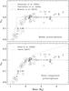 |
Fig. 4 Our semi-empirical determinations of αov as a function of stellar mass, compared with published prescriptions. Symbols are as in Fig. 2, with sizes drawn here proportional to the surface gravity log g of each star. Top: mass dependence of αov adopted in some recent grids of stellar evolution models. Bottom: comparison with previous semi-empirical relationships by Ribas et al. (2000) and Claret (2007). |
Previous semi-empirical results are compared with our results in the lower panel of Fig. 4. As noted earlier, the Ribas et al. (2000) mass dependence of αov is steeper than indicated by our measurements, while that of Claret (2007), which was based on a smaller sample than ours and had much larger uncertainties in αov, is fairly close to the trend indicated by our results. This is the case except possibly at the very lowest masses, where that study had only one star (the secondary of YZ Cas). This study also suggested a slight increase in αov for stars more massive than 10 M⊙, a regime our sample does not address.
An assumption that is implicit in the present work, and indeed in all stellar evolution codes we are aware of, is that αov does not depend on the evolutionary state of the star at a given mass, i.e. it does not vary with time. With the usual expression dov = αovHp for the distance travelled by convective cells above the boundary of the core, it is clear that dov changes as a star evolves because Hp does, but αov could well vary independently in some fashion (as speculated, e.g. by Torres et al. 2014). Our measurements allow a first look into this issue. In Fig. 4 we represented the αov measurements with symbols whose size is proportional to the surface gravity of the star (log g) to more easily distinguish dwarfs from giants. While most stars on the rising part of the αov versus mass trend (M< 2 M⊙) are main-sequence stars, some are low mass giants (smaller symbols), and there seems to be no significant difference between the overshooting parameters of dwarfs and giants of similar mass. The behaviour at higher masses cannot be addressed with the present sample for lack of sufficiently evolved main-sequence binaries with M> 2 M⊙.
The clear evidence from our semi-empirical measurements that the influence of overshooting initially rises as the mass increases from about 1.2 M⊙ carries some interest in itself from the theoretical point of view, as it must contain quantitative information about the implied growth of the convective core. We investigated this using the same best-fit models for the stars in our sample from which we obtained αov. As the size (mass) of the core also changes with time as stars evolve, we chose to eliminate the time dependence by extracting the mass of the convective core at the ZAMS from each model used to generate Fig. 2, and we then normalized it to the total mass of the star. The results for the fractional core mass Qc obtained in this way are shown in the top panel of Fig. 5, shown as a function of stellar mass. For reference we added a solid curve representing the predicted change in Qc in the absence of overshooting, also at the ZAMS. While this last curve clearly indicates, as expected, that the core mass grows with stellar mass even without overshooting, the increase is considerably more pronounced with overshooting, and our semi-empirical measurements of Qc allow us to quantify the degree to which this is the case. The lower panel shows the fractional increase in Qc as a function of stellar mass, and indicates that for stars beyond about 2 M⊙ it converges towards an enlargement of about 50% above the core mass that would result in the absence of overshooting. This differential increase raises additional questions of interest. What is the maximum possible size of the convective core for a given stellar mass? How does αov influence the size of the core at different stellar masses? With relatively simple arguments and the use of the virial theorem it can be shown that there is in fact an upper limit to the size of the mixed core, implying a limit to αov, as we see from our measurements. Thus, it is possible to understand the general features of Fig. 2, at least over the mass range explored here. The details of these calculations are provided in the Appendix.
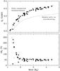 |
Fig. 5 Top: semi-empirical values Qc of the convective core mass at the ZAMS (normalized to the total mass) for each of the stars in our sample. Triangles represent components of systems with age differences exceeding 5%. The dashed line is a third-order polynomial fit drawn to guide the eye. The solid line shows the trend of Qc with mass for solar-metallicity ZAMS models having αov = 0, for reference. Bottom: fractional increase in Qc over that indicated by the solid line in the top panel, expressed as a percentage. |
6. Conclusions
We have used the measured masses, radii, and effective temperatures of more than 30 carefully selected double-lined eclipsing binary systems to infer semi-empirical values of αov for each of the components by comparison with stellar evolution models. Importantly, the sample includes a substantial number of highly evolved systems (red giants, mostly in the LMC and SMC) that are more sensitive to the effects of overshooting. This significantly larger and more suitable sample compared to previous studies has allowed us to calibrate the dependence of overshooting on stellar mass. This dependence has traditionally been assumed to be present, and has been implemented in various ways in current stellar evolution models, but until now it has not been well constrained by observations. We find a clear and fairly linear increase in αov beginning at about 1.2 M⊙ and reaching αov ~ 0.2 around 2.0 M⊙, with little change beyond this mass up to the limit of our sample (4.4 M⊙). This trend is similar to, but much better defined than that proposed by Claret (2007), and differs in various ways from prescriptions currently used in other model sets that adopt the same formulation for the extension of the convective core as dov = αovHp. Our results may serve as a guide for future implementations of overshooting in model grids. We also find no significant variance in αov for giants and dwarfs at a given mass, suggesting αov does not depend very strongly on evolutionary state. Three of our LMC systems are Cepheids, although no significant difference is found in their αov values either compared to other stars of similar mass. The main features of the αov versus mass trend, which is the main result of this work, can be understood by simple physical arguments as laid out in Appendix A.
We also made use of the same best-fit models for our 33 binary systems to calibrate the extent of the convective core as a function of stellar mass. We find that for stars more massive than about 2 M⊙ the growth of the fractional core mass Qc converges to a level of about 50% above the values predicted by models without overshooting.
All of our binary systems yield satisfactory fits when compared with the models, with the exception of four (V885 Cyg, χ2 Hya, VV Crv, and YZ Cas) in which the component ages differ by more than 5% (particularly YZ Cas), although their other properties are well matched. The last three of these have mass ratios that are appreciably different from unity; the fact that another similarly unequal system (V380 Cyg) has also been difficult to model in past studies by other investigators suggests either unrecognized measurement errors in such systems, or some other problem that has yet to be identified, and is perhaps related to their origin.
Half of the binaries in our sample have a spectroscopically measured [Fe/H] abundance in the literature. In about half of those cases we find curious systematic differences between the measured composition and the Z values from our best fits, after conversion to the [Fe/H] scale: the fitted values tend to be smaller, often significantly so. Most of these systems belong to the LMC. There are no examples with opposite discrepancies of much significance, and the reasons for this are not understood. In some cases other authors have found similar deviations, although this has not been emphasized. There are also hints in our sample that the fitted αMLT values may be higher for stars that are more metal poor and/or more evolved, although this may be related to the Z differences just noted, and needs to be investigated further.
Although our sample is much larger than previous lists of binaries used to calibrate overshooting, it is still limited in that it contains no systems with component masses beyond 4.4 M⊙. Therefore, we are unable to verify claims by other investigators about possible changes in αov for more massive stars. While our objects do cover a range of about a factor of ten in metal abundance, and we find no significant dependence of αov on Z within our measurement uncertainties, a larger metallicity range is desirable to confirm this conclusion and perhaps track down the deviations mentioned above.
Acknowledgments
We thank the anonymous referee for helpful comments on the original manuscript. The Spanish MEC (AYA2015-71718-R) is gratefully acknowledged for its support during the development of this work. G.T. acknowledges partial support from the NSF through grant AST-1509375. This research has made use of the SIMBAD database, operated at the CDS, Strasbourg, France, and of NASA’s Astrophysics Data System Abstract Service.
References
- Aerts, C. 2013, in Setting a New Standard in the Analysis of Binary Stars, eds. K. Pavlovski, A. Tkachenko, & G. Torres, EAS Pub. Ser., 64, 323 [Google Scholar]
- Aerts, C. 2015, in New Windows on Massive Stars: Asteroseismology, Interferometry, and Spectropolarimetry, Proc. International Astronomical Union, IAU Symp., 307, 154 [NASA ADS] [Google Scholar]
- Andersen, J. 1991, A&ARv, 3, 91 [NASA ADS] [CrossRef] [Google Scholar]
- Andersen, J., Clausen, J. V., & Nordström, B. 1990, A&A, 363, 33 [Google Scholar]
- Asplund, M., Grevesse, N., Sauval, A. J., & Scott, P. 2009, ARA&A, 47, 481 [NASA ADS] [CrossRef] [Google Scholar]
- Böhm-Vitense, E. 1958, Z. Astrophys., 46, 108 [Google Scholar]
- Bonaca, A., Tanner, J. D., Basu, S., et al. 2012, ApJ, 755, L12 [NASA ADS] [CrossRef] [Google Scholar]
- Bressan, A. 1992, Mem. Soc. Astron. It., 63, 25 [NASA ADS] [Google Scholar]
- Bressan, A., Marigo, P., Girardi, L., et al. 2012, MNRAS, 427, 127 [NASA ADS] [CrossRef] [Google Scholar]
- Claret, A. 2004, A&A, 424, 919 [NASA ADS] [CrossRef] [EDP Sciences] [Google Scholar]
- Claret, A. 2007, A&A, 475, 1019 [NASA ADS] [CrossRef] [EDP Sciences] [Google Scholar]
- Claret, A. 2012, A&A, 541, A113 [NASA ADS] [CrossRef] [EDP Sciences] [Google Scholar]
- Claret, A., & Giménez, A. 1991, A&A, 244, 319 [NASA ADS] [Google Scholar]
- Claret, A., & Giménez, A. 2010, A&A, 519, A57 [NASA ADS] [CrossRef] [EDP Sciences] [Google Scholar]
- D’Antona, F., Caloi, V., D’Erole, A., et al. 2013, MNRAS, 434, 1138 [NASA ADS] [CrossRef] [Google Scholar]
- Deheuvels, S., Brandao, I., Silva Aguirre, V., et al. 2016, A&A, 589, A93 [NASA ADS] [CrossRef] [EDP Sciences] [Google Scholar]
- Demarque, P., Woo, J.-H., Kim, Y.-C., & Yi, S. K. 2004, ApJS, 155, 667 [NASA ADS] [CrossRef] [Google Scholar]
- Elgueta, S. S., Graczyk, D., Gieren, W., et al. 2016, AJ, in press [Google Scholar]
- Fekel, F. C., Henry, G. W., & Sowell, J. R. 2013, AJ, 146, 146 [NASA ADS] [CrossRef] [Google Scholar]
- Ferguson, J. W., Alexander, D. R., Allard, F., et al. 2005, ApJ, 623, 585 [NASA ADS] [CrossRef] [Google Scholar]
- Gieren, W., Pilecki, B., Pietrzyński, G., et al. 2015, ApJ, 815, 28 [NASA ADS] [CrossRef] [Google Scholar]
- Graczyk, D., Pietrzyński, G., Thompson, I. B., et al. 2012, ApJ, 750, 144 [NASA ADS] [CrossRef] [Google Scholar]
- Graczyk, D., Pietrzyński, G., Thompson, I. B., et al. 2014, ApJ, 780, 59 [NASA ADS] [CrossRef] [Google Scholar]
- Grevesse, N., & Sauval, A. J. 1998, Space Sci. Rev., 85, 161 [NASA ADS] [CrossRef] [Google Scholar]
- Hełminiak, K. G., Graczyk, D., Konacki, M., et al. 2015, MNRAS, 448, 1945 [NASA ADS] [CrossRef] [Google Scholar]
- Iglesias, C. A., & Rogers, F. J. 1996, ApJ, 464, 943 [NASA ADS] [CrossRef] [Google Scholar]
- Lastennet, E., & Valls-Gabaud, D. 2002, A&A, 396, 551 [NASA ADS] [CrossRef] [EDP Sciences] [Google Scholar]
- Meng, Y., & Zhang, Q. S. 2014, ApJ, 787, 127 [NASA ADS] [CrossRef] [Google Scholar]
- Mowlavi, N., Eggenberger, P., Meynet, G., et al. 2012, A&A, 541, A41 [NASA ADS] [CrossRef] [EDP Sciences] [Google Scholar]
- Nieuwenhuijzen, H., & de Jagger, C. 1990, A&A, 231, 134 [NASA ADS] [Google Scholar]
- Pavlovski, K., Southworth, J., Kolbas, V., & Smalley, B. 2014, MNRAS, 438, 590 [NASA ADS] [CrossRef] [Google Scholar]
- Paxton, B., Bildsten, L., Dotter, A., et al. 2011, ApJS, 192, 3 [Google Scholar]
- Pietrinferni, A., Cassisi, S., Salaris, M., & Castelli, F. 2004, ApJ, 612, 168 [NASA ADS] [CrossRef] [Google Scholar]
- Pietrzyński, G., Thompson, I. B., Gieren, W., et al. 2010, Nature, 468, 542 [NASA ADS] [CrossRef] [PubMed] [Google Scholar]
- Pietrzyński, G., Graczyk, D., Gieren, W., et al. 2013, Nature, 495, 76 [NASA ADS] [CrossRef] [PubMed] [Google Scholar]
- Pilecki, B., Graczyk, D., Pietrzyński, G., et al. 2013, MNRAS, 436, 953 [NASA ADS] [CrossRef] [Google Scholar]
- Pilecki, B., Graczyk, D., Gieren, W., et al. 2015, ApJ, 806, 29 [NASA ADS] [CrossRef] [Google Scholar]
- Pols, O. R., Tout, C. A., Eggleton, P. P., & Han, Z. 1995, MNRAS, 274, 964 [NASA ADS] [CrossRef] [Google Scholar]
- Reimers, D. 1977, A&A, 61, 217 [NASA ADS] [Google Scholar]
- Ribas, I. 1999, Ph.D. Thesis, Universitat de Barcelona [Google Scholar]
- Ribas, I., Jordi, C., & Giménez, A. 2000, MNRAS, 318, 55 [Google Scholar]
- Roxburgh, I. W. 1965, MNRAS, 130, 223 [NASA ADS] [Google Scholar]
- Roxburgh, I. W. 1978, A&A, 65, 281 [NASA ADS] [Google Scholar]
- Roxburgh, I. W. 1989, A&A, 211, 361 [NASA ADS] [Google Scholar]
- Sandberg Lacy, C. H., & Fekel, F. C. 2011, AJ, 142, 185 [NASA ADS] [CrossRef] [Google Scholar]
- Saslaw, W. C., & Schwarzschild, M. 1965, ApJ, 142, 1468 [NASA ADS] [CrossRef] [Google Scholar]
- Schaller, G., Schaerer, D., Meynet, G., & Maeder, A. 1992, A&AS, 96, 269 [Google Scholar]
- Stancliffe, R. J., Fossati, L., Passy, J.-C., & Schneider, F. R. N. 2015, A&A, 575, A117 [NASA ADS] [CrossRef] [EDP Sciences] [Google Scholar]
- Stothers, R. B., & Chin, C.-W. 1991, ApJ, 381, L67 [NASA ADS] [CrossRef] [Google Scholar]
- Stothers, R. B., & Chin, C.-W. 1992, ApJ, 390, 136 [NASA ADS] [CrossRef] [Google Scholar]
- Tkachenko, A., Degroote, P., Aerts, C., et al. 2014, MNRAS, 438, 3093 [NASA ADS] [CrossRef] [Google Scholar]
- Torres, G., Andersen, J., & Giménez, A. 2010, A&ARv, 18, 67 [Google Scholar]
- Torres, G., Vaz, L. P. R., Lacy, C. H. S., & Claret, A. 2014, AJ, 147, 36 [NASA ADS] [CrossRef] [Google Scholar]
- Torres, G., Claret, A., Pavlovski, K., & Dotter, A. 2015, ApJ, 807, 26 [NASA ADS] [CrossRef] [Google Scholar]
- Valle, G., Dell’Omodarme, M., Prada Moroni, P. G., & Degl’Innocenti, S. 2016, A&A, 587, A16 [NASA ADS] [CrossRef] [EDP Sciences] [Google Scholar]
- VandenBerg, D. A., Bergbusch, P. A., & Dowler, P. 2006, ApJS, 162, 375 [NASA ADS] [CrossRef] [MathSciNet] [Google Scholar]
Appendix A: A study of extra mixing using the virial theorem
In order to investigate the consequences of extra mixing on the internal physical conditions of a star, we have selected a model of a 3 M⊙ star with composition X = 0.751 and Z = 0.003 that is representative of our observational sample. A first point of interest is the issue of how the extra mixing depends on the αov parameter, defined as in the main text by dov = αovHp, where Hp is the pressure scale height. Figure A.1 shows the behaviour of the fractional mixed core mass Qc = Mc/M as a function of αov at the ZAMS, in which Mc is the mass of the convective core and M the total mass of the star. It can be seen that up to αov ≈ 1.0 the increase in Qc is essentially linear, and tests reveal that the slope dQc/dαov ≈ 0.3 is almost independent of stellar mass. For higher αov values the figure suggests that a limit to the size of the mixed core is eventually reached, such that for αov higher than about 2.5 the fractional core mass Qc is practically independent of the overshooting parameter. For a closer look into this limit we make use here of the virial theorem, a very useful but frequently overlooked analytical tool for stellar physics.
The virial theorem for a star may be written as 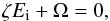 (A.1)in which
  is the total internal energy,
 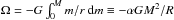 is the gravitational potential energy, and R is the stellar radius. In addition, for an ideal gas we have u = cvT and ζu = 3P/ρ = 3(γ−1), and γ = cP/cv, where u is the specific internal energy, P the pressure, T the temperature, and cv and cP are the specific heats at constant volume and constant pressure.
However, Eq. (A.1) derives from the hydrostatic differential equation assuming that the pressure at the boundary vanishes. In the more general case we may write the virial for the mixed core as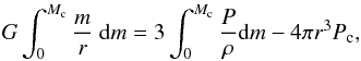 (A.2)where Pc denotes the pressure at the boundary of the core. Equation (A.1) then becomes
  (A.3)Equation (A.3) may be used to study the consequences of the extension of the core due to extra mixing under the condition of hydrostatic equilibrium. To proceed we assume for simplicity a non-degenerate ideal gas. As the extra mixing increases (corresponding to higher adopted values of αov in our framework), the pressure at the border of the core decreases. We may estimate the maximum extent of the extra mixing (in terms of the radial coordinate and pressure) by solving dP/dr = 0, that is,
  (A.4)From this, the critical radius rcrit is given by
  (A.5)where μ is the mean molecular weight, k is the Boltzmann constant, and
  . Correspondingly, there is a critical value for the pressure at the border of the mixed core, Pcrit, which can hydrostatically support the weight of the envelope as follows:
  (A.6)The expression above shows that Pcrit decreases as the core mass increases, as expected. On the other hand, the pressure at the bottom of the envelope is
  . The condition of hydrostatic equilibrium at the interface implies that
  (A.7)The pressure at the bottom of the envelope can be extracted from the models shown in Fig. A.1, and compared with Pcrit. This comparison appears in Fig. A.2. Despite the simplicity of the assumptions adopted for our use of virial theorem (ideal non-degenerate gas, no radiation pressure, non-rotating models, etc.), the results in Fig. A.2 are in good agreement with those shown in Fig. A.1: the curves in Fig. A.2 meet at approximately the same value of αov at which the trend in Fig. A.1 levels off. Applying Eq. (A.7) to Fig. A.2 we may infer a limit to the size of the mixed core (for the present case, Qc,max ≈ 0.75) and consequently a critical value for αov around 2.0–2.5, although given our assumptions and simplifications, this limit value could be as low as αov ≈ 1.5. Mutatis mutandis, we expect the same should occur for other masses typical of our observational sample. The critical values of the radius and pressure are also influenced by the initial chemical composition, not only through changes in the internal structure (for example, the convective core for a Z = 0.02 model is slightly smaller than for one with Z = 0.003), but also directly in the calculation of Pcrit (see above).
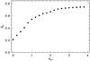 |
Fig. A.1 Dependence of the fractional mass of the mixed core as a function of the overshooting parameter αov, for models with 3 M⊙ and composition X = 0.751 and Z = 0.003. Note the linear behaviour of Qc for αov ≤ 1.0. |
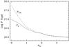 |
Fig. A.2 Pressure on a logarithmic scale at the bottom of the envelope (solid line), compared with the critical pressure Pcrit given by equation A.6 (dashed line), as a function of the overshooting parameter αov. The models are the same as those in Fig. A.1. |
Appendix B: Additional table
Binaries systems in our sample.
All Tables
All Figures
|
Fig. 1 Sample best fits to six of our binaries in the R vs. Teff diagram. Evolutionary tracks and observations for the primary in each system are represented with solid lines and open circles, while dashed lines and open squares are used for the secondary. Small dots indicate the best-fit location on each track and are always within the measurement uncertainties. |
| In the text | |
|
Fig. 2 Semi-empirical determination of the overshooting parameter αov as a function stellar mass for the stars in the 33 systems of our sample. Primary and secondary components are plotted together. The size of the points is proportional to Z, the bulk composition (metal-poor stars have smaller symbols). Stars indicated with triangles are those in which the inferred age difference within the binary exceeds our 5% tolerance (see text), but which give otherwise acceptable fits to the observations. Typical error bars for dwarfs and giants are shown on the bottom right. |
| In the text | |
|
Fig. 3 Comparison between the available measured metallicities for the DLEBs in our sample (points with error bars) and the best-fit metallicities from our modelling (open circles), converted from Z to [Fe/H] as described in the text. Within each subgroup the binary systems are sorted as in Table B.1 by decreasing primary mass. |
| In the text | |
|
Fig. 4 Our semi-empirical determinations of αov as a function of stellar mass, compared with published prescriptions. Symbols are as in Fig. 2, with sizes drawn here proportional to the surface gravity log g of each star. Top: mass dependence of αov adopted in some recent grids of stellar evolution models. Bottom: comparison with previous semi-empirical relationships by Ribas et al. (2000) and Claret (2007). |
| In the text | |
|
Fig. 5 Top: semi-empirical values Qc of the convective core mass at the ZAMS (normalized to the total mass) for each of the stars in our sample. Triangles represent components of systems with age differences exceeding 5%. The dashed line is a third-order polynomial fit drawn to guide the eye. The solid line shows the trend of Qc with mass for solar-metallicity ZAMS models having αov = 0, for reference. Bottom: fractional increase in Qc over that indicated by the solid line in the top panel, expressed as a percentage. |
| In the text | |
|
Fig. A.1 Dependence of the fractional mass of the mixed core as a function of the overshooting parameter αov, for models with 3 M⊙ and composition X = 0.751 and Z = 0.003. Note the linear behaviour of Qc for αov ≤ 1.0. |
| In the text | |
|
Fig. A.2 Pressure on a logarithmic scale at the bottom of the envelope (solid line), compared with the critical pressure Pcrit given by equation A.6 (dashed line), as a function of the overshooting parameter αov. The models are the same as those in Fig. A.1. |
| In the text | |
Current usage metrics show cumulative count of Article Views (full-text article views including HTML views, PDF and ePub downloads, according to the available data) and Abstracts Views on Vision4Press platform.
Data correspond to usage on the plateform after 2015. The current usage metrics is available 48-96 hours after online publication and is updated daily on week days.
Initial download of the metrics may take a while.