| Issue |
A&A
Volume 592, August 2016
|
|
|---|---|---|
| Article Number | A141 | |
| Number of page(s) | 10 | |
| Section | Atomic, molecular, and nuclear data | |
| DOI | https://doi.org/10.1051/0004-6361/201628656 | |
| Published online | 17 August 2016 | |
Energy levels and transition rates for helium-like ions with Z = 10–36⋆
1 Division of Mathematical Physics, Department of Physics, Lund University, Box 118, 221 00 Lund, Sweden
e-mail: This email address is being protected from spambots. You need JavaScript enabled to view it.
2 Shanghai EBIT Lab, Institute of Modern Physics, Department of Nuclear Science and Technology, Fudan University, Shanghai 200433, PR China
e-mail: This email address is being protected from spambots. You need JavaScript enabled to view it.
3 Applied Ion Beam Physics Laboratory, Fudan University, Key Laboratory of the Ministry of Education, Shanghai 200433, PR China
4 Hebei Key Lab of Optic-electronic Information and Materials, The College of Physics Science and Technology, Hebei University, Baoding 071002, PR China
5 Institute of Applied Physics and Computational Mathematics, Beijing 100088, PR China
6 Center for Applied Physics and Technology, Peking University, Beijing 100871, PR China
7 Collaborative Innovation Center of IFSA (CICIFSA), Shanghai Jiao Tong University, Shanghai 200240, PR China
Received: 7 April 2016
Accepted: 31 May 2016
Abstract
Aims. Helium-like ions provide an important X-ray spectral diagnostics in astrophysical and high-temperature fusion plasmas. An interpretation of the observed spectra provides information on temperature, density, and chemical compositions of the plasma. Such an analysis requires information for a wide range of atomic parameters, including energy levels and transition rates. Our aim is to provide a set of accurate energy levels and transition rates for helium-like ions with Z = 10–36.
Methods. The second-order many-body perturbation theory (MBPT) was adopted in this paper. To support our MBPT results, we performed an independent calculation using the multiconfiguration Dirac-Hartree-Fock (MCDHF) method.
Results. We provide accurate energies for the lowest singly excited 70 levels among 1snl(n ≤ 6,l ≤ (n−1)) configurations and the lowest doubly excited 250 levels arising from the K-vacancy 2ln′l′(n′ ≤ 6,l′ ≤ (n′−1)) configurations of helium-like ions with Z = 10−36. Wavelengths, transition rates, oscillator strengths, and line strengths are calculated for the E1, M1, E2, and M2 transitions among these levels. The radiative lifetimes are reported for all the calculated levels.
Conclusions. Our MBPT results for singly excited n ≤ 2 levels show excellent agreement with other elaborate calculations, while those for singly excited n ≥ 3 and doubly excited levels show significant improvements over previous theoretical results. Our results will be very helpful for astrophysical line identification and plasma diagnostics.
Key words: atomic data / atomic processes
Full Tables 1 and 2 are only available at the CDS via anonymous ftp to cdsarc.u-strasbg.fr (130.79.128.5) or via http://cdsarc.u-strasbg.fr/viz-bin/qcat?J/A+A/592/A141
© ESO 2016
1. Introduction
Helium-like ions provide an important X-ray spectral diagnostics in astrophysical and high-temperature fusion plasmas (Gabriel & Jordan 1969; Gabriel 1972; Pradhan & Shull 1981; Porquet et al. 2001, 2010). Emission lines from the spectra of both singly and doubly excited helium-like ions are often observed in the spectra of solar, stellar, and other astrophysical plasmas (e.g., Walker & Rugge 1970; Seely & Feldman 1985; Phillips et al. 1993; Harra-Murnion et al. 1996; Feldman et al. 2000; Dere et al. 2001; Ness et al. 2003; Paerels & Kahn 2003; Phillips 2004; Landi & Phillips 2005; Güdel & Naz é 2009; Sylwester et al. 2010). Spectral lines of helium-like ions are also prominent features in the X-ray spectra of tokamak plasmas and laser-produced plasmas. These features arise from impurity elements (e.g., Hsuan et al. 1987; Bombarda et al. 1988; Beiersdorfer et al. 1995; Elton et al. 2000; Rosmej et al. 2002; Rice et al. 1987, 1999, 2000, 2014, 2015). The relative intensities of spectral lines from the n = 2 shell to the ground state have been widely used in temperature and density diagnostics for solar plasma (e.g., McKenzie et al. 1979; Wolfson et al. 1983; Keenan et al. 1984; Doyle & Keenan 1986) and tokamak plasmas (e.g., Källne et al. 1983; Keenan et al. 1989). Spectral lines decaying from doubly excited helium-like ions are essential in understanding the dielectronic recombination process of hydrogen-like ions. The lines that appear as hydrogen-like satellites are often observed in astrophysical plasmas, and the hydrogen-like satellite-to-resonance intensities can be used to measure electron temperatures in solar flares (Dubau et al. 1981; Parmar et al. 1981; Tanaka 1986; Pike et al. 1996). Furthermore, the high-n dielectronic recombination from the hydrogen-like ions can significantly affect some helium-like line ratios from low-lying (n = 2) transitions (Smith et al. 2001). The analysis of the observed spectra requires information for a wide range of atomic parameters, including energy levels and transition rates (Kallman & Palmeri 2007; Smith 2014).
There are many experimental studies of singly excited helium-like ions (for example, see references in Beiersdorfer et al. 1989; and Beiersdorfer & Brown 2015). The systematic theoretical studies are mostly confined to the n = 2 complex (e.g., Drake 1988; Chen et al. 1993; Cheng et al. 1994; Plante et al. 1994; Johnson et al. 1995; Cheng & Chen 2000; Artemyev et al. 2005). There are also some large-scale calculations involving n> 2 singly excited levels of helium-like ions. Johnson et al. (2002) presented transition wavelengths and rates for a limited set of electric-dipole (E1) transitions among 1snl (n ≤ 6, l ≤ 3) configurations of C V, N VI, O VII, Ne IX, Si XIII, and Ar XVII using a relativistic configuration-interaction (CI) approach. Savukov et al. (2003) extended the calculations to give a more complete treatment of E1 transitions and to include forbidden electric-quadrupole (E2), magnetic-dipole (M1), and magnetic-quadrupole (M2) transitions. Aggarwal et al. (2005, 2008, 2009, 2010, 2011, 2012a,b,c,d, 2013a,b) included level energies and multipole rates for transitions within 1snl (n ≤ 5, l ≤ (n−1)) configurations of helium-like ions with Z = 3−36 (except for Ne IX) using the GRASP code (Grant et al. 1980). However, we show below that because they treated correlation only in a limited way, their energies differ from the experimental values by more than 3 eV, which does not meet the accuracy requirement in the fitting of observed spectra (Kharchenko & Dalgarno 2001; Kallman & Palmeri 2007; Smith 2014; Beiersdorfer 2015).
The doubly excited states of helium-like ions have also been investigated in various experiments (O’Rourke et al. 2008; Nandi 2008; Nakano et al. 2012; Kasthurirangan et al. 2013). The newly developed X-ray free-electron lasers (FEL) provide a unique opportunity to investigate the behavior of inner-shell vacancy ions (Young et al. 2010; Bucksbaum et al. 2011; Düsterer et al. 2011; Kanter et al. 2011; Meyer et al. 2012). The theoretical studies of the K-vacancy doubly excited levels of helium-like ions are mostly based on non-relativistic theory or confined to some selected transitions within 2l2l′ and 2l3l′ configurations (Vainshtein & Safronova 1976, 1978, 1980, 1985; Dubau et al. 1981; Safronova & Senashenko 1977; Karim & Bhalla 1986; Mosnier et al. 1986; Cornille et al. 1990; Deng-Hong et al. 2006; Karim 2010; Kadrekar & Natarajan 2011; Natarajan & Kadrekar 2013; Natarajan 2014). The most recent and complete of these studies has been reported by Goryayev et al. (2006), who presented the wavelengths and radiative transition probabilities for transitions of 2l′2l′′−1s2l and 2l′3l′′−1s2l,1s3l in ions with Z = 6−36 using the Z-expansion method. However, some of the crucial radiative channels, such as all of the transitions between doubly excited levels and transitions decaying from 2lnl′(n> 3) configurations, are overlooked in that work, which are important in plasma modeling (Karim et al. 1992; Karim & Bhalla 1995; Yamamoto et al. 2005).
In this paper, our aim is to provide more complete and accurate atomic data of the helium isoelectronic sequence for Z = 10−36. By using the second-order many-body perturbation theory (MBPT) with the flexible atomic code (FAC; Gu 2008), we provide energies and radiative lifetimes for the 70 lowest singly excited levels of the 1snl(n ≤ 6,l ≤ (n−1)) configurations and the 250 lowest doubly excited levels of the 2ln′l′(n′ ≤ 6,l′ ≤ (n′−1)) configurations. In addition, wavelengths, transition rates, oscillator strengths, and line strengths are calculated for E1, E2, M1, and M2 transitions between these levels. To support our MBPT results, we have performed an independent calculation using the multiconfiguration Dirac-Hartree-Fock (MCDHF) method in the form of the latest version of the GRASP2K code (Jönsson et al. 2013) for some of the ions (Ne IX, Si XIII, Ar XVII, Ti XXI, Fe XXV and Zn XXIX). The quality and reliability of our MBPT values are assessed by extensive comparison with experimental and some other theoretical values.
2. Calculation
2.1. MBPT
The second-order MBPT approach (Lindgren 1974; Safronova et al. 1996), implemented by Gu (2005, 2006) in FAC has been used successfully to calculate atomic parameters with high accuracy (Gu 2007; Gu et al. 2011; Wang et al. 2014; Fei et al. 2014; Guo et al. 2015; Wang et al. 2015; Si et al. 2015a,b). Here we briefly describe the theory.
In the MBPT method implemented in FAC, the no-pair Dirac-Coulomb-Breit Hamiltonian (HDCB; Sucher 1980) is used for anN-electron atom or ion, in which the frequency-independent Breit interaction has been included. The key feature of the MBPT approach is to divide the Hilbert space of the full Hamiltonian into a model space M and an orthogonal space N. The eigenvalues in second order of the full Hamiltonian are obtained through solving the first-order eigenvalue problem of the non-Hermitian effective Hamiltonian in the model space M. By using this method, the electron correlations within M are included to all orders, while the interaction between M and N is taken into account to second order with the perturbation method. The model space M here contains all the configurations we are interested in, that is all the possible configurations of 1snl(n ≤ 6,l ≤ (n−1)) and 2ln′l′(n′ ≤ 6,l′ ≤ (n′−1)). The orthogonal space N contains all configurations that are formed by single and double (SD) excitations from the M space, where a finite boundary is used to discretize the continuum states.
Finally, the vacuum polarization effects are taken into account by including the Uehling potential, and electron self-energies are included using a screened hydrogenic formula. The effects of finite nuclear size are calculated by using the nuclear potential for a finite hard sphere, and the nuclear recoil is included by adding the corresponding matrix elements to HDCB (Parpia et al. 1992).
2.2. MCDHF
In the MCDHF method implemented in GRASP2K code (Jönsson et al. 2013), the Hamiltonian is the Dirac-Coulomb Hamiltonian HDC. The atomic state functions (ASFs) Ψ(γPJ) are approximated by expansions over jj-coupled configuration state functions (CSFs) Φ(γPJ). Based on the so-called extended optimal level (EOL) scheme (Dyall et al. 1989) with the standard level weights of several states, the radial parts of the Dirac orbitals and the expansion coefficients were both optimized to self-consistency in the relativistic self-consistent field procedure. In the subsequent configuration-interaction calculation (McKenzie et al. 1980), the Breit interaction was computed in the low-frequency limit by multiplying the frequency with a scale factor of 10-6, while the other small corrections such as VP and SE were included in a similar fashion to the approach in FAC.
We used a restrictive active space method to generate a CSF expansion. In this method, the electrons from the occupied orbitals are excited to unoccupied orbitals in an active set. The orbital was increased systematically to monitor the convergence of the calculation. Since the orbitals with the same principal quantum number n have near similar energies, the active set is expanded in layers of n. For the singly excited 1snl(n ≤ 6, l ≤ (n−1)) states, CSFs of the forms nln′l′ (n,n′ ≤ 10,l,l′ ≤ 6) are included in the final active set.
3. Results
3.1. Energy levels
In Table 1, we list our calculated fine-structure energies of 1snl(n ≤ 6,l ≤ (n−1)) and 2ln′l′(n′ ≤ 6,l′ ≤ (n′−1)) configurations of helium-like ions with Z = 10−36 obtained from the MBPT approach as well as our MCDHF values for singly excited levels of Ne IX, Si XIII, Ar XVII, Ti XXI, Fe XXV, and Zn XXIX and the NIST compiled values (Kramida et al. 2015). The jj-coupling and LS-coupling identifications are both listed. In the last column of Table 1, we give the LS-coupling compositions of the levels. It is clear that the mixings in many cases are very strong, especially for the doubly excited levels. For the LS-label of different levels, we used the CSF-component with the highest weight, and when this had been used to represent lower levels, we based the labeling on the second largest component.
We compare our computed 1890 singly excited levels to the 1028 energies provided by the NIST database (Kramida et al. 2015) in Table 1, and the deviations as a function of Z for the 1s2l group are shown in Fig. 1. Some obvious anomalies are evident in the sequence, especially in the range Z = 31−36, as well as for some fairly highly excited levels in other ions (e.g., 1s3d1D2, 1s4f1F3 and 1s5f1F3 in Ne IX). This clearly calls for a re-evaluation of the NIST values. Except for these irregularities, our MBPT energy levels are mostly lower than the NIST values by about 50 ppm.
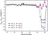 |
Fig. 1 Comparison of our MBPT energies to NIST values (Kramida et al. 2015) as a function of Z for 1s2l configurations. The horizontal lines indicate differences of ±1000 cm-1. |
Level designations, excitation energies (in cm-1), and lifetimes (τ in s) for the 321 levels arising from the 1snl(n ≤ 6,l ≤ (n−1)) and 2ln′l′(n′ ≤ 6,l′ ≤ (n′−1)) configurations of helium-like ions with Z = 10−36.
Wavelengths (λ, in Å), transition rates (A, in s-1), oscillator strengths (f, dimensionless), and line strengths (S, in a.u.) for transitions among 1snl(n ≤ 6,l ≤ (n−1)) and 2ln′l′(n′ ≤ 6,l′ ≤ (n′−1)) configurations in helium-like ions with Z = 10−36.
Four of the lowest levels, 1s2p1P1, 1s2p3P2, 1s2p3P1, and 1s2s3S1, are often used to test QED effects in helium-like ions (Chantler et al. 2000; Bruhns et al. 2007; Kubiček et al. 2009, 2013; Amaro et al. 2012; Chantler et al. 2012; Rudolph et al. 2013; Schlesser et al. 2013; Kasthurirangan et al. 2013; Payne et al. 2014; Beiersdorfer & Brown 2015; Epp et al. 2015). In Fig. 2 we compare our results for the excitation energies of these levels to experiments and to two other theoretical values – the nonrelativistic approach with an approximate solution to the QED shifts based on one-electron approximation used by Drake (1988) and the ab initio QED approach performed by Artemyev et al. (2005). Our MBPT energy levels and the experimental results agree as well as the other two more elaborate and focused (on these levels) other calculations. Although our MBPT values are slightly lower at the low-Z end, which may be due to the different treatment of electron correlation effects, the values for higher-Z ions agree to within 5–15 ppm.
To further confirm the reliability of our MBPT results, we also compared the singly excited level energies to the MCDHF values in Fig. 3. This shows that our two sets of values agree to within 40 ppm for all the singly excited levels, and the differences converge to about 25 ppm with increasing Z. Furthermore, our MBPT energy levels and those from Savukov et al. (2003) agree to by about 140 ppm, 200 ppm, and 270 ppm for Ne IX, Si XIII, and Ar XVII, respectively. Almost all the level energies calculated by Aggarwal et al. (2005, 2008, 2009, 2010, 2011, 2012c,a,d,b, 2013b,a) are lower than our MBPT values by more than 20 000 cm-1, which corresponds to about 0.2% in the low-Z end and 300 ppm in the high-Z end. This is due to the inadequate inclusion of the electron correlation in their calculations, as pointed out above.
For the doubly excited levels, experimental values are very rare, and the NIST values (Kramida et al. 2015) are mostly derived from calculated values performed by Vainshtein and Safronova (1976, 1978, 1980, 1985), which were based on the perturbation theory by 1/Z expansion. Some of the calculated values with Z = 11−18 have been corrected by several cm-1 (Martin & Zalubas 1981, 1983; Martin et al. 1985; Saloman 2010), while values with Z ≥ 22 are presented without correction. However, Fig. 4 shows that the corrections for Z = 10−18 are inconsistent, especially for Si XIII and P XIV. The differences for Z ≥ 22 increase with increasing Z, which might be explained by the different treatment of relativistic effects.
3.2. Wavelengths
Table 2 lists wavelengths for transitions from our MBPT calculation for E1, M1, E2, and M2 multipole transitions between the 321 levels of 1snl(n ≤ 6,l ≤ (n−1)) and 2ln′l′(n′ ≤ 6,l′ ≤ (n′−1)) configurations with Z = 10−36, together with the MCDHF results for singly excited levels for Ne IX, Si XIII, Ar XVII, Ti XXI, Fe XXV, and Zn XXIX.
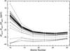 |
Fig. 3 Comparison of our MBPT and MCDHF excitation energies as functions of Z for the lowest 70 singly excited levels. |
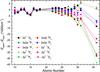 |
Fig. 4 Comparison of our MBPT excitation energies to NIST values (Kramida et al. 2015) as functions of Z for 2l2l′ configurations. |
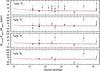
Comparing these wavelengths with the NIST database (Kramida et al. 2015), which contains 197 observed wavelengths, we find that the agreement is within 100 ppm for only 45 transitions. We note, however, that many of these NIST wavelengths are compiled from observations made more than 40 yr ago, which possibly implies large experimental errors. We show the comparison between our MBPT wavelengths and the more recent experimental values in Fig. 2 (in energy units) for 1s21S0−1s2p1P1 (w), 1s2p3P2 (x), 1s2p3P1 (y), 1s2s3S1 (z). In Fig. 5 we also compare our MBPT wavelengths for 1s21S0−1s3p1P1, 1s4p1P1, 1s5p1P1 with the experimental values from the collection of Beiersdorfer et al. (1989) and our MCDHF values. Our MBPT values clearly agree well to within 50 ppm with the experimental values and to within 30 ppm with our MCDHF values.
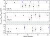 |
Fig. 5 Comparison of our MBPT wavelengths for 1s21S0−1s3p1P1, 1s4p1P1, 1s5p1P1 and the experimental results collected by Beiersdorfer et al. (1989), the differences between our MCDHF and MBPT calculations are also plotted (triangle). |
Figure 6 shows our MBPT wavelengths for all the Δn ≠ 0 E1 transitions of the singly excited levels for some helium-like ions to other theoretical values, including from our own MCDHF calculation, from Savukov et al. (2003), and from Aggarwal et al. (2005, 2009, 2010, 2012d, 2013a). This comparison shows that the agreement between our MBPT and MCDHF values improves with increasing Z, the average differences with standard deviations are −40 ± 108 ppm, −5 ± 48 ppm, 2 ± 28 ppm, 4 ± 20 ppm, 4 ± 14 ppm, 4 ± 13 ppm for Ne IX, Si XIII, Ar XVII, Ti XXI, Fe XXV, and Zn XXIX, respectively. The wavelengths calculated by Savukov et al. (2003) for Ne IX, Si XIII and Ar XVII all agree with our MBPT values to within 500 ppm except for the transitions decaying from 1s6l states. Figure 6 also illustrates that the results of Aggarwal et al.2005 agree less well throughout the sequence, but the case of Ar XVII stands out with a deviation of up to 1% for some 1s5l−1s4l′ transitions.
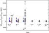 |
Fig. 6 Comparisons of our MBPT wavelengths for Δn ≠ 0 E1 transitions among singly excited levels for Z = 10,14,18,22,26,30 with other theoretical values, i.e., our MCDHF results (bar), values from Savukov et al. (2003; plus) and Aggarwal et al. (2005, 2009, 2010, 2012d, 2013a; cross). As Aggarwal et al. did not provide values for Z = 10, the differences between our MBPT energies and those of Aggarwal et al. for Na IX are plotted instead. |
For the Δn = 0 E1 transition wavelengths of the singly excited levels, the differences between our MBPT and MCDHF values for some 1s5l−1s5l′ and 1s6l−1s6l′ transitions may exceed 1% because of the low transition energies. However, these wavelengths are all longer than 15 000 Å and correspond to very weak transitions. Nonetheless, compared to those from Savukov et al. (2003) and Aggarwal et al. (2005, 2009, 2010, 2012d, 2013a), our MCDHF results agree much better with our MBPT values.
For the wavelengths that decay from doubly excited levels, Goryayev et al. (2006) provided theoretical results for some 2l′2l′′−1s2l and 2l′3l′′−1s2l,1s3l transitions using the Z-expansion method. We compare their results to those from our MBPT calculations in Fig. 7. The differences are generally within 50 ppm except for transitions in the low-Z end. With increasing atomic number, the agreement generally improves when Z ≤ 21, but it deteriorates when Z ≥ 22. The two exceptions are Br XXXIV and Kr XXXV, for which the calculation mode might be changed. The relatively large differences in the low-Z end are mostly likely due to the different treatment of electron correlation effects, while differences in high-Z ions are due to the relativistic effect.
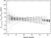 |
Fig. 7 Differences between our MBPT wavelengths and the Z-expansion values provided by Goryayev et al. (2006) for 2l′2l′′−1s2l and 2l′3l′′−1s2l,1s3l transitions. |
3.3. Transition rates
Table 2 also gives our calculated transition rates (A), together with oscillator strengths (f) and line strengths (S). Transition parameters for a transition between two states γPJ and γ′P′J′ can be expressed in terms of reduced matrix elements  where T is the transition operator.
For the transitions presented in Table 2, the NIST database provides rates (line strengths) for 1638 transitions, 787 of them with Z = 10−16 are estimated to be more accurate than 3% (Kramida et al. 2015). Most of these are for resonance E1 transitions. Figure 8 shows that many of them deviate by more than 3% and by up to 18% from our MBPT results, especially for values of Z = 10−14. The reason is probably that the NIST line strength compilation is based on non-relativistic calculations. Figure 8 also shows the differences between the line strengths from our MCDHF and MBPT calculations for these transitions in Ne IX and Si XIII. The two sets of values agree to within 3% for all the corresponding transitions in Ne IX and Si XIII, which confirms the reliability of our MBPT values and indicates that the estimated accuracy in the NIST database might be too optimistic.
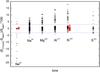 |
Fig. 8 Differences between the NIST line strengths with estimated accuracies lower than 3% (Kramida et al. 2015) and our MBPT values. The differences between our MCDHF and MBPT line strengths (cross) for the corresponding transitions of Ne IX and Si XIII are also plotted. The horizontal lines indicate differences of ±3%. |
Figure 9 shows values for the important resonance E1 transitions from our MBPT calculations for line strengths in Ne IX, Si XIII, Ar XVII, Ti XXI, Fe XXV, and Zn XXIX compared to our MCDHF calculation and that of Savukov et al.2003 and Aggarwal et al. (2005, 2009, 2010, 2012d, 2013a). The average deviations between our MBPT and MCDHF S values are 0.78 ± 3.0%, 0.13 ± 1.0%, 0.09 ± 1.0%, 0.08 ± 0.88%, 0.07 ± 0.67%, and 0.05 ± 0.46% for the presented ions. S values calculated by Savukov et al.2003 also agree well with our MBPT results, with average deviations of 0.77 ± 2.8%, 0.18 ± 0.79%, and 0.16 ± 0.89% for Ne IX, Si XIII, and Ar XVII. Although the differences between our MBPT line strengths and those from Aggarwal et al. (2005, 2009, 2010, 2012d, 2013a) generally decrease with increasing Z (the exception is still Ar XVII), many of the differences in the low-Z end are still larger than 20%.
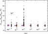 |
Fig. 9 Comparisons of our MBPT S values for resonance E1 transitions among singly excited levels for Z = 10,14,18,22,26,30 with other theoretical values, i.e., our MCDHF results (bar), values from Savukov et al. (2003; plus) and Aggarwal et al. (2005, 2009, 2010, 2012d, 2013a; cross). Since Aggarwal et al. did not provide values for Z = 10, the differences for Z = 11 are plotted instead. |
Table 2 shows that the contributions to radiative lifetimes from non-resonance E1 transitions increase with Z. For the strong non-resonance E1 transitions among singly excited levels that contribute to the total transition rates by more than 0.1%, the average differences between our MBPT and MCDHF results are −8.3 ± 5.5%, −1.8 ± 1.5%, 0.47 ± 1.9%, 0.19 ± 1.3%, 0.07 ± 1.0%, and 0.00 ± 0.70% for Ne IX, Si XIII, Ar XVII, Ti XXI, Fe XXV, and Zn XXIX. Almost all of them agree to within 1% in the high-Z end. Our MBPT line strengths for these strong non-resonance E1 transitions also agree well with those from Savukov et al. (2003), since the differences are −10 ± 4.0%, −3.1 ± 1.5%, and 1.9 ± 5.6% for Ne IX, Si XIII, and Ar XVII.
For transitions that decay from doubly excited levels, we compared our MBPT line strengths with the Z-expansion values from Goryayev et al. (2006). This showed that 78% of the line strengths provided by Goryayev et al. (2006) agree with our MBPT results to within 10%. Larger differences mainly occur in two-electron one-photon (TEOP) transitions, which are more sensitive to electron correlation and relativistic effects. This is illustrated by the example of the line strengths for 2s3s1S0−1s2p1P1 and 2p3s3P0−1s2s3S1 from our MBPT calculation and that of Goryayev et al. (2006) in Fig. 10.
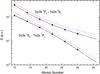 |
Fig. 10 Line strengths for 2s3s1S0−1s2p1P1 and 2p3s3P0−1s2s3S1 as functions of Z from our MBPT (solid line) and tentative MCDHF (triangle) calculations (see text), as well as those from Goryayev et al. (2006; dashed line). |
To substantiate our MBPT line strengths from doubly excited levels, we tentatively calculated doubly excited states using the MCDHF approach. Owing to the convergence problem in the self-consistent procedure, we only included CSFs of the forms nln′l′ (n,n′ ≤ 8,l,l′ ≤ 6). This shows that the two sets of line strengths for strong transitions that contribute to the radiative lifetimes by more than 1% mostly agree to within 10% in the low-Z end and to within 2% in the high-Z end. The complete results from this tentative MCDHF calculation are available from the authors by request. A sample of them is included in Figs. 10 and 11 to support our MBPT results.
3.4. Radiative lifetimes
The radiative lifetime τ for a level j is defined as 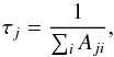 (1)where the sum ∑ iAij runs over all levels lower than level j in energy. Our results for this property are listed in Table 1, which includes the contributions from all possible E1, E2, M1, and M2 radiative decays from levelj. The radiative lifetimes in helium-like ions are almost always dominated by E1 transitions. The only two exceptions are 1s2s3S1 and 1s2p3P2. For the latter, the M2 branching ratio of 1s2p3P2−1s21S0 exceeds the E1 branching ratio 1s2p3P2−1s2s3S1 for Z ≥ 19, and reaches 90% in Kr XXXV. In addition, it should be pointed out that since only single-photon transitions are included in the present work and the 1s2s1S0 state decays mainly by two-photon E1 transitions (Drake 1986), the radiative lifetimes for 1s2s1S0 listed in Table 1 are overestimated by several orders of magnitude.
The two sets of radiative lifetimes for singly excited levels obtained from our MBPT and MCDHF calculations are in excellent agreement, generally agreeing to within 1%. The average differences are 0.21 ± 0.82%, 0.02 ± 0.69%, 0.00 ± 0.82%, 0.05 ± 0.74%, and 0.21 ± 0.51% for Ne IX, Si XIII, Ar XVII, Ti XXI, Fe XXV, and Zn XXIX, respectively. The differences between our MBPT lifetimes and those from Savukov et al. (2003) are generally smaller than 1% as well. However, and as expected, our MBPT results differ substantially from those of Aggarwal et al. (2005, 2008, 2009, 2010, 2011, 2012c,a,d,b, 2013b,a). The largest difference is up to 70% in Na X and still as large as 15% in Kr XXXV.
Our calculations show that the TEOP transitions are crucial in determining the radiative lifetimes of many doubly excited levels. Almost all the radiative lifetimes for levels arising from 2s2 and 2snl′(3 ≤ n ≤ 6) configurations are shortened by more than 50% when TEOP transitions are included. For example, the radiative lifetime of 2s3s3S1 is mainly determined by the 2s3s3S1−1s2p3P1,2,1s3p3P1,2 transitions, which can be seen from Fig. 11a. Additionally, some 2pnl(n> 2) levels such as 2p5s3P2 and 2p5g1F3 are also shortened by more than 10% and up to 60% as a result of the TEOP transitions.
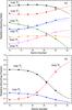 |
Fig. 11 Radiative branching fractions normalized to the total MBPT transition rates of a) 2s3s3S1 and b) 2p3p3D3 as functions of Z from our MBPT (solid line) and tentative MCDHF calculations (scattered symbol, see text), as well as the values from Goryayev et al. (2006; dashed line). |
Furthermore, to determine accurate radiative lifetimes for doubly excited levels, it is not enough to consider radiative channels to singly excited levels, especially for high-Z ions. The lifetimes of many levels arising from 2snl (l ≥ 2) and 2p3d, 2p3p configurations can clearly be shortened by over 10% when transitions between doubly excited states are included. The 2snl (l ≥ 2) configurations thorughout have relatively strong E1 transitions of the form 2snl−2sn′l′ to other doubly excited states, although they can decay to singly excited states through TEOP transitions, as mentioned above. The 2p3d and 2p3p configurations have strong decay channels through 2p3d−2p2 and 2p3p−2s3p. For instance, as shown in Fig. 11b, for the first level with J = 3 and even parity in 2l3l′ configurations (its label turns from 2p3p3D3 to 2s3d3D3 when Z ≥ 20 in Table 1), the main decay channel is to 1s3p3P2 when Z ≤ 26, for Z ≥ 27, the transition to the doubly excited state of 2s2p3P2 becomes the main channel. These strong radiative transitions among the doubly excited levels account for the strong damping effects observed in the resonance excitation for hydrogen-like ions (Li et al. 2015).
The radiative lifetimes for 2l2l′ states obtained from Goryayev et al. (2006) generally agree with our MBPT values to within 10%. However, for about half of the 2l3l′ states, radiative lifetimes from Goryayev et al. (2006) are longer than our MBPT values by over 10% and up to an order of magnitude for many levels. The differences are partly due to the differences in the calculated transition rates, as seen from Fig. 10. More importantly, Goryayev et al. (2006) ignored all the radiative channels between doubly excited states and some important radiative channels to singly excited states, and therefore many of their radiative lifetimes are too long. Figure 11 shows the radiative branching fractions of 2s3s3S1 and 2p3p3D3 (its label turns into 2s3d3D3 when Z ≥ 20) normalized to the total MBPT transition rates as illustrations. The calculated transition rates from Goryayev et al. (2006) agree well with our MBPT values. However, because they neglected several important radiative channels, their radiative lifetimes for 2s3s3S1 are longer than our MBPT values by 50% in Ne IX and a factor of 6 in Kr XXXV, their lifetimes for 2p3p3D3 are longer by 8% for Ne IX and a factor of 30 for Kr XXXV. Finally, it should be pointed out that our MBPT values are verified by our tentative MCDHF results, as presented in Fig. 11.
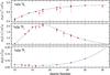 |
Fig. 12 Comparisons of our MBPT (line) and MCDHF (triangle) lifetimes to the experimental values (square) for 1s2s3S1, 1s2p3P2 and 1s2p3P1 states. Experimental data for 1s2s3S1 are taken from Träbert et al. (1999), Stefanelli et al. (1995), Crespo López-Urrutia et al. (2006), Bednar et al. (1975), Hubricht & Träbert (1987), Cocke et al. (1973), and Gould et al. (1974). Values for 1s2p3P2 are adopted from Denne et al. (1980), Deschepper et al. (1982), Cocke et al. (1974b), Cocke et al. (1974a), Dohmann & Mann (1979), Dohmann et al. (1982), Buchet et al. (1984), and Nandi et al. (2004). For 1s2p3P1 the values are taken from Armour et al. (1981) and Varghese et al. (1976). |
To our knowledge, the available measurements of lifetimes for helium-like ions are mostly confined to 1s2l levels (Cocke et al. 1973, 1974a,b; Gould et al. 1974; Bednar et al. 1975; Varghese et al. 1976; Dohmann & Mann 1979; Denne et al. 1980; Armour et al. 1981; Deschepper et al. 1982; Dohmann et al. 1982; Buchet et al. 1984; Hubricht & Träbert 1987; Stefanelli et al. 1995; Träbert et al. 1999; Nandi et al. 2004; Crespo López-Urrutia et al. 2006). Figure 12 shows the comparison of our calculated lifetimes and experimental values as functions of Z for 1s2p3P1, 1s2p3P2 and 1s2s3S1 states. Our MBPT results and the experimental values mostly agree to within the error bars. Our two sets of values also show excellent agreement.
4. Conclusions
We have presented a systematic MBPT calculation of energies and radiative lifetimes among the 1snl(n ≤ 6,l ≤ (n−1)) and 2lnl′(n ≤ 6,l ≤ (n−1)) configurations of helium-like ions with Z = 10−36. Wavelengths, transition rates, oscillator strengths, and line strengths were calculated for all E1, E2, M1, and M2 transitions among these levels. By comparing them to experimental and other theoretical results, the accuracies of our level energies and wavelengths for Δn ≠ 0 transitions are expected to be a few tens of a ppm, the line strengths for strong transitions among singly excited levels and their lifetimes are assessed to be accurate to within 1%, and the precision of the line strengths for strong transitions decaying from doubly excited levels and their radiative lifetimes is better than 10%. Our data are therefore expected to be accurate and comprehensive and will be helpful in line identification, plasma modeling, and diagnostics.
Acknowledgments
This work was supported by NSAF under Grant No. 11076009, National Natural Science Foundation of China under Grant No. 11374062, Chinese Association of Atomic and Molecular Data, and Swedish Research Council 2015-04842. It was also partially supported by the Chinese National Fusion Project for ITER under Grant No. 2015GB117000 and Shanghai Leading Academic Discipline Project under Grant No. B107. R. Si would especially like to acknowledge the International Exchange Program Fund for Doctorate Students of Fudan University Graduate School. One of the authors (KW) expresses his gratitude for the support from the visiting researcher program at Fudan University.
References
- Aggarwal, K. M., & Keenan, F. P. 2005, A&A, 441, 831 [NASA ADS] [CrossRef] [EDP Sciences] [Google Scholar]
- Aggarwal, K. M., & Keenan, F. P. 2008, A&A, 489, 1377 [NASA ADS] [CrossRef] [EDP Sciences] [Google Scholar]
- Aggarwal, K. M., & Keenan, F. P. 2010, Phys. Scr., 82, 065302 [NASA ADS] [CrossRef] [Google Scholar]
- Aggarwal, K. M., & Keenan, F. P. 2012a, Phys. Scr., 85, 025306 [NASA ADS] [CrossRef] [Google Scholar]
- Aggarwal, K. M., & Keenan, F. P. 2012b, Phys. Scr., 86, 035302 [NASA ADS] [CrossRef] [Google Scholar]
- Aggarwal, K. M., & Keenan, F. P. 2012c, Phys. Scr., 85, 025305 [NASA ADS] [CrossRef] [Google Scholar]
- Aggarwal, K. M., & Keenan, F. P. 2012d, Phys. Scr., 85, 065301 [NASA ADS] [CrossRef] [Google Scholar]
- Aggarwal, K. M., & Keenan, F. P. 2013a, Phys. Scr., 87, 055302 [NASA ADS] [CrossRef] [Google Scholar]
- Aggarwal, K. M., & Keenan, F. P. 2013b, Phys. Scr., 87, 045304 [NASA ADS] [CrossRef] [Google Scholar]
- Aggarwal, K. M., Keenan, F. P., & Heeter, R. F. 2009, Phys. Scr., 80, 045301 [NASA ADS] [CrossRef] [Google Scholar]
- Aggarwal, K. M., Kato, T., Keenan, F. P., & Murakami, I. 2011, Phys. Scr., 83, 015302 [NASA ADS] [CrossRef] [Google Scholar]
- Amaro, P., Schlesser, S., Guerra, M., et al. 2012, Phys. Rev. Lett., 109, 043005 [NASA ADS] [CrossRef] [PubMed] [Google Scholar]
- Armour, I. A., Silver, J. D., & Trabert, E. 1981, J. Phys. B, 14, 3563 [NASA ADS] [CrossRef] [Google Scholar]
- Artemyev, A. N., Shabaev, V. M., Yerokhin, V. A., Plunien, G., & Soff, G. 2005, Phys. Rev. A, 71, 062104 [NASA ADS] [CrossRef] [Google Scholar]
- Bednar, J. A., Cocke, C. L., Curnutte, B., & Randall, R. 1975, Phys. Rev. A, 11, 460 [NASA ADS] [CrossRef] [Google Scholar]
- Beiersdorfer, P. 2015, J. Phys. B, 48, 144017 [NASA ADS] [CrossRef] [Google Scholar]
- Beiersdorfer, P., Bitter, M., von Goeler, S., & Hill, K. W. 1989, Phys. Rev. A, 40, 150 [NASA ADS] [CrossRef] [Google Scholar]
- Beiersdorfer, P., & Brown, G. V. 2015, Phys. Rev. A, 91, 032514 [NASA ADS] [CrossRef] [Google Scholar]
- Beiersdorfer, P., Osterheld, A. L., Phillips, T. W., et al. 1995, Phys. Rev. E, 52, 1980 [NASA ADS] [CrossRef] [Google Scholar]
- Bombarda, F., Giannella, R., Källne, E., et al. 1988, Phys. Rev. A, 37, 504 [NASA ADS] [CrossRef] [PubMed] [Google Scholar]
- Briand, J. P., Mossé, J. P., Indelicato, P., et al. 1983, Phys. Rev. A, 28, 1413 [NASA ADS] [CrossRef] [Google Scholar]
- Bruhns, H., Braun, J., Kubiček, K., Crespo López-Urrutia, J. R., & Ullrich, J. 2007, Phys. Rev. Lett., 99, 113001 [NASA ADS] [CrossRef] [PubMed] [Google Scholar]
- Buchet, J. P., Buchet-Poulizac, M. C., Denis, A., et al. 1984, Phys. Rev. A, 30, 309 [NASA ADS] [CrossRef] [Google Scholar]
- Bucksbaum, P. H., Coffee, R., & Berrah, N. 2011, in Advances In Atomic, Molecular, and Optical Physics, eds. P. B. E. Arimondo, & C. Lin (Elsevier), 60, 239 [Google Scholar]
- Chantler, C. T., Paterson, D., Hudson, L. T., et al. 2000, Phys. Rev. A, 62, 042501 [NASA ADS] [CrossRef] [Google Scholar]
- Chantler, C. T., Kinnane, M. N., Gillaspy, J. D., et al. 2012, Phys. Rev. Lett., 109, 153001 [NASA ADS] [CrossRef] [Google Scholar]
- Chen, M. H., Cheng, K. T., & Johnson, W. R. 1993, Phys. Rev. A, 47, 3692 [NASA ADS] [CrossRef] [Google Scholar]
- Cheng, K. T., & Chen, M. H. 2000, Phys. Rev. A, 61, 044503 [NASA ADS] [CrossRef] [Google Scholar]
- Cheng, K. T., Chen, M. H., Johnson, W. R., & Sapirstein, J. 1994, Phys. Rev. A, 50, 247 [NASA ADS] [CrossRef] [PubMed] [Google Scholar]
- Cocke, C. L., Curnutte, B., & Randall, R. 1973, Phys. Rev. Lett., 31, 507 [NASA ADS] [CrossRef] [Google Scholar]
- Cocke, C. L., Curnutte, B., Macdonald, J. R., & Randall, R. 1974a, Phys. Rev. A, 9, 57 [NASA ADS] [CrossRef] [Google Scholar]
- Cocke, C. L., Curnutte, B., & Randall, R. 1974b, Phys. Rev. A, 9, 1823 [NASA ADS] [CrossRef] [Google Scholar]
- Cornille, M., Dubau, J., Bely-Dubau, F., et al. 1990, J. Phys. B, 23, 4451 [NASA ADS] [CrossRef] [Google Scholar]
- Crespo López-Urrutia, J. R., Beiersdorfer, P., & Widmann, K. 2006, Phys. Rev. A, 74, 012507 [NASA ADS] [CrossRef] [Google Scholar]
- Deng-Hong, Z., Chen-Zhong, D., & Koike, F. 2006, Chin. Phys. Lett., 23, 2059 [NASA ADS] [CrossRef] [Google Scholar]
- Denne, B., Huldt, S., Pihl, J., & Hallin, R. 1980, Phys. Scr., 22, 45 [NASA ADS] [CrossRef] [Google Scholar]
- Dere, K. P., Landi, E., Young, P. R., & Zanna, G. D. 2001, ApJS, 134, 331 [NASA ADS] [CrossRef] [Google Scholar]
- Deschepper, P., Lebrun, P., Palffy, L., & Pellegrin, P. 1982, Phys. Rev. A, 26, 1271 [NASA ADS] [CrossRef] [Google Scholar]
- Deslattes, R. D., Beyer, H. F., & Folkmann, F. 1984, J. Phys. B, 17, L689 [NASA ADS] [CrossRef] [Google Scholar]
- Dohmann, H., & Mann, R. 1979, Z. Phys. A, 15, 22 [Google Scholar]
- Dohmann, H., Mann, R., & Pfeng, E. 1982, Z. Phys. A, 309, 101 [Google Scholar]
- Doyle, J. G., & Keenan, F. P. 1986, A&A, 157, 116 [NASA ADS] [Google Scholar]
- Drake, G. W. 1988, Can. J. Phys., 66, 586 [NASA ADS] [CrossRef] [Google Scholar]
- Drake, G. W. F. 1986, Phys. Rev. A, 34, 2871 [NASA ADS] [CrossRef] [PubMed] [Google Scholar]
- Dubau, J., Gabriel, A. H., Loulergue, M., Steenman-Clark, L., & Volonté, S. 1981, MNRAS, 195, 705 [NASA ADS] [CrossRef] [Google Scholar]
- Düsterer, S., Radcliffe, P., Bostedt, C., et al. 2011, New J. Phys., 13, 093024 [NASA ADS] [CrossRef] [Google Scholar]
- Dyall, K., Grant, I., Johnson, C., Parpia, F., & Plummer, E. 1989, Comput. Phys. Commun., 55, 425 [NASA ADS] [CrossRef] [Google Scholar]
- Elton, R., Cobble, J., Griem, H., et al. 2000, J. Quant. Spec. Radiat. Transf., 65, 185 [NASA ADS] [CrossRef] [Google Scholar]
- Epp, S. W., Steinbrügge, R., Bernitt, S., et al. 2015, Phys. Rev. A, 92, 020502 [NASA ADS] [CrossRef] [Google Scholar]
- Fei, Z., Li, W., Grumer, J., et al. 2014, Phys. Rev. A, 90, 052517 [NASA ADS] [CrossRef] [Google Scholar]
- Feldman, U., Curdt, W., Landi, E., & Wilhelm, K. 2000, ApJ, 544, 508 [NASA ADS] [CrossRef] [Google Scholar]
- Gabriel, A. H. 1972, MNRAS, 160, 99 [NASA ADS] [Google Scholar]
- Gabriel, A. H., & Jordan, C. 1969, MNRAS, 145, 241 [NASA ADS] [CrossRef] [Google Scholar]
- Gabriel, A. H., & Jordan, C. 1969, Nature, 221, 947 [NASA ADS] [CrossRef] [Google Scholar]
- Goryayev, F. F., Urnov, A. M., & Vainshtein, L. A. 2006, ArXiv e-prints [arXiv:physics/0603164] [Google Scholar]
- Gould, H., Marrus, R., & Mohr, P. J. 1974, Phys. Rev. Lett., 33, 676 [NASA ADS] [CrossRef] [Google Scholar]
- Grant, I., McKenzie, B., Norrington, P., Mayers, D., & Pyper, N. 1980, Comput. Phys. Commun., 21, 207 [NASA ADS] [CrossRef] [Google Scholar]
- Gu, M. F. 2005, ApJS, 156, 105 [NASA ADS] [CrossRef] [Google Scholar]
- Gu, M. F. 2007, ApJS, 169, 154 [NASA ADS] [CrossRef] [Google Scholar]
- Gu, M. F. 2008, Can. J. Phys., 86, 675 [NASA ADS] [CrossRef] [Google Scholar]
- Gu, M. F., Holczer, T., Behar, E., & Kahn, S. M. 2006, ApJ, 641, 1227 [NASA ADS] [CrossRef] [Google Scholar]
- Gu, M. F., Beiersdorfer, P., & Lepson, J. K. 2011, ApJ, 732, 91 [NASA ADS] [CrossRef] [Google Scholar]
- Güdel, M., & Nazé, Y. 2009, A&ARv, 17, 309 [NASA ADS] [CrossRef] [Google Scholar]
- Guo, X. L., Huang, M., Yan, J., et al. 2015, J. Phys. B, 48, 144020 [NASA ADS] [CrossRef] [Google Scholar]
- Harra-Murnion, L. K., Phillips, K. J. H., Lemen, J. R., et al. 1996, A&A, 308, 670 [NASA ADS] [Google Scholar]
- Hsuan, H., Bitter, M., Hill, K. W., et al. 1987, Phys. Rev. A, 35, 4280 [NASA ADS] [CrossRef] [Google Scholar]
- Hubricht, G., & Träbert, E. 1987, Z. Phys. D, 7, 243 [Google Scholar]
- Indelicato, P., Briand, J., Tavernier, M., & Liesen, D. 1986, Z. Phys. D, 2, 249 [Google Scholar]
- Johnson, W., Plante, D., & Sapirstein, J. 1995, Adv. At., Mol. Opt. Phys., 35, 255 [Google Scholar]
- Johnson, W. R., Savukov, I. M., Safronova, U. I., & Dalgarno, A. 2002, ApJS, 141, 543 [NASA ADS] [CrossRef] [Google Scholar]
- Jönsson, P., Gaigalas, G., Bieroń, J., Fischer, C. F., & Grant, I. 2013, Comput. Phys. Commun., 184, 2197 [NASA ADS] [CrossRef] [Google Scholar]
- Kadrekar, R., & Natarajan, L. 2011, Phys. Rev. A, 84, 062506 [NASA ADS] [CrossRef] [Google Scholar]
- Kallman, T. R., & Palmeri, P. 2007, Rev. Mod. Phys., 79, 79 [NASA ADS] [CrossRef] [Google Scholar]
- Källne, E., Källne, J., & Pradhan, A. K. 1983, Phys. Rev. A, 27, 1476 [NASA ADS] [CrossRef] [Google Scholar]
- Kanter, E. P., Krässig, B., Li, Y., et al. 2011, Phys. Rev. Lett., 107, 233001 [NASA ADS] [CrossRef] [PubMed] [Google Scholar]
- Karim, K. 2010, J. Quant. Spec. Radiat. Transf., 111, 384 [NASA ADS] [CrossRef] [Google Scholar]
- Karim, K. R., & Bhalla, C. P. 1986, Phys. Rev. A, 34, 4743 [NASA ADS] [CrossRef] [Google Scholar]
- Karim, K. R., & Bhalla, C. P. 1995, J. Phys. B, 28, 5229 [NASA ADS] [CrossRef] [Google Scholar]
- Karim, K. R., Ruesink, M., & Bhalla, C. P. 1992, Phys. Rev. A, 46, 3904 [NASA ADS] [CrossRef] [Google Scholar]
- Kasthurirangan, S., Saha, J. K., Agnihotri, A. N., et al. 2013, Phys. Rev. Lett., 111, 243201 [NASA ADS] [CrossRef] [Google Scholar]
- Keenan, F. P., Tayal, S. S., & Kingston, A. E. 1984, Sol. Phys., 94, 85 [NASA ADS] [CrossRef] [Google Scholar]
- Keenan, F. P., McCann, S. M., Barnsley, R., et al. 1989, Phys. Rev. A, 39, 4092 [NASA ADS] [CrossRef] [Google Scholar]
- Kharchenko, V., & Dalgarno, A. 2001, ApJ, 554, L99 [NASA ADS] [CrossRef] [Google Scholar]
- Kramida, A., Yu. Ralchenko, Reader, J., & and NIST ASD Team. 2015, NIST Atomic Spectra Database (ver. 5.2), [Online]. Available: http://physics.nist.gov/asd [2015, October 6]. National Institute of Standards and Technology, Gaithersburg, MD [Google Scholar]
- Kubiček, K., Bruhns, H., Braun, J., López-Urrutia, J. R. C., & Ullrich, J. 2009, J. Phys. Conf. Ser., 163, 012007 [NASA ADS] [CrossRef] [Google Scholar]
- Kubiček, K., Mokler, P. H., Ullrich, J., & López-Urrutia, J. R. C. 2013, Phys. Scr., 2013, 014005 [Google Scholar]
- Landi, E., & Phillips, K. J. H. 2005, ApJS, 160, 286 [NASA ADS] [CrossRef] [Google Scholar]
- Li, S., Yan, J., Li, C. Y., et al. 2015, A&A, 583, A82 [NASA ADS] [CrossRef] [EDP Sciences] [Google Scholar]
- Lindgren, I. 1974, J. Phys. B, 7, 2441 [NASA ADS] [CrossRef] [Google Scholar]
- MacLaren, S., Beiersdorfer, P., Vogel, D. A., et al. 1992, Phys. Rev. A, 45, 329 [NASA ADS] [CrossRef] [Google Scholar]
- Martin, W. C., & Zalubas, R. 1981, J. Phys. Chem. Ref. Data, 10, 153 [NASA ADS] [CrossRef] [Google Scholar]
- Martin, W. C., & Zalubas, R. 1983, J. Phys. Chem. Ref. Data, 12, 323 [NASA ADS] [CrossRef] [Google Scholar]
- Martin, W. C., Zalubas, R., & Musgrove, A. 1985, J. Phys. Chem. Ref. Data, 14, 751 [NASA ADS] [CrossRef] [Google Scholar]
- McKenzie, D. L., Broussard, R. M., Landecker, P. B., et al. 1979, in BAAS, 11, 676 [Google Scholar]
- McKenzie, B., Grant, I., & Norrington, P. 1980, Comput. Phys. Commun., 21, 233 [NASA ADS] [CrossRef] [Google Scholar]
- Meyer, M., Radcliffe, P., Tschentscher, T., et al. 2012, Phys. Rev. Lett., 108, 063007 [NASA ADS] [CrossRef] [PubMed] [Google Scholar]
- Mosnier, J. P., Barchewitz, R., Cukier, M., et al. 1986, J. Phys. B, 19, 2531 [NASA ADS] [CrossRef] [Google Scholar]
- Nakano, Y., Suda, S., Hatakeyama, A., et al. 2012, Phys. Rev. A, 85, 020701 [NASA ADS] [CrossRef] [Google Scholar]
- Nandi, T. 2008, ApJ, 673, L103 [NASA ADS] [CrossRef] [Google Scholar]
- Nandi, T., Wani, A. A., Ahmad, N., et al. 2004, J. Phys. B, 37, 703 [NASA ADS] [CrossRef] [Google Scholar]
- Natarajan, L. 2014, Phys. Rev. A, 90, 032509 [NASA ADS] [CrossRef] [Google Scholar]
- Natarajan, L., & Kadrekar, R. 2013, Phys. Rev. A, 88, 012501 [NASA ADS] [CrossRef] [Google Scholar]
- Ness, J.-U., Brickhouse, N. S., Drake, J. J., & Huenemoerder, D. P. 2003, ApJ, 598, 1277 [NASA ADS] [CrossRef] [Google Scholar]
- O’Rourke, B. E., Currell, F. J., Kuramoto, H., et al. 2008, Phys. Rev. A, 77, 062709 [NASA ADS] [CrossRef] [Google Scholar]
- Paerels, F. B. S., & Kahn, S. M. 2003, ARA&A, 41, 291 [NASA ADS] [CrossRef] [Google Scholar]
- Parmar, A. N., Culhane, J. L., Rapley, C. G., et al. 1981, MNRAS, 197, 29P [NASA ADS] [CrossRef] [Google Scholar]
- Parpia, F. A., Tong, M., & Fischer, C. F. 1992, Phys. Rev. A, 46, 3717 [NASA ADS] [CrossRef] [PubMed] [Google Scholar]
- Payne, A. T., Chantler, C. T., Kinnane, M. N., et al. 2014, J. Phys. B, 47, 185001 [NASA ADS] [CrossRef] [Google Scholar]
- Phillips, K. J. H. 2004, ApJ, 605, 921 [NASA ADS] [CrossRef] [Google Scholar]
- Phillips, K. J. H., Harra, L. K., Keenan, F. P., Zarro, D. M., & Wilson, M. 1993, ApJ, 419, 426 [NASA ADS] [CrossRef] [Google Scholar]
- Pike, C. D., Phillips, K. J. H., Lang, J., et al. 1996, ApJ, 464, 487 [NASA ADS] [CrossRef] [Google Scholar]
- Plante, D. R., Johnson, W. R., & Sapirstein, J. 1994, Phys. Rev. A, 49, 3519 [NASA ADS] [CrossRef] [PubMed] [Google Scholar]
- Porquet, D., Mewe, R., Dubau, J., Raassen, A. J. J., & Kaastra, J. S. 2001, A&A, 376, 1113 [NASA ADS] [CrossRef] [EDP Sciences] [Google Scholar]
- Porquet, D., Dubau, J., & Grosso, N. 2010, Space Sci. Rev., 157, 103 [NASA ADS] [CrossRef] [Google Scholar]
- Pradhan, A. K., & Shull, J. M. 1981, ApJ, 249, 821 [NASA ADS] [CrossRef] [Google Scholar]
- Rice, J. E., Marmar, E. S., Källne, E., & Källne, J. 1987, Phys. Rev. A, 35, 3033 [NASA ADS] [CrossRef] [Google Scholar]
- Rice, J. E., Fournier, K. B., Safronova, U. I., et al. 1999, New J. Phys., 1, 19 [NASA ADS] [CrossRef] [Google Scholar]
- Rice, J. E., Goetz, J. A., Granetz, R. S., et al. 2000, Phys. Plasmas, 7, 1825 [NASA ADS] [CrossRef] [Google Scholar]
- Rice, J. E., Reinke, M. L., Ashbourn, J. M. A., et al. 2014, J. Phys. B, 47, 075701 [NASA ADS] [CrossRef] [Google Scholar]
- Rice, J. E., Reinke, M. L., Ashbourn, J. M. A., et al. 2015, J. Phys. B, 48, 144013 [NASA ADS] [CrossRef] [Google Scholar]
- Rosmej, F. B., Griem, H. R., Elton, R. C., et al. 2002, Phys. Rev. E, 66, 056402 [NASA ADS] [CrossRef] [Google Scholar]
- Rudolph, J. K., Bernitt, S., Epp, S. W., et al. 2013, Phys. Rev. Lett., 111, 103002 [NASA ADS] [CrossRef] [Google Scholar]
- Safronova, M. S., Johnson, W. R., & Safronova, U. I. 1996, Phys. Rev. A, 53, 4036 [NASA ADS] [CrossRef] [Google Scholar]
- Safronova, U. I., & Senashenko, V. S. 1977, J. Phys. B, 10, L271 [NASA ADS] [CrossRef] [Google Scholar]
- Saloman, E. B. 2010, J. Phys. Chem. Ref. Data, 39, 033101 [NASA ADS] [CrossRef] [Google Scholar]
- Savukov, I., Johnson, W., & Safronova, U. 2003, At. Data Nucl. Data Tables, 85, 83 [Google Scholar]
- Schleinkofer, L., Bell, F., Betz, H.-D., Trollmann, G., & Rothermel, J. 1982, Phys. Scr., 25, 917 [NASA ADS] [CrossRef] [Google Scholar]
- Schlesser, S., Boucard, S., Covita, D. S., et al. 2013, Phys. Rev. A, 88, 022503 [NASA ADS] [CrossRef] [Google Scholar]
- Seely, J. F., & Feldman, U. 1985, Phys. Rev. Lett., 54, 1016 [NASA ADS] [CrossRef] [Google Scholar]
- Si, R., Guo, X., Yan, J., et al. 2015a, J. Quant. Spec. Radiat. Transf., 163, 7 [NASA ADS] [CrossRef] [Google Scholar]
- Si, R., Guo, X. L., Yan, J., et al. 2015b, J. Phys. B, 48, 175004 [Google Scholar]
- Smith, R. K. 2014, in Amer. Astron. Soc. Meet. Abstracts, 224, 106.01 [Google Scholar]
- Smith, R. K., Brickhouse, N. S., Liedahl, D. A., & Raymond, J. C. 2001, ApJ, 556, L91 [NASA ADS] [CrossRef] [Google Scholar]
- Stefanelli, G. S., Beiersdorfer, P., Decaux, V., & Widmann, K. 1995, Phys. Rev. A, 52, 3651 [NASA ADS] [CrossRef] [PubMed] [Google Scholar]
- Sucher, J. 1980, Phys. Rev. A, 22, 348 [NASA ADS] [CrossRef] [MathSciNet] [Google Scholar]
- Sylwester, J., Sylwester, B., Phillips, K. J. H., & Kuznetsov, V. D. 2010, ApJ, 710, 804 [NASA ADS] [CrossRef] [Google Scholar]
- Tanaka, K. 1986, PASJ, 38, 225 [NASA ADS] [Google Scholar]
- Träbert, E., Beiersdorfer, P., Brown, G. V., et al. 1999, Phys. Rev. A, 60, 2034 [NASA ADS] [CrossRef] [Google Scholar]
- Vainshtein, L., & Safronova, U. 1978, At. Data Nucl. Data Tables, 21, 49 [Google Scholar]
- Vainshtein, L., & Safronova, U. 1980, At. Data Nucl. Data Tables, 25, 311 [Google Scholar]
- Vainshtein, L. A., & Safronova, U. I. 1976, P. N. Lebedev Phys. Inst., Acad. Sci. USSR, Moscow., 146 [Google Scholar]
- Vainshtein, L. A., & Safronova, U. I. 1985, Acad. Nauk. USSR, Inst. Spectrosc., Moscow [Google Scholar]
- Varghese, S. L., Cocke, C. L., & Curnutte, B. 1976, Phys. Rev. A, 14, 1729 [NASA ADS] [CrossRef] [Google Scholar]
- Walker, Jr., A. B. C., & Rugge, H. R. 1970, A&A, 5, 4 [NASA ADS] [Google Scholar]
- Wang, K., Li, D. F., Liu, H. T., et al. 2014, ApJS, 215, 26 [NASA ADS] [CrossRef] [Google Scholar]
- Wang, K., Guo, X. L., Liu, H. T., et al. 2015, ApJS, 218, 16 [NASA ADS] [CrossRef] [Google Scholar]
- Widmann, K., Beiersdorfer, P., Decaux, V., & Bitter, M. 1996, Phys. Rev. A, 53, 2200 [NASA ADS] [CrossRef] [Google Scholar]
- Wolfson, C. J., Leibacher, J. W., Doyle, J. G., & Phillips, K. J. H. 1983, ApJ, 269, 319 [NASA ADS] [CrossRef] [Google Scholar]
- Yamamoto, N., Kato, T., & Rosmej, F. B. 2005, J. Quant. Spec. Radiat. Transf., 96, 343 [NASA ADS] [CrossRef] [Google Scholar]
- Young, L., Kanter, E. P., Krässig, B., et al. 2010, Nature, 466, 56 [NASA ADS] [CrossRef] [PubMed] [Google Scholar]
All Tables
Level designations, excitation energies (in cm-1), and lifetimes (τ in s) for the 321 levels arising from the 1snl(n ≤ 6,l ≤ (n−1)) and 2ln′l′(n′ ≤ 6,l′ ≤ (n′−1)) configurations of helium-like ions with Z = 10−36.
Wavelengths (λ, in Å), transition rates (A, in s-1), oscillator strengths (f, dimensionless), and line strengths (S, in a.u.) for transitions among 1snl(n ≤ 6,l ≤ (n−1)) and 2ln′l′(n′ ≤ 6,l′ ≤ (n′−1)) configurations in helium-like ions with Z = 10−36.
All Figures
|
Fig. 1 Comparison of our MBPT energies to NIST values (Kramida et al. 2015) as a function of Z for 1s2l configurations. The horizontal lines indicate differences of ±1000 cm-1. |
| In the text | |
|
Fig. 3 Comparison of our MBPT and MCDHF excitation energies as functions of Z for the lowest 70 singly excited levels. |
| In the text | |
|
Fig. 4 Comparison of our MBPT excitation energies to NIST values (Kramida et al. 2015) as functions of Z for 2l2l′ configurations. |
| In the text | |
|
Fig. 5 Comparison of our MBPT wavelengths for 1s21S0−1s3p1P1, 1s4p1P1, 1s5p1P1 and the experimental results collected by Beiersdorfer et al. (1989), the differences between our MCDHF and MBPT calculations are also plotted (triangle). |
| In the text | |
|
Fig. 6 Comparisons of our MBPT wavelengths for Δn ≠ 0 E1 transitions among singly excited levels for Z = 10,14,18,22,26,30 with other theoretical values, i.e., our MCDHF results (bar), values from Savukov et al. (2003; plus) and Aggarwal et al. (2005, 2009, 2010, 2012d, 2013a; cross). As Aggarwal et al. did not provide values for Z = 10, the differences between our MBPT energies and those of Aggarwal et al. for Na IX are plotted instead. |
| In the text | |
|
Fig. 7 Differences between our MBPT wavelengths and the Z-expansion values provided by Goryayev et al. (2006) for 2l′2l′′−1s2l and 2l′3l′′−1s2l,1s3l transitions. |
| In the text | |
|
Fig. 8 Differences between the NIST line strengths with estimated accuracies lower than 3% (Kramida et al. 2015) and our MBPT values. The differences between our MCDHF and MBPT line strengths (cross) for the corresponding transitions of Ne IX and Si XIII are also plotted. The horizontal lines indicate differences of ±3%. |
| In the text | |
|
Fig. 9 Comparisons of our MBPT S values for resonance E1 transitions among singly excited levels for Z = 10,14,18,22,26,30 with other theoretical values, i.e., our MCDHF results (bar), values from Savukov et al. (2003; plus) and Aggarwal et al. (2005, 2009, 2010, 2012d, 2013a; cross). Since Aggarwal et al. did not provide values for Z = 10, the differences for Z = 11 are plotted instead. |
| In the text | |
|
Fig. 10 Line strengths for 2s3s1S0−1s2p1P1 and 2p3s3P0−1s2s3S1 as functions of Z from our MBPT (solid line) and tentative MCDHF (triangle) calculations (see text), as well as those from Goryayev et al. (2006; dashed line). |
| In the text | |
|
Fig. 11 Radiative branching fractions normalized to the total MBPT transition rates of a) 2s3s3S1 and b) 2p3p3D3 as functions of Z from our MBPT (solid line) and tentative MCDHF calculations (scattered symbol, see text), as well as the values from Goryayev et al. (2006; dashed line). |
| In the text | |
|
Fig. 12 Comparisons of our MBPT (line) and MCDHF (triangle) lifetimes to the experimental values (square) for 1s2s3S1, 1s2p3P2 and 1s2p3P1 states. Experimental data for 1s2s3S1 are taken from Träbert et al. (1999), Stefanelli et al. (1995), Crespo López-Urrutia et al. (2006), Bednar et al. (1975), Hubricht & Träbert (1987), Cocke et al. (1973), and Gould et al. (1974). Values for 1s2p3P2 are adopted from Denne et al. (1980), Deschepper et al. (1982), Cocke et al. (1974b), Cocke et al. (1974a), Dohmann & Mann (1979), Dohmann et al. (1982), Buchet et al. (1984), and Nandi et al. (2004). For 1s2p3P1 the values are taken from Armour et al. (1981) and Varghese et al. (1976). |
| In the text | |
Current usage metrics show cumulative count of Article Views (full-text article views including HTML views, PDF and ePub downloads, according to the available data) and Abstracts Views on Vision4Press platform.
Data correspond to usage on the plateform after 2015. The current usage metrics is available 48-96 hours after online publication and is updated daily on week days.
Initial download of the metrics may take a while.