© ESO, 2016

1. Introduction

Supernova (SN) data have provided evidence that distant sources (z> 0.3) appear dimmer than predicted in a universe with matter only, in comparison with nearby sources. This dimming led to the interpretation that the Universe is expanding in an accelerating fashion. This acceleration has been attributed to a dark energy component, whose simplest solution is a vacuum energy or equivalently a cosmological constant. However, this dimming could be caused by a variation of any other component that affects the luminosity distance, namely by inhomogeneities in the energy densities or in the cosmic expansion (Amendola et al. 2013).

In order to explain the underlying mechanism of the late-time accelerated expansion of the universe, one possibility is to give up of the cosmological principle and allow for an anisotropic expansion of the universe. The idea that we live in a locally underdense region, hence creating a “Hubble bubble”, can explain the cosmic acceleration at late times, subject to specific conditions (Zehavi et al. 1998; Caldwell & Stebbins 2008). From the vast literature on the cosmological principle, it has been found that most cosmological observations can accommodate violations of the cosmological principle (see for example Zibin et al. 2008; Tomita & Inoue 2009; Marra & Pääkkönen 2010; Marra & Notari 2011; Moss et al. 2011). From the theoretical point of view, violations of the cosmological principle can be explained in the context of Lemaître-Tolman-Bondi (LTB) void models. These void models are spherically symmetric and radially inhomogeneous, and can mimic the cosmic expansion of the concordance ΛCDM (Lan et al. 2010; Liu & Zhang 2014).

In Carvalho & Marques (2016), we introduced a method to probe the inhomogeneity of the large-scale structure by measuring the angular distribution in the cosmological parameters that affect the luminosity distance, using SN data. Variation in the cosmological parameters across pixels in the sky implies inhomogeneity in the cosmic expansion. This inhomogeneity was then used to measure the extra component of cosmic acceleration predicted by backreaction, which derives from averaging over an inhomogeneous ensemble of homogeneous pixels, each pixel expanding at a different rate. However, this measurement presupposed an a priori dark energy component in each pixel. In order to investigate alternative interpretations of the cosmic acceleration, it is conceptually more consistent to use a parametrisation that does not assume a specific component as the cause of acceleration (Turner & Riess 2002).

In this manuscript, we use the luminosity distance expressed in terms of time derivatives of the scale factor a(z), in particular the Hubble parameter H₀, the deceleration parameter q₀ and the jerk parameter j₀. Instead of assuming an equation of state and inferring the evolution of the scale factor via the Friedmann equation, the reasoning is to take the data on the scale factor and infer a cosmological equation of state via the Friedmann equation. This parametrisation records the cosmic expansion without regard to its cause, thus being independent of the cosmological equation of state adequate to test interpretations of the cosmic acceleration alternative to the cosmological constant. These parameters can be related to the Taylor expansion of the cosmological equation of state about the present values { ρ₀,p₀ } expressed up to linear order as $\begin{array}{ccc}\mathit{p}\mathrm{=}{\mathit{p}}_{\mathrm{0}}\mathrm{+}{\mathit{\kappa }}_{\mathrm{0}}\mathrm{(}\mathit{\rho }\mathrm{-}{\mathit{\rho }}_{\mathrm{0}}\mathrm{)}\mathrm{+}\mathit{O}\mathrm{[}\mathrm{(}\mathit{\rho }\mathrm{-}{\mathit{\rho }}_{\mathrm{0}}{\mathrm{)}}^{\mathrm{2}}\mathrm{]}\mathit{,}& & \end{array}$(1)hence yielding information about the present values of w₀ and κ₀ defined as (Visser 2004) $\begin{array}{ccc}{\mathit{w}}_{\mathrm{0}}\mathrm{=}\frac{\mathit{p}}{\mathit{\rho }}{|}_{\mathrm{0}}\mathrm{\equiv }{\mathit{w}}_{\mathrm{0}}\mathrm{\left(}{\mathit{H}}_{\mathrm{0}}\mathit{,}{\mathit{q}}_{\mathrm{0}}\mathrm{\right)}\mathit{,} {\mathit{\kappa }}_{\mathrm{0}}\mathrm{=}\frac{\mathrm{d}\mathit{p}}{\mathrm{d}\mathit{\rho }}{|}_{\mathrm{0}}\mathrm{\equiv }{\mathit{\kappa }}_{\mathrm{0}}\mathrm{\left(}{\mathit{H}}_{\mathrm{0}}\mathit{,}{\mathit{q}}_{\mathrm{0}}\mathit{,}{\mathit{j}}_{\mathrm{0}}\mathrm{\right)}\mathit{.}& & \end{array}$(2)Whereas w₀ (and hence q₀) contains information about the present value of p/ρ,κ₀ (and hence j₀) contains information about how w₀ can evolve.

The purpose of this manuscript is to reapply the method first presented in Carvalho & Marques (2016) to estimate the parameters { H₀,q₀,j₀ } , instead of { H₀,Ω_M,Ω_Λ } , by fitting the luminosity distance to SN data, and to compare the results from the two estimations in view of an interpretation of the cosmic acceleration independent of a particular energy content of the Universe. (Although the comparisons are made for the case that Ω_κ = 1−Ω_M−Ω_Λ, for completion we also include the results for the case where Ω_κ = 0.) Some studies have used the kinematic parametrization to measure inhomogeneities from SN data (see e.g. Schwarz & Weinhorst 2007; Kalus et al. 2013). Most studies, however, have aimed at finding hemispherical anisotropies assuming a ΛCDM energy content (e.g. Blomqvist et al. 2010; Mariano & Perivolaropoulos 2012; Heneka et al. 2014; Jiménez et al. 2015; Bengaly et al. 2015a; Javanmardi et al. 2015; Migkas & Plionis 2016 and references therein).

This paper is organised as follows. In Sect. 2 we describe the data and estimate the observables by performing both a global and a local parameter estimation, obtaining fiducial values and maps respectively for the estimated parameters. We introduce an inhomogeneity test by rotating the supernova subsampling per pixel. In Sect. 3 we compute the power spectrum of the maps of the parameters using two methods for the noise bias removal. In Sect. 4, for the same toy model of backreaction used in Carvalho & Marques (2016), we compute the average values of { q₀,j₀ } and discuss possible cosmological implications. In Sect. 5 we draw conclusions.

2. Parameter estimation

We use the type Ia supernova sample compiled by the Joint Light-curve Analysis (JLA) collaborative effort (Betoule et al. 2014) from different supernova surveys, totalling N_SNe = 740 supernovae (SNe) with redshift z ∈ [0.010,1.30] and distributed on the sky according to Fig. 1 in Carvalho & Marques (2016)¹.

We use the luminosity distance d_L with a(z) expressed as a Taylor expansion about the present value a(z₀) (Visser 2004) $\begin{array}{ccc}& & {\mathit{d}}_{\mathrm{L}}\mathrm{\left(}\mathit{z}\mathrm{;}{\mathit{H}}_{\mathrm{0}}\mathit{,}{\mathit{q}}_{\mathrm{0}}\mathit{,}{\mathit{j}}_{\mathrm{0}}\mathrm{\right)}\mathrm{=}\frac{\mathit{cz}}{{\mathit{H}}_{\mathrm{0}}}\\ & & \mathrm{\times }\hspace{0.17em}\hspace{0.17em}[\mathrm{1}\mathrm{+}\frac{\mathrm{1}}{\mathrm{2}}\mathrm{(}\mathrm{1}\mathrm{-}{\mathit{q}}_{\mathrm{0}}\mathrm{)}\mathit{z}\mathrm{-}\frac{\mathrm{1}}{\mathrm{6}}\left(\mathrm{1}\mathrm{-}{\mathit{q}}_{\mathrm{0}}\mathrm{-}\mathrm{3}{\mathit{q}}_{\mathrm{0}}^{\mathrm{2}}\mathrm{+}{\mathit{j}}_{\mathrm{0}}\mathrm{+}\frac{\mathit{k}{\mathit{c}}^{\mathrm{2}}}{{\mathit{H}}_{\mathrm{0}}^{\mathrm{2}}{\mathit{a}}_{\mathrm{0}}^{\mathrm{2}}}\right){\mathit{z}}^{\mathrm{2}}\\ & & \end{array}$(3)to estimate the cosmological parameters that minimise the chi-square of the fit of the theoretical distance modulus $\begin{array}{ccc}{\mathit{\mu }}_{\mathrm{theo}}\mathrm{\left(}\mathit{z}\mathrm{;}{\mathit{H}}_{\mathrm{0}}\mathit{,}{\mathit{q}}_{\mathrm{0}}\mathit{,}{\mathit{j}}_{\mathrm{0}}\mathrm{\right)}\mathrm{=}\mathrm{5}\log \mathrm{\left[}{\mathit{d}}_{\mathrm{L}}\mathrm{\right(}\mathit{z}\mathrm{;}{\mathit{H}}_{\mathrm{0}}\mathit{,}{\mathit{q}}_{\mathrm{0}}\mathit{,}{\mathit{j}}_{\mathrm{0}}\mathrm{\left)}\mathrm{\right]}\mathrm{+}\mathrm{25}\mathit{,}& & \end{array}$(4)(d_L in units of Mpc) computed for the trial values of { H₀,q₀,j₀ } , to the measured distance modulus $\begin{array}{ccc}{\mathit{\mu }}_{\mathrm{data}}\mathrm{\left(}\mathit{z}\mathrm{\right)}\mathrm{=}{\mathit{m}}_{\mathit{B}}\mathrm{\left(}\mathit{z}\mathrm{\right)}\mathrm{-}\mathrm{(}{\mathit{M}}_{\mathit{B}}\mathrm{-}\mathit{\alpha }{\mathit{x}}_{\mathrm{1}}\mathrm{+}\mathit{\beta c}\mathrm{)}\mathit{,}& & \end{array}$(5)computed for the light-curve parameters { m_B,x₁,c } estimated from each SN’s observed magnitude, and for M_B = −19.05 ± 0.02,α = 0.141 ± 0.006 and β = 3.101 ± 0.075 estimated for all SNe (Betoule et al. 2014).

We recall that the { H₀,q₀ } expansion in Eq. (3) (i.e. up to the second term in the right-hand side) does not allow for an estimation of q₀ that is both accurate and precise (Neben & Turner 2013). This is because for low redshifts where the Taylor expansion is most accurate, there is poor leverage for a precise estimation of q₀; conversely, for high redshifts where the leverage is larger and allows for a more precise estimation, the Taylor expansion is less accurate. Considering the {H₀,q₀,j₀} expansion in Eq. (3) (i.e. all the terms in the right-hand side), then we expect that the uncertainty will be pushed to the estimation of j₀. An expansion in higher-order time derivatives of the expansion factor was considered in Aviles et al. (2012). An exhaustive comparison of luminosity distances can be found in Cattoën & Visser (2008).

Before proceeding further, we check the validity range of Eq. (3) using a spatially flat ΛCDM model as reference model. In this case, we have q₀ = (Ω_M/ 2)−Ω_Λ and j₀ = Ω_M + Ω_Λ = 1. We compute the relative difference between the luminosity distance d_L(z) in Eq. (3) and the theoretical luminosity distance in the ΛCDM model $\begin{array}{ccc}{\mathit{d}}_{\mathrm{L}}\mathrm{\left(}\mathit{z}\mathrm{\right)}\mathrm{=}\frac{\mathit{c}\mathrm{(}\mathrm{1}\mathrm{+}\mathit{z}\mathrm{)}}{{\mathit{H}}_{\mathrm{0}}}{\mathrm{\int }}_{\mathrm{0}}^{\mathit{z}}\frac{\mathrm{d}\mathit{z}}{\mathit{E}\mathrm{\left(}\mathit{z}\mathrm{\right)}}\mathit{,}& & \end{array}$(6)where E(z) = [Ω_M(1 + z)³ + Ω_Λ] ^{1 / 2} for Ω_M = 0.308 and H₀ = 67.8 km s^-1 Mpc^-1 (Planck Collaboration XIII 2016). (See solid line in Fig. 1.) We find that, for z ∈ [0.1,1.1] , the relative difference lies in the interval [−0.02%,−3.9%] ; conversely, for z ∈ ] 1.1,1.30] , the relative difference can reach about −6.4%. We also compute the relative difference between the luminosity distance d_L(y), with y ≡ z/ (1 + z), in Cattoën & Visser (2008) and the theoretical luminosity distance in the ΛCDM model. (See dashed line in Fig. 1.) In this case we find that, for z ∈ [0.1,1.1] , the relative difference lies in the interval [−0.02%,−2.1%] ; conversely, for z ∈ ] 1.1,1.30] , the relative difference is about −2.6%. We also observe that, in the intermediate redshift range z ∈ [0.1,0.75] where most SNe were detected, Eq. (3) performs slightly better than d_L(y); conversely, d_L(y) clearly performs better for z> 1. We also compute the corresponding relative differences in μ, which is the quantity that we use in the subsequent estimation and which depends on d_L logarithmically according to Eq. (4). (See inset plot of Fig. 1.) We observe that the relative differences in μ are less than −0.4%, which implies that the differences in the luminosity density translate in a negligible effect on our results.

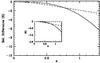Fig. 1 Relative difference between expressions of the luminosity distance. The solid line shows the relative difference between the luminosity distance dL(z) in Eq. (3) and the theoretical luminosity distance in the ΛCDM model in Eq. (6) for ΩM = 0.308 and H0 = 67.8 km s-1 Mpc-1 (Planck Collaboration XIII 2016). The dashed line shows the relative difference between the luminosity distance dL(y), with y ≡ z/ (1 + z), in Cattoën & Visser (2008) and the theoretical luminosity distance in the ΛCDM model. The inset plot shows the corresponding differences in μ, given by Eq. (4), which are indicated by the corresponding line styles.

We now proceed to estimate the parameters { H₀,q₀,j₀ } using the method described in Appendix A of Carvalho & Marques (2016). We assume that at the present epoch c/H₀a₀ ≪ 1, regardless of the value of k, which means that by setting the prior k = 0 and estimating j₀ we are actually estimating j₀ + kc²/ (H₀a₀)² (Neben & Turner 2013). For a model consisting of an incoherent mixture of matter, where each component is described by an equation of state p_i = w_iρ_i, this assumption implies that j₀ ≥ q₀(1 + 2q₀). We also assume that the measurements of the magnitude (and consequently of μ) at different redshifts are independent, which is equivalent to assuming that the parameters’ distribution is Gaussian as a first approximation. We compute the error σ_μdata by assuming uncorrelated errors for the observables and by error propagating according to Eq. (5).

2.1. Global parameter estimation

We first perform a parameter estimation using the complete SN sample, called the global estimation and corresponding to npixel= 1 pixel, from which we estimate the maximum likelihood values for the parameters x_i = { H₀,q₀,j₀ } . (Whenever unspecified, H₀ is measured in units of km s^-1 Mpc^-1.)

For the global estimation, we ran n_j = 10 realizations of Markov chains of length 10⁴. The starting point of each realization is randomly generated. By removing the first 20% of entries in the chains to keep the burnt–in phase only, thinning down the remaining 80% to a half by removing one of each consecutive entry in order to remove correlations within the chain, and finally averaging over the various chains, we obtain the following results: ${\mathit{x}}_{\mathit{i}}^{\mathrm{fid}}\mathrm{=}\mathrm{\left\{}{\mathit{H}}_{\mathrm{0}}^{\mathrm{fid}}\mathit{,}{\mathit{q}}_{\mathrm{0}}^{\mathrm{fid}}\mathit{,}{\mathit{j}}_{\mathrm{0}}^{\mathrm{fid}}\mathrm{\right\}}\mathrm{=}\mathrm{\{}\mathrm{71.06}\mathit{,}\mathrm{-}\mathrm{0.540}\mathit{,}\mathrm{0.533}\mathrm{\}}\mathrm{\pm }\mathrm{\left\{}\mathrm{0.46}\mathit{,}\mathrm{0.094}\mathit{,}\mathrm{0.503}\mathrm{\right\}}$ (see Table 1). We will use these results as the fiducial values in the subsequent calculations. The errors contain the dispersion in each chain and the dispersion among the averages of the different chains added in quadrature.

The measurements of { H₀,q₀,j₀ } are consistent with the measurements of { H₀,q₀ = Ω_M/ 2−Ω_Λ,j₀ = Ω_M + Ω_Λ } obtained in Carvalho & Marques (2016), which we include in Table 1 for convenience. The measurements of { H₀,q₀ } are equally precise, favouring q₀< 0 at over 5σ. The measurement of j₀ is comparatively less precise, as also observed in Neben & Turner (2013) in the context of the kinematic parametrisation, but nonetheless it favours j₀> 0 at 1σ. These results imply that, in the interval z ∈ [0.01,1.30] covered by the SN sample, the cosmic expansion accelerated and that previously it had decelerated, meaning that there was a time when the acceleration changed sign, which supports the evidence found in Riess et al. (2004).

For illustration, in the left panel of Fig. 2 we plot μ_theo computed for the estimated values ${\mathit{x}}_{\mathit{i}}^{\mathrm{fid}}$ as the solid black line. In the right panel we plot the Markov chain of one realization.

We recall that Riess et al. (2004) found q₀ ∈ [−1.3,−0.2] (using the gold sample) which implies j₀ ∈ [−0.3,5.9] , and q₀ ∈ [−1.4,−0.3] (using the combined gold+silver sample) which implies j₀ ∈ [−0.1,6.4] . Moreover, Caldwell & Kamionkowski (2004) found q₀ ∈ [−1.1,−0.2] and j₀ ∈ [−0.5,3.9] . More recent results include Riess et al.’s H₀ = 73.8 ± 2.4 for q₀ = −0.55 and j₀ = 1 using the Hubble Space Telescope set (Riess et al. 2011), and Neben & Turner’s q₀ = −0.64 ± 0.14 and j₀ = 1.4 ± 0.8 using the Constitution set (Neben & Turner 2013). (See Table 1.)

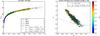Fig. 2 Left panel: distance modulus as a function of redshift. The dots are coloured according to the original SN survey, as described in Betoule et al. (2014), and indicate the distance modulus μdata computed from each SN in the sample. Blue: several low-z. Green: SDSS-II. Yellow: SNLS. Red: HST. The black line indicates the distance modulus computed theoretically for the values { H0,q0,j0 } estimated using the complete sample. The black dashed and black dotted lines indicate the distance modulus for two extreme cases. Right panel: Markov chain of one realization. The dots indicate the entries in the Markov chain. The position in the graph indicates the values of (q0,j0) of each entry according to the axes, whereas the colour indicates the value of H0 as detailed in the side colour bar. The dashed line represents j0 = q0(1 + 2q0), which separates between flat and curved space–time.

2.2. Local parameter estimation

We then divide the SNe over a pixelated map of the sky with pixels of equal surface area according to the HEALPix pixelation (Gorski et al. 2005), and perform a parameter estimation using the SN subsample that falls into each pixel, called the local estimation. The number of pixels that guarantees non–empty SN subsamples in all pixels is npixel= 12 pixels. The number of SNe in each pixel is indicated in Fig. 3 in Carvalho & Marques (2016). Each pixel is assumed to be described by a Friedmann–Lemaître–Roberston–Walker metric so that the full sky is an inhomogeneous ensemble of disjoint, locally homogeneous regions.

For the local estimation, we distinguish two cases as introduced in Carvalho & Marques (2016): the “Cosmic variance” estimation where in each subsample we use the original redshifts and positions, and the “Shuffle SNe” estimation where in each subsample we randomly shuffle the SNe in redshift while keeping the original positions in the sky. The “Shuffle SNe” estimation is hypothesised to be a measure of the noise bias due to the inhomogeneous coverage of the sky by the SN surveys, from which there results inhomogeneity in the SN subsampling. We model this noise bias by the local estimation obtained from randomizing the dependence of redshift with position, while keeping the original SN positions in the sky, and then averaging over the various randomizations.

In each pixel k and for each case of local estimation, we ran n_j = 300 realizations of Markov chains of length 10⁴ and repeated the procedure described above for the global estimation. From the local estimation, there result maps for each estimated parameter x_i with the same pixelation as the SN subsamples, denoted by in the “Cosmic variance” estimation and by $\mathit{x̅}\begin{array}{c}\mathrm{bias}\\ \mathit{ik}\end{array}\mathrm{=}⟨{\mathit{x}}_{\mathit{ijk}}^{\mathrm{bias}}{⟩}_{\mathit{j}}$ in the “Shuffle SNe” estimation, where the brackets denote averaging over the j realizations. Subtracting the noise bias $\mathit{x̅}\begin{array}{c}\mathrm{bias}\\ \mathit{ik}\end{array}$ off we obtain unbiased maps $\mathit{x̅}\begin{array}{c}\mathrm{unbias}\\ \mathit{ik}\end{array}\mathrm{\equiv }\mathit{x̅}{}_{\mathit{ik}}\mathrm{-}\mathit{x̅}\begin{array}{c}\mathrm{bias}\\ \mathit{ik}\end{array}\mathrm{+}{\mathit{x}}_{\mathit{i}}^{\mathrm{fid}}\mathit{.}$ For convenience, we also compare the local estimation with the fiducial values by defining the difference maps $\mathrm{\Delta }\mathit{x̅}{}_{\mathit{ik}}\mathrm{=}\mathit{x̅}{}_{\mathit{ik}}\mathrm{-}{\mathit{x}}_{\mathit{i}}^{\mathrm{fid}}\mathit{,}$ and the unbiased difference maps as $\mathrm{\Delta }\mathit{x̅}\begin{array}{c}\mathrm{unbias}\\ \mathit{ik}\end{array}\mathrm{\equiv }\mathit{x̅}\begin{array}{c}\mathrm{unbias}\\ \mathit{ik}\end{array}\mathrm{-}{\mathit{x}}_{\mathit{i}}^{\mathrm{fid}}\mathrm{=}\mathit{x̅}{}_{\mathit{ik}}\mathrm{-}\mathit{x̅}\begin{array}{c}\mathrm{bias}\\ \mathit{ik}\end{array}\mathit{.}$

The difference maps are shown in Fig. 3 (top panel sets), before (left panel set) and after (right panel set) the noise bias subtraction. Comparing the difference maps with the fiducial values, we measure fluctuations of order 0.1–5% for H₀, 1–187% for q₀ and 1–184% for j₀ before the noise bias subtraction; after the noise bias subtraction, we measure fluctuations of order 0.1–7% for H₀, 1–136% for q₀, and 1–221% for j₀. We recall that Wiegand & Schwarz (2012) found δH₀/H₀^<_~5% using galaxy surveys, which is consistent with our results.

For comparison, in the bottom panels of Fig. 3, we reproduce the difference maps of { H₀,q₀ = Ω_M/ 2−Ω_Λ,j₀ = Ω_M + Ω_Λ } from the { H₀,Ω_M,Ω_Λ } estimation in Carvalho & Marques (2016). We recall that the { H₀,Ω_M,Ω_Λ } estimation yielded fluctuations about the fiducial values of order 0.1–3% for H₀, 0.1–63% for q₀, and 0.001–34% for j₀ before the noise bias subtraction, and fluctuations about the fiducial values of order 0.1–5% for H₀, 0.1–32% for q₀, and 1–27% for j₀ after the noise bias subtraction. This amounts to an increase in the fluctuations by a factor of four and two orders of magnitude respectively before and after the noise bias subtraction, between the { H₀,Ω_M,Ω_Λ } and the { H₀,q₀,j₀ } estimations. The increase in the fluctuations supports the reasoning that accuracy in the estimation of { H₀,q₀ } is compromised by the inclusion of j₀ as an estimated parameter. However, this is also a consequence of using a parametrisation that is independent of the cosmological equation of state, hence of assuming less about the cause of acceleration.

For further comparison, we compute the largest fluctuation in the maps, defined as which yields max( { ΔH₀,Δq₀,Δj₀ } ) = { 5.58,1.27,1.90 } and max( { ΔH₀,Δq₀,Δj₀ } ) = { 6.40,1.31,1.97 } , before and after the noise bias subtraction respectively. We recall that the { H₀,Ω_M,Ω_Λ } estimation yielded max( { ΔH₀,Δq₀,Δj₀ } ) = { 3.84,0.452,0.440 } and max( { ΔH₀,Δq₀,Δj₀ } ) = { 4.40,0.416,0.450 } , before and after the noise bias subtraction respectively. In comparison with the results from other SN studies, namely Kalus et al.’s 2.0 < max(ΔH₀) < 3.4 km s^-1 Mpc^-1 from the Union 2 data for fixed q₀ = −0.601 (Kalus et al. 2013), and Bengaly et al.’s max(ΔH₀) = { 4.6,5.6 } km s^-1 Mpc^-1 and max(Δq₀) = { 2.56,1.62 } respectively from the Union 2.1 data and the JLA data (Bengaly et al. 2015a), we observe that: a) our results for H₀ remain intermediate between the previous results; b) our results for q₀ are intermediate between those of Bengaly et al. (2015a) for the two data sets; and c) our results for j₀ are to the best of our knowledge the first measurements of the kind.

A visual inspection of the pixels through which the Galactic plane crosses does not reveal consistently larger/smaller values of the fluctuations, as also noted in Carvalho & Marques (2016), thus suggesting negligible correlation with the Galactic plane in comparison with the measurement errors (Neben & Turner 2013).

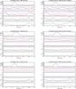Fig. 3 Fluctuations of the estimated parameters as a function of the number of SNe per pixel, before (left panel sets) and after (right panel sets) noise bias removal. Each panel set consists of five panels. At each pixel we plot: a) in the first panel, the number of SNe; b) in the second panel, the value of the parameters { q0,j0 } respectively as the solid red and solid blue lines, with the dashed red and dashed blue lines indicating the corresponding fiducial values; c) in the third panel, the standard deviation { σq0,σj0 } respectively as solid red and solid blue lines; d) in the fourth plot, the value of H0 as the solid black line, with the dashed black line marking the fiducial value; e) in the fifth panel, the standard deviation σH0 as the solid black line. Top panel sets: results from the { H0,q0,j0 } estimation for one pixelation. Centre panel sets: results from the { H0,q0,j0 } estimation for the average over the different pixelations. Bottom panel sets: results from the { H0,ΩM,ΩΛ } estimation for Ωκ = 1−ΩM−ΩΛ.

In order to verify the dependence of the results on the subsampling of the SN surveys per pixel, we perform a test of the effect of rotating the HEALPix pixelation. In particular, starting from the current pixelation and keeping the pixel size constant (i.e. keeping the same number of pixels on the sky), we consider n divisions of each pixel and rotate the pixelation (n_p−1) times in the same direction, the n_pth rotation corresponding to the initial pixelation. At each such rotation by a fraction of 1 /n_p of the pixel, we obtain a different pixelation of the sky and hence a different subsampling of the SN surveys per pixel, totalling n_p different pixelations. We choose n_p = 9 to guarantee a sufficient number of rotations and simultaneously little degeneracy among the rotations.

For each such pixelation p, we perform a local parameter estimation as described above, consisting of a “Cosmic covariance” estimation and a “Shuffle SNe” estimation, and hence obtaining an unbiased parameter estimation in each pixel k,$\mathit{x̅}\begin{array}{c}\mathrm{unbias}\\ \mathit{ikp}\end{array}\mathit{.}$ We then compute the mean unbiased maps averaged over the different pixelations as $\mathit{x̅}\begin{array}{c}\mathrm{unbias}\\ \mathit{ik}\end{array}\mathrm{=}⟨\mathit{x̅}\begin{array}{c}\mathrm{unbias}\\ \mathit{ikp}\end{array}⟩\mathit{,}$ weighted by the inverse of the variance in each pixel, over the different pixelations. From the average over the different pixelations there results a mean pixel derived by averaging the (n−1) rotations of the same pixel in the initial pixelation. For convenience, we define the unbiased difference maps as $\mathrm{\Delta }\mathit{x̅}\begin{array}{c}\mathrm{unbias}\\ \mathit{ik}\end{array}\mathrm{\equiv }\mathit{x̅}\begin{array}{c}\mathrm{unbias}\\ \mathit{ik}\end{array}\mathrm{-}{\mathit{x}}_{\mathit{i}}^{\mathrm{fid}}\mathit{.}$ The resulting difference maps are shown in Fig. 3 centre panel sets, before (left panel set) and after (right panel set) the noise bias subtraction. Comparing the difference maps with the fiducial values, we measure fluctuations of order 0.1–7% for H₀, 0.1–180% for q₀, and 1–116% for j₀ before the noise bias subtraction; after the noise bias subtraction we measure fluctuations of order 0.1–7% for H₀, 0.1–112% for q₀, and 1–135% for j₀. The noise bias removal brings the pixel values closer to the corresponding values estimated from the complete sample, hence decreasing the fluctuations across the sky, albeit increasing slightly the fluctuations in j₀. Simultaneously, it increases the error by up to {10,65,5}% respectively. These results also seem to indicate the validity of $\mathit{x̅}\begin{array}{c}\mathrm{bias}\\ \mathit{ik}\end{array}$ as a measure of the noise bias due to the inhomogeneous SN sampling.

Similarly, the largest fluctuation in the maps yields max({ΔH₀,Δq₀,Δj₀ } ) = {6.01,1.19,1.22} and max({ΔH₀,Δq₀,Δj₀}) = {5.40,1.05,1.27} , before and after the noise bias subtraction.

Hence by averaging over different pixelations of the sample, we obtain a decrease in the fluctuations of the parameters across the sky. However, the mean fluctuations are still larger (by a factor of four and two orders of magnitude respectively before and after the noise bias subtraction) than those obtained in the { H₀,Ω_M,Ω_Λ } estimation. In the subsequent calculations, we will use the parameters’ maps obtained from all n_p pixelations.

3. Power spectra

In order to probe the distribution of the fluctuations by scale, we compute the angular power spectrum of the difference maps normalised to the corresponding fiducial parameter value. The equations below follow closely those in Carvalho & Marques (2016) except for the extra degree of complexity introduced by the different pixelations. In particular, for each parameter x_i and for each realization j of the “Cosmic variance” local estimation, we define the map with value $\mathit{\delta }{\mathit{x}}_{\mathit{ijkp}}\mathrm{\equiv }\mathrm{(}{\mathit{x}}_{\mathit{ijkp}}\mathrm{-}{\mathit{x}}_{\mathit{i}}^{\mathrm{fid}}\mathrm{)}\mathit{/}{\mathit{x}}_{\mathit{i}}^{\mathrm{fid}}$ at each pixel k, for each pixelation p. An estimator of the power spectrum is 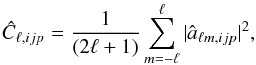$\begin{array}{ccc}\mathit{Ĉ}\mathit{\ell ,ijp}\mathrm{=}\frac{\mathrm{1}}{\mathrm{(}\mathrm{2}\mathit{\ell }\mathrm{+}\mathrm{1}\mathrm{)}}\sum _{\mathit{m}\mathrm{=}\mathrm{-}\mathit{\ell }}^{\mathit{\ell }}\mathrm{|}\mathit{â}\mathit{\ell m,ijp}{\mathrm{|}}^{\mathrm{2}}\mathit{,}& & \end{array}$(7)where the harmonic coefficients â_ℓm,ijp for a pixelated map of N_pix pixels are given by 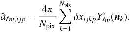$\begin{array}{ccc}\mathit{â}\mathit{\ell m,ijp}\mathrm{=}\frac{\mathrm{4}\mathit{\pi }}{{\mathit{N}}_{\mathrm{pix}}}\sum _{\mathit{k}\mathrm{=}\mathrm{1}}^{{\mathit{N}}_{\mathrm{pix}}}\mathit{\delta }{\mathit{x}}_{\mathit{ijkp}}{\mathit{Y}}_{\mathit{\ell m}}^{\mathrm{\ast }}\mathrm{\left(}{{n}}_{\mathit{k}}\mathrm{\right)}\mathit{.}& & \end{array}$(8)We compute the mean power spectrum Ĉ_ℓ,ip for the parameters { H₀,q₀,j₀ } by averaging the power spectra Ĉ_ℓ,ijp of the maps δx_ijkp = { δH₀,δq₀,δj₀ } _{jkp,cosmic_var} over the j realizations of the “Cosmic variance” local estimation $\begin{array}{ccc}\mathit{Ĉ}\mathit{\ell ,ip}\mathrm{=}⟨\mathit{Ĉ}\mathit{\ell ,ijp}{⟩}_{\mathit{j}}\mathit{,}& & \end{array}$(9)with variance $\begin{array}{ccc}\mathrm{Var}\mathrm{\left[}\mathit{Ĉ}\mathit{\ell ,ip}\mathrm{\right]}\mathrm{=}\mathrm{Var}\mathrm{[}\mathit{Ĉ}\mathit{\ell ,ip}{\mathrm{]}}^{\mathrm{sample}}\mathrm{+}\mathrm{Var}\mathrm{[}\mathit{Ĉ}\mathit{\ell ,ip}{\mathrm{]}}^{\mathrm{estimator}}\mathit{,}& & \end{array}$(10)where $\begin{array}{ccc}\mathrm{Var}\mathrm{[}\mathit{Ĉ}\mathit{\ell ,ip}{\mathrm{]}}^{\mathrm{estimator}}\mathrm{=}\frac{\mathrm{2}}{\mathrm{2}\mathit{\ell }\mathrm{+}\mathrm{1}}\mathit{Ĉ}\begin{array}{c}\mathrm{2}\\ \mathit{\ell ,ip}\end{array}\mathrm{·}& & \end{array}$(11)We then compute the mean power spectrum Ĉ_ℓ,i over the p pixelations $\begin{array}{ccc}\mathit{Ĉ}\mathit{\ell ,i}\mathrm{=}⟨\mathit{Ĉ}\mathit{\ell ,ip}{⟩}_{\mathit{p}}\mathit{,}& & \end{array}$(12)with variance given by $\begin{array}{ccc}\mathrm{Var}\mathrm{\left[}\mathit{Ĉ}\mathit{\ell ,i}\mathrm{\right]}\mathrm{=}{\left[\sum _{\mathit{p}\mathrm{=}\mathrm{1}}^{\mathit{n}}\frac{\mathrm{1}}{\mathrm{Var}\mathrm{\left[}\mathit{Ĉ}\mathit{\ell ,ip}\mathrm{\right]}}\right]}^{-1}\mathrm{·}& & \end{array}$(13)In order to compute the unbiased power spectrum we devise two methods, as detailed below.

3.1. Difference of power spectra

In the first method, we define the unbiased power spectrum as the unbiased mean power spectrum. We compute the unbiased mean power spectrum by computing the power spectrum ${\mathit{C}}_{\mathit{\ell ,ip}}^{\mathrm{bias}}$ of the mean map $\mathit{\delta }\mathit{x̅}\begin{array}{c}\mathrm{bias}\\ \mathit{ikp}\end{array}\mathrm{=}⟨\mathit{\delta }{\mathit{x}}_{\mathit{ijkp}}^{\mathrm{bias}}{⟩}_{\mathit{j}}\mathrm{=}\mathrm{\{}\mathit{\delta }\mathit{H̅}{}_{\mathrm{0}}\mathit{,\delta }\mathit{q̅}{}_{\mathrm{0}}\mathit{,\delta }\mathit{j̅}{}_{\mathrm{0}}\mathrm{\}}_{\mathit{kp,}\mathrm{shuffle\_sn}}$ averaged over the j realizations of the “Shuffle SNe” local estimation and subtracting it from the mean power spectrum Ĉ_ℓ,ip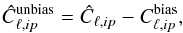$\begin{array}{ccc}\mathit{Ĉ}\begin{array}{c}\mathrm{unbias}\\ \mathit{\ell ,ip}\end{array}\mathrm{=}\mathit{Ĉ}\mathit{\ell ,ip}\mathrm{-}{\mathit{C}}_{\mathit{\ell ,ip}}^{\mathrm{bias}}\mathit{,}& & \end{array}$(14)with total variance $\begin{array}{ccc}\mathrm{Var}\mathrm{\left[}\mathit{Ĉ}\begin{array}{c}\mathrm{unbias}\\ \mathit{\ell ,ip}\end{array}\mathrm{\right]}\mathrm{=}\mathrm{Var}\mathrm{\left[}\mathit{Ĉ}\mathit{\ell ,ip}\mathrm{\right]}\mathrm{+}\mathrm{Var}\mathrm{[}{\mathit{C}}_{\mathit{\ell ,ip}}^{\mathrm{bias}}{\mathrm{]}}^{\mathrm{estimator}}\mathit{.}& & \end{array}$(15)This was the method suggested in Carvalho & Marques (2016). We then compute the mean unbiased power spectrum $\mathit{Ĉ}\begin{array}{c}\mathrm{unbias}\\ \mathit{\ell ,i}\end{array}$ by averaging Ĉ_ℓ,ip over the different p pixelations 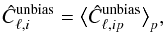$\begin{array}{ccc}\mathit{Ĉ}\begin{array}{c}\mathrm{unbias}\\ \mathit{\ell ,i}\end{array}\mathrm{=}⟨\mathit{Ĉ}\begin{array}{c}\mathrm{unbias}\\ \mathit{\ell ,ip}\end{array}{⟩}_{\mathit{p}}\mathit{,}& & \end{array}$(16)with total variance $\begin{array}{ccc}\mathrm{Var}\mathrm{\left[}\mathit{Ĉ}\begin{array}{c}\mathrm{unbias}\\ \mathit{\ell ,i}\end{array}\mathrm{\right]}\mathrm{=}{\left[\sum _{\mathit{p}\mathrm{=}\mathrm{1}}^{\mathit{n}}\frac{\mathrm{1}}{\mathrm{Var}\mathrm{\left[}\mathit{Ĉ}\begin{array}{c}\mathrm{unbias}\\ \mathit{\ell ,ip}\end{array}\mathrm{\right]}}\right]}^{-1}\mathrm{·}& & \end{array}$(17)In the right panels of Fig. 4, we plot the resulting unbiased power spectra, for the different pixelations and for the average over the p pixelations. The variability in Ĉ_ℓ,ip and ${\mathit{C}}_{\mathit{\ell ,ip}}^{\mathrm{bias}}$ from the different pixelations is indicated as colour-shaded regions bordered by dashed and dotted lines respectively. For all parameters, the power spectrum has a maximum at the quadrupole (ℓ = 2). However, given the size of the error, the results are also compatible with a flat spectrum.

For comparison, in the left panels of Fig. 4, using the same line types, we plot the power spectra for the parameters { H₀,q₀ = Ω_M/ 2−Ω_Λ,j₀ = Ω_M + Ω_Λ } from the { H₀,Ω_M,Ω_Λ } estimation in Carvalho & Marques (2016). In this estimation, the unbiased power spectra also follow the same behaviour as the power spectra before the noise bias removal, with the exception of q₀ whose subtle maximum at ℓ = 2 is erased with the noise bias removal and the power spectrum decreases always with the multipole. Conversely, for H₀ the power spectrum increases always with the multipole, and for j₀ the power spectrum has a maximum at ℓ = 2. Hence, between the { H₀,Ω_M,Ω_Λ } and the { H₀,q₀,j₀ } estimation, we observe the creation of a peak at ℓ = 2 for H₀ and q₀, and the smoothing of the peak for j₀. We also observe that the power spectra in the { H₀,q₀,j₀ } estimation are up to 5 × 10² times the power spectra in the { H₀,Ω_M,Ω_Λ } estimation, hence yielding an increase of the amplitude.

The power spectrum that accounts for the noise bias ${\mathit{C}}_{\mathit{\ell ,i}}^{\mathrm{bias}}$ is up to two orders of magnitude smaller that the mean power spectra Ĉ_ℓ,i, the resulting unbiased mean power spectra $\mathit{Ĉ}\begin{array}{c}\mathrm{unbias}\\ \mathit{\ell ,i}\end{array}$ following the same behaviour as Ĉ_ℓ,i. Since ${\mathit{C}}_{\mathit{\ell ,i}}^{\mathrm{bias}}\mathrm{\ll }\mathit{Ĉ}{}_{\mathit{\ell ,i}}$ for the { H₀,q₀,j₀ } estimation, this method might not remove entirely the noise bias contribution to the power spectrum. For this reason, we conceived another method.

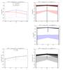Fig. 4 Power spectrum of the parameters estimated from the JLA type Ia SN sample (method A). The dashed lines are the mean power spectra from the “Cosmic variance” estimation, the dotted lines are the power spectra of the average “Shuffle SNe” estimation and the solid lines are the unbiased power spectra defined as the difference between the former two. Left panels: power spectra from the { H0,ΩM,ΩΛ } estimation. Right panels: power spectra from the { H0,q0,j0 } estimation.

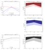Fig. 5 Power spectrum of the parameters estimated from the JLA type Ia SN sample (method B). The dashed lines are the power spectra of the average “Cosmic variance” estimation, the dotted lines are the power spectra of the average “Shuffle SNe” estimation and the solid lines are the unbiased power spectra defined as the power spectra of the average unbiased maps. Left panels: power spectra from the { H0,ΩM,ΩΛ } estimation. Right panels: Power spectra from the { H0,q0,j0 } estimation.

3.2. Power spectrum of unbiased map

In the second method, we define the unbiased power spectrum as the power spectrum of the mean unbiased maps. We compute the unbiased power spectrum by computing the power spectrum ${\mathit{C}}_{\mathit{\ell ,ip}}^{\mathrm{unbias}}$ of the unbiased mean maps $\mathit{\delta }\mathit{x̅}\begin{array}{c}\mathrm{unbias}\\ \mathit{ikp}\end{array}\mathrm{=}\mathrm{(}\mathit{x̅}{}_{\mathit{ikp}}\mathrm{-}\mathit{x̅}\begin{array}{c}\mathrm{bias}\\ \mathit{ikp}\end{array}\mathrm{)}\mathit{/}{\mathit{x}}^{\mathrm{fid}}\mathit{,}$ with total variance $\begin{array}{ccc}\mathrm{Var}\mathrm{\left[}{\mathit{C}}_{\mathit{\ell ,ip}}^{\mathrm{unbias}}\mathrm{\right]}\mathrm{=}\mathrm{Var}\mathrm{[}{\mathit{C}}_{\mathit{\ell ,ip}}^{\mathrm{unbias}}{\mathrm{]}}^{\mathrm{estimator}}\mathit{.}& & \end{array}$(18)We then average over the different p pixelations, defining $\begin{array}{ccc}{\mathit{C}}_{\mathit{\ell ,i}}^{\mathrm{unbias}}\mathrm{=}⟨{\mathit{C}}_{\mathit{\ell ,ip}}^{\mathrm{unbias}}{⟩}_{\mathit{p}}\mathit{,}& & \end{array}$(19)with variance $\begin{array}{ccc}\mathrm{Var}\mathrm{\left[}{\mathit{C}}_{\mathit{\ell ,i}}^{\mathrm{unbias}}\mathrm{\right]}\mathrm{=}{\left[\sum _{\mathit{p}\mathrm{=}\mathrm{1}}^{\mathit{n}}\frac{\mathrm{1}}{\mathrm{Var}\mathrm{\left[}{\mathit{C}}_{\mathit{\ell ,ip}}^{\mathrm{unbias}}\mathrm{\right]}}\right]}^{-1}\mathit{.}& & \end{array}$(20)In the right panels of Fig. 5, we plot the resulting unbiased power spectra, for the different pixelations and the average over the p pixelations. The variability in C_ℓ,ip (the power spectrum of the mean map $\mathit{\delta }\mathit{x̅}{}_{\mathit{ikp}}\mathrm{=}⟨\mathit{\delta }{\mathit{x}}_{\mathit{ijkp}}{⟩}_{\mathit{j}}\mathrm{=}\mathrm{\{}\mathit{\delta }\mathit{H̅}{}_{\mathrm{0}}\mathit{,\delta }\mathit{q̅}{}_{\mathrm{0}}\mathit{,\delta }\mathit{j̅}{}_{\mathrm{0}}\mathrm{\}}_{\mathit{kp,}\mathrm{cosmic\_var}}$ averaged over the j realizations of the “Cosmic variance” local estimation) and ${\mathit{C}}_{\mathit{\ell ,ip}}^{\mathrm{bias}}$ (the power spectrum of the mean map $\mathit{\delta }\mathit{x̅}\begin{array}{c}\mathrm{bias}\\ \mathit{ikp}\end{array}\mathrm{=}⟨\mathit{\delta }{\mathit{x}}_{\mathit{ijkp}}^{\mathrm{bias}}{⟩}_{\mathit{j}}\mathrm{=}\mathrm{\{}\mathit{\delta }\mathit{H̅}{}_{\mathrm{0}}\mathit{,\delta }\mathit{q̅}{}_{\mathrm{0}}\mathit{,\delta }\mathit{j̅}{}_{\mathrm{0}}\mathrm{\}}_{\mathit{kp,}\mathrm{shuffle\_sn}}$ averaged over the j realizations of the “Shuffle SNe” local estimation) from the different pixelations is indicated as colour–shaded regions bordered by dashed and dotted lines respectively and included for reference. For all parameters, the power spectrum has a maximum at ℓ = 2. Although this method has smaller errors than the previous method, the results are still compatible with a flat spectrum.

For comparison, in the left panels of Fig. 5, using the same line types, we plot the power spectra for the parameters { H₀,q₀ = Ω_M/ 2−Ω_Λ,j₀ = Ω_M + Ω_Λ } from the { H₀,Ω_M,Ω_Λ } estimation in Carvalho & Marques (2016). In this estimation, both H₀ and j₀ have a maximum at ℓ = 2, whereas q₀ decreases always with the multipole. Hence, between the { H₀,Ω_M,Ω_Λ } and the { H₀,q₀,j₀ } estimation, we observe the creation of a peak at ℓ = 2 for q₀ and the smoothing of the peak for H₀ and j₀. We also observe that the power spectra in the { H₀,q₀,j₀ } estimation are up to 1 × 10³ times the power spectra in the { H₀,Ω_M,Ω_Λ } estimation, hence yielding an increase of the amplitude.

The two methods return qualitatively equivalent results; quantitatively, however, the second method might be more efficient at removing the noise bias.

4. Average values

In order to compute the average values of the parameters from the corresponding mean maps we average the map of each parameter over the pixel subsamples. When averaging over homogeneous pixels, angular fluctuations in the expansion factor (and consequently in H₀) induce a backreaction term in the average deceleration parameter in the form of an extra positive acceleration (Räsänen 2006). By the same reasoning, angular fluctuations in the expansion factor (and consequently in H₀ and q₀) will also induce a backreaction term in the average jerk parameter. In Carvalho & Marques (2016) we derived the analytical extra positive acceleration for a toy model of an arbitrary number of disjoint, homogeneous regions and computed the overall deceleration parameter assuming a) no backreaction and b) backreaction for the measured angular distribution of H₀. Here, for the same toy model, we derive the corresponding extra terms for the time variation in the acceleration and compute the overall jerk parameter assuming a) no backreaction and b) backreaction for the measured angular distribution of H₀ and q₀.

In the absence of backreaction, the averaging consists in taking the mean weighted by the variance’s inverse of parameter x_i in each pixel k,$\begin{array}{ccc}\mathit{x̅}\mathit{i}\mathrm{=}⟨\mathit{x̅}\mathit{ik}{⟩}_{\mathit{k}}\mathrm{=}\frac{{\sum }_{\mathit{k}}^{{\mathit{N}}_{\mathrm{pixel}}}{\mathit{w}}_{\mathit{k}}\mathit{x̅}\mathit{ik}}{{\sum }_{\mathit{k}}^{{\mathit{N}}_{\mathrm{pixel}}}{\mathit{w}}_{\mathit{k}}}\mathrm{·}& & \end{array}$(21)For the estimated parameters, we find $\mathrm{\left\{}{\overline{\mathit{H}}}_{\mathrm{0}}\mathit{,}{\overline{\mathit{q}}}_{\mathrm{0}}\mathit{,}{\overline{\mathit{j}}}_{\mathrm{0}}\mathrm{\right\}}\mathrm{=}\mathrm{\{}\mathrm{70.99}\mathit{,}\mathrm{-}\mathrm{0.497}\mathit{,}\mathrm{0.538}\mathrm{\}}\mathrm{\pm }\mathrm{\left\{}\mathrm{0.54}\mathit{,}\mathrm{0.126}\mathit{,}\mathrm{0.214}\mathrm{\right\}}\mathit{.}$ After the noise bias removal, we find $\mathrm{\{}{\overline{\mathit{H}}}_{\mathrm{0}}\mathit{,}{\overline{\mathit{q}}}_{\mathrm{0}}\mathit{,}{\overline{\mathit{j}}}_{\mathrm{0}}{\mathrm{\}}}_{\mathrm{unbias}}\mathrm{=}\mathrm{\{}\mathrm{71.32}\mathit{,}\mathrm{-}\mathrm{0.570}\mathit{,}\mathrm{0.540}\mathrm{\}}\mathrm{\pm }\mathrm{\{}\mathrm{0.60}\mathit{,}\mathrm{0.162}\mathit{,}\mathrm{0.333}\mathrm{\}}\mathit{.}$ These values are consistent with the fiducial values. After the noise bias removal, the pixel average values become closer to the corresponding values estimated using the complete sample.

In the presence of backreaction, the averaging consists in taking the mean weighted by the three–volume V_k of each pixel k,$\begin{array}{ccc}\mathit{x̅}\mathit{i}\mathrm{=}⟨\mathit{x̅}\mathit{ik}{⟩}_{{\mathit{V}}_{\mathit{k}}}\mathrm{=}\frac{{\sum }_{\mathit{k}}^{{\mathit{N}}_{\mathrm{pixel}}}{\mathit{V}}_{\mathit{k}}\mathit{x̅}\mathit{ik}}{{\sum }_{\mathit{k}}^{{\mathit{N}}_{\mathrm{pixel}}}{\mathit{V}}_{\mathit{k}}}\mathrm{·}& & \end{array}$(22)Identifying a volume as a pixel and defining v_k = V_k/ ∑ _kV_k, then for N_pixel disjoint regions, the average of the Hubble parameter is given by $\begin{array}{ccc}{⟨{\mathit{H}}_{\mathrm{0}}⟩}_{{\mathit{V}}_{\mathit{k}}}\mathrm{=}\sum _{\mathit{k}}^{{\mathit{N}}_{\mathrm{pixel}}}{\mathit{v}}_{\mathit{k}}{\mathit{H}}_{\mathrm{0}\mathit{,k}}\mathit{.}& & \end{array}$(23)

4.1. Average value of the deceleration parameter

In order to derive the volume average of the acceleration, we take the time derivative of Eq. (23) and find that $\begin{array}{ccc}{⟨\frac{\begin{array}{c}\mathrm{¨}\\ \mathit{a}\end{array}}{\mathit{a}}⟩}_{{\mathit{V}}_{\mathit{k}}}\mathrm{=}\sum _{\mathit{k}}^{{\mathit{N}}_{\mathrm{pixel}}}{\mathit{v}}_{\mathit{k}}\frac{\begin{array}{c}\mathrm{¨}\\ \mathit{a}\end{array}}{\mathit{a}}\mathrm{+}\mathrm{2}\sum _{\mathit{k}}^{{\mathit{N}}_{\mathrm{pixel}}}\sum _{\mathit{l}\mathit{>}\mathit{k}}^{{\mathit{N}}_{\mathrm{pixel}}}{\mathit{v}}_{\mathit{k}}{\mathit{v}}_{\mathit{l}}{\left({\mathit{H}}_{\mathrm{0}\mathit{,k}}\mathrm{-}{\mathit{H}}_{\mathrm{0}\mathit{,l}}\right)}^{\mathrm{2}}\mathit{.}& & \end{array}$(24)Equation (24) decomposes into a linear term in the pixel average of $\mathrm{(}\begin{array}{c}{}_{\mathrm{¨}}\\ \mathit{a}\end{array}\mathit{/}\mathit{a}\mathrm{)}$ and a quadratic term in differences of H₀ between pairs of pixels. The quadratic (backreaction) term generates an acceleration due to the slower regions becoming less represented in the average. In the absence of the quadratic term, the volume average reduces to the pixel average above. Then the volume average of q₀ becomes $\begin{array}{ccc}{⟨{\mathit{q}}_{\mathrm{0}}⟩}_{{\mathit{V}}_{\mathit{k}}}& \mathrm{=}& \sum _{\mathit{k}}^{{\mathit{N}}_{\mathrm{pixel}}}{\mathit{v}}_{\mathit{k}}{\mathit{q}}_{\mathrm{0}\mathit{,k}}\\ & & \end{array}$(25)Using the fluctuations in H₀ (measured in the “Cosmic variance” local estimation) we find and after the noise bias removal we find (see Table 2).

The quadratic term is of order 7 × 10^-4 times the linear term; the corresponding ratio measured in the { H₀,Ω_M,Ω_Λ } estimation was of order 10^-3 (Carvalho & Marques 2016). The difference due to the backreaction is below the standard deviation, hence unobservable. It follows that, for the angular fluctuations in H₀ measured with this SN sample, the contribution of the quadratic term in Eq. (25) is insignificant, which renders the volume averaging equivalent to the pixel averaging. These results confirm that, in the context of this toy model of an inhomogeneous space–time and for a kinetic parametrisation, backreaction is not a viable dynamical mechanism to emulate cosmic acceleration.

4.2. Average value of the jerk parameter

In order to derive the volume average of the time variation in the acceleration, we take the time derivative of Eq. (24) and find that $\begin{array}{ccc}{⟨\frac{\begin{array}{c}\mathrm{...}\\ \mathit{a}\end{array}}{\mathit{a}}⟩}_{{\mathit{V}}_{\mathit{k}}}& \mathrm{=}& \sum _{\mathit{k}}^{{\mathit{N}}_{\mathrm{pixel}}}{\mathit{v}}_{\mathit{k}}\frac{{\begin{array}{c}\mathrm{...}\\ \mathit{a}\end{array}}_{\mathit{k}}}{{\mathit{a}}_{\mathit{k}}}\\ & & \mathrm{+}\mathrm{2}\sum _{\mathit{k}}^{{\mathit{N}}_{\mathrm{pixel}}}\sum _{\mathit{l}\mathit{>}\mathit{k}}^{{\mathit{N}}_{\mathrm{pixel}}}{\mathit{v}}_{\mathit{k}}{\mathit{v}}_{\mathit{l}}{\left({\mathit{H}}_{\mathrm{0}\mathit{,k}}\mathrm{-}{\mathit{H}}_{\mathrm{0}\mathit{,l}}\right)}^{\mathrm{2}}\sum _{\mathit{m}}^{{\mathit{N}}_{\mathrm{pixel}}}{\mathit{v}}_{\mathit{m}}{\mathit{H}}_{\mathrm{0}\mathit{,m}}\\ & & \mathrm{+}\mathrm{2}\sum _{\mathit{k}}^{{\mathit{N}}_{\mathrm{pixel}}}\sum _{\mathit{l}\mathit{>}\mathit{k}}^{{\mathit{N}}_{\mathrm{pixel}}}{\mathit{v}}_{\mathit{k}}{\mathit{v}}_{\mathit{l}}\mathrm{[}\mathrm{(}\mathrm{-}{\mathit{q}}_{\mathrm{0}\mathit{,k}}{{\mathit{H}}_{\mathrm{0}\mathit{,k}}^{\mathrm{2}}}^{\mathrm{)}}\mathrm{-}{\mathrm{(}\mathrm{-}{\mathit{q}}_{\mathrm{0}\mathit{,l}}{{\mathit{H}}_{\mathrm{0}\mathit{,l}}^{\mathrm{2}}}^{\mathrm{)}}}^{\mathrm{]}}\\ & & \end{array}$(26)Equation (26) decomposes into a linear term in the pixel average of $\mathrm{(}\begin{array}{c}\mathrm{...}\\ {}^{\mathit{a}}\end{array}\mathit{/}\mathit{a}\mathrm{)}\mathit{,}$ a quadratic term in differences of H₀ between pairs of pixels and a linear term in differences of $\mathrm{(}\mathrm{-}{\mathit{q}}_{\mathrm{0}}{\mathit{H}}_{\mathrm{0}}^{\mathrm{2}}\mathrm{)}$ between pairs of pixels. The quadratic term in differences of H₀ generates a contribution that is always positive similar to the quadratic term in Eq. (24). Conversely, the linear term in differences of $\mathrm{(}\mathrm{-}{\mathit{q}}_{\mathrm{0}}{\mathit{H}}_{\mathrm{0}}^{\mathrm{2}}\mathrm{)}$ generates a contribution that can have either sign; in particular, it will be positive in the pair of pixels where (− q₀) and H₀ vary in the same direction (i.e. both quantities increase or decrease between pixels) and it will be negative in the pair of pixels where (− q₀) and H₀ vary in opposite directions (i.e. one quantity increases while the other decreases). Since Eq. (26) measures the angular average of the time variation in the acceleration, the difference (backreaction) terms generate an extra jerk that is due to slower regions and/or more slowly varying regions becoming less represented in the average. Similarly to Eq. (24), in the absence of the difference terms, the volume average reduces to the pixel average above. Then the volume average of j₀ becomes 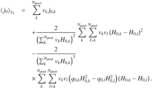$\begin{array}{ccc}{⟨{\mathit{j}}_{\mathrm{0}}⟩}_{{\mathit{V}}_{\mathit{k}}}& \mathrm{=}& \sum _{\mathit{k}}^{{\mathit{N}}_{\mathrm{pixel}}}{\mathit{v}}_{\mathit{k}}{\mathit{j}}_{\mathrm{0}\mathit{,k}}\\ & & \mathrm{+}\frac{\mathrm{2}}{{\left({\sum }_{\mathit{k}}^{{\mathit{N}}_{\mathrm{pixel}}}{\mathit{v}}_{\mathit{k}}{\mathit{H}}_{\mathrm{0}\mathit{,k}}\right)}^{\mathrm{2}}}\sum _{\mathit{k}}^{{\mathit{N}}_{\mathrm{pixel}}}\sum _{\mathit{l}\mathit{>}\mathit{k}}^{{\mathit{N}}_{\mathrm{pixel}}}{\mathit{v}}_{\mathit{k}}{\mathit{v}}_{\mathit{l}}{\left({\mathit{H}}_{\mathrm{0}\mathit{,k}}\mathrm{-}{\mathit{H}}_{\mathrm{0}\mathit{,l}}\right)}^{\mathrm{2}}\\ & & \mathrm{-}\frac{\mathrm{2}}{{\left({\sum }_{\mathit{k}}^{{\mathit{N}}_{\mathrm{pixel}}}{\mathit{v}}_{\mathit{k}}{\mathit{H}}_{\mathrm{0}\mathit{,k}}\right)}^{\mathrm{3}}}\\ & & \end{array}$(27)Using the fluctuations in { H₀,q₀ } (measured in the “Cosmic variance” local parameter estimation), we find and after the noise bias removal, we find (see Table 2).

The quadratic term in differences of H₀ is of order 1 × 10^-3 times the linear term, whereas the linear term in differences of $\mathrm{(}\mathrm{-}{\mathit{q}}_{\mathrm{0}}{\mathit{H}}_{\mathrm{0}}^{\mathrm{2}}\mathrm{)}$ is of order 1 × 10^-2 times the linear term; the corresponding ratios in the { H₀,Ω_M,Ω_Λ } estimation in Carvalho & Marques (2016) were of order 6 × 10^-4 and 2 × 10^-3. Since j₀ is more poorly constrained than q₀ or H₀ in the global estimation, the total difference due to the backreaction is still below the standard deviation, hence unobservable. It follows that, for the angular fluctuations in { H₀,q₀ } measured with this SN sample, the contribution of the backreaction terms in Eq. (27) is insignificant, which renders the pixel averaging equivalent to the pixel averaging. These results imply that an inhomogeneous j₀, such that at different pixels the acceleration changed at different times, cannot be distinguished from a globally homogeneous j₀, such that the acceleration changed everywhere at the same time.

For comparison, we present the pixel average of { q₀ = Ω_M/ 2−Ω_Λ,j₀ = Ω_M + Ω_Λ } from the { H₀,Ω_M,Ω_Λ } estimation in Carvalho & Marques (2016), both in the absence and in the presence of backreaction, which we include in Table 2.

5. Conclusions

In this paper we used SN data to fit a kinematic parametrisation of the luminosity distance expressed in terms of time derivatives of the scale factor. This parametrisation records the cosmic expansion without regard to its cause, thus being independent of the cosmological equation of state and consequently adequate to test interpretations of the cosmic acceleration alternative to the cosmological constant. We followed the parameter estimation, first presented in Carvalho & Marques (2016), to fit the parameters { H₀,q₀,j₀ } by performing both a global and a local parameter estimation. From the global parameter estimation, using the complete SN sample, we obtained the fiducial values adopted in this manuscript. From the local parameter estimation, dividing the SNe into subsamples over a pixelated map, we obtained maps of the estimated parameters with the same pixelation as the SN subsamples. We then proceeded to the analysis of this paper’s results as well as to a comparative analysis with the results from Carvalho & Marques (2016) estimated by fitting { H₀,Ω_M,Ω_Λ } instead.

The measurements of { H₀,q₀,j₀ } are consistent with the measurements of { H₀,q₀ = Ω_M/ 2−Ω_Λ,j₀ = Ω_M + Ω_Λ } obtained in Carvalho & Marques (2016). However, whereas the error of q₀ is of the same order in both parametrisations (about a 5σ measurement), the error of j₀ is significantly larger in the kinematic parametrisation (from a 7σ to a 1σ measurement). This is a consequence of the kinematic parametrisation in part minimising the physical assumptions that enter in the model and in part truncating the Taylor expansion of the luminosity distance.

We measured fluctuations about the average values of order 0.1–5% for H₀, 1–150% for q₀ and 1–124% for j₀. Comparing with the fluctuations measured in Carvalho & Marques (2016), we observe an increase by a factor of two orders of magnitude. We also computed the power spectrum of the corresponding maps of the parameters up to ℓ = 3, as determined by the pixel size, finding that all power spectra have a maximum at ℓ = 2, regardless of the method used to subtract the noise bias. This observation can be partially ascribed to the absence of objects towards the galactic plane.

Finally, for an analytical toy model of an inhomogeneous ensemble of homogenous pixels, we measured the backreaction term in q₀ due to the fluctuations of H₀ to be of order 5 × 10^-4 the corresponding pixel average in the absence of backreaction, hence of smaller order than that measured in Carvalho & Marques (2016). We also derived the backreaction term in j₀ due to the fluctuations of { H₀,q₀ } and measured it to be of order 1 × 10^-2 the corresponding pixel average in the absence of backreaction, hence about 50 times that measured in Carvalho & Marques (2016). However, both backreaction effects are below the corresponding standard deviation and hence rendered unobservable. It follows that backreaction generates insignificant extra acceleration to emulate cosmic acceleration, and insignificant extra jerk to emulate different late–time cosmic histories.

An interesting idea would be to extend this type of analysis to further inhomogeneity studies by combining SN data with other cosmic tracers, such as high–redshift galaxies (Terlevich et al. 2015) and galaxy clusters (Bengaly et al. 2015b; Bolejko et al. 2016).

Acknowledgments

The authors thank A. Afonso and N. Nunes for useful discussions. CSC is funded by Fundação para a Ciência e a Tecnologia (FCT), Grant no. SFRH/BPD/65993/2009.

References

All Tables

All Figures

Fig. 1 Relative difference between expressions of the luminosity distance. The solid line shows the relative difference between the luminosity distance dL(z) in Eq. (3) and the theoretical luminosity distance in the ΛCDM model in Eq. (6) for ΩM = 0.308 and H0 = 67.8 km s-1 Mpc-1 (Planck Collaboration XIII 2016). The dashed line shows the relative difference between the luminosity distance dL(y), with y ≡ z/ (1 + z), in Cattoën & Visser (2008) and the theoretical luminosity distance in the ΛCDM model. The inset plot shows the corresponding differences in μ, given by Eq. (4), which are indicated by the corresponding line styles.

In the text

Fig. 2 Left panel: distance modulus as a function of redshift. The dots are coloured according to the original SN survey, as described in Betoule et al. (2014), and indicate the distance modulus μdata computed from each SN in the sample. Blue: several low-z. Green: SDSS-II. Yellow: SNLS. Red: HST. The black line indicates the distance modulus computed theoretically for the values { H0,q0,j0 } estimated using the complete sample. The black dashed and black dotted lines indicate the distance modulus for two extreme cases. Right panel: Markov chain of one realization. The dots indicate the entries in the Markov chain. The position in the graph indicates the values of (q0,j0) of each entry according to the axes, whereas the colour indicates the value of H0 as detailed in the side colour bar. The dashed line represents j0 = q0(1 + 2q0), which separates between flat and curved space–time.

In the text

Fig. 3 Fluctuations of the estimated parameters as a function of the number of SNe per pixel, before (left panel sets) and after (right panel sets) noise bias removal. Each panel set consists of five panels. At each pixel we plot: a) in the first panel, the number of SNe; b) in the second panel, the value of the parameters { q0,j0 } respectively as the solid red and solid blue lines, with the dashed red and dashed blue lines indicating the corresponding fiducial values; c) in the third panel, the standard deviation { σq0,σj0 } respectively as solid red and solid blue lines; d) in the fourth plot, the value of H0 as the solid black line, with the dashed black line marking the fiducial value; e) in the fifth panel, the standard deviation σH0 as the solid black line. Top panel sets: results from the { H0,q0,j0 } estimation for one pixelation. Centre panel sets: results from the { H0,q0,j0 } estimation for the average over the different pixelations. Bottom panel sets: results from the { H0,ΩM,ΩΛ } estimation for Ωκ = 1−ΩM−ΩΛ.

In the text

Fig. 4 Power spectrum of the parameters estimated from the JLA type Ia SN sample (method A). The dashed lines are the mean power spectra from the “Cosmic variance” estimation, the dotted lines are the power spectra of the average “Shuffle SNe” estimation and the solid lines are the unbiased power spectra defined as the difference between the former two. Left panels: power spectra from the { H0,ΩM,ΩΛ } estimation. Right panels: power spectra from the { H0,q0,j0 } estimation.

In the text

Fig. 5 Power spectrum of the parameters estimated from the JLA type Ia SN sample (method B). The dashed lines are the power spectra of the average “Cosmic variance” estimation, the dotted lines are the power spectra of the average “Shuffle SNe” estimation and the solid lines are the unbiased power spectra defined as the power spectra of the average unbiased maps. Left panels: power spectra from the { H0,ΩM,ΩΛ } estimation. Right panels: Power spectra from the { H0,q0,j0 } estimation.

In the text

References

- Amendola, L., Appleby, S., Bacon, D., et al. 2013, Liv. Rev. Relat., 16, 6 [Google Scholar]
- Aviles, A., Gruber, C., Luongo, O., & Quevedo, H. 2012, Phys. Rev. D, 86, 123516 [NASA ADS] [CrossRef] [Google Scholar]
- Bengaly, C. A. P., Bernui, A., & Alcaniz, J. S. 2015a, ApJ, 808, 39 [NASA ADS] [CrossRef] [Google Scholar]
- Bengaly, C. A. P., Bernui, A., Alcaniz, J. S., & Ferreira, I. S. 2015b, ArXiv eprints [arXiv:1511.09414] [Google Scholar]
- Betoule, M., Kessler, R., Guy, J., et al. 2014, A&A, 568, 22 [Google Scholar]
- Blomqvist, M., Enander, J., & Mortsell, E. 2010, Constraining dark energy fluctuations with supernova correlations, JCAP, 10, 018 [NASA ADS] [CrossRef] [Google Scholar]
- Bolejko, K., Nazer, M. A., & Wiltshire, D. L. 2016, JCAP, 06, 35 [Google Scholar]
- Caldwell, R. R., & Kamionkowski, M. 2004, JCAP, 0409, 009 [NASA ADS] [CrossRef] [Google Scholar]
- Caldwell, R. R., & Stebbins, A. 2008, Phys. Rev. Lett., 100, 191302 [NASA ADS] [CrossRef] [MathSciNet] [PubMed] [Google Scholar]
- Carvalho, C. S., & Marques, K. 2016, A&A, 592, A102 [NASA ADS] [CrossRef] [EDP Sciences] [Google Scholar]
- Cattoën, C., & Visser, M. 2008, Phys. Rev. D, 78, 063501 [NASA ADS] [CrossRef] [Google Scholar]
- Górski, K. M., Hivon, E., Banday, A. J., et al. 2005, ApJ, 622, 759 [NASA ADS] [CrossRef] [Google Scholar]
- Heneka, C., Marra, V., & Amendola, L. 2014, MNRAS, 439, 1855 [NASA ADS] [CrossRef] [Google Scholar]
- Javanmardi, B., Porciani, C., Kroupa, P., & Pflamm-Altenburg, J. 2015, ApJ, 810, 47 [NASA ADS] [CrossRef] [Google Scholar]
- Jiménez, J. B., Salzano, V., & Lazkoz, R. 2015, Phys. Lett. B, 741, 168 [NASA ADS] [CrossRef] [Google Scholar]
- Kalus, B., Schwarz, D. J., Seikel, M., & Wiegand, A. 2013, A&A, 553, A56 [NASA ADS] [CrossRef] [EDP Sciences] [Google Scholar]
- Lan, M. X., Li, M., Li, X. D., & Wang, S. 2010, Phys. Rev. D, 82, 023516 [NASA ADS] [CrossRef] [Google Scholar]
- Liu, S., & Zhang, T. J. 2014, Phys. Lett. B, 733, 69 [NASA ADS] [CrossRef] [Google Scholar]
- Mariano, A., & Perivolaropoulos, L. 2012, Phys. Rev. D, 86, 083517 [NASA ADS] [CrossRef] [Google Scholar]
- Marra, V., & Notari, A. 2011, Class. Quant. Grav., 28, 164004 [NASA ADS] [CrossRef] [Google Scholar]
- Marra, V., & Pääkkönen, M. 2010, JCAP, 1012, 021 [NASA ADS] [CrossRef] [Google Scholar]
- Migkas, K., & Plionis, M. 2016, Rev. Mex. Astron. Astrofis., 52, 133 [Google Scholar]
- Moss, A., Zibin, J. P., & Scott, D. 2011, Phys. Rev. D, 83, 103515 [NASA ADS] [CrossRef] [Google Scholar]
- Neben, A. R., & Turner, M. S. 2013, ApJ, 769, 133 [NASA ADS] [CrossRef] [Google Scholar]
- Planck Collaboration XIII. 2016, A&A, in press, DOI: 10.1051/0004-6361/201525830 [Google Scholar]
- Räsänen, S. 2006, JCAP, 11, 003 [Google Scholar]
- Riess, A. G., Strolger, L. G., Tonry, J., et al. 2004, ApJ, 607, 665 [NASA ADS] [CrossRef] [Google Scholar]
- Riess, A. G., Macri, L., Casterano, S., et al. 2011, ApJ, 730, 119 [NASA ADS] [CrossRef] [Google Scholar]
- Schwarz, D. J., & Weinhorst, B. 2007, A&A, 474, 717 [NASA ADS] [CrossRef] [EDP Sciences] [Google Scholar]
- Terlevich, R., Terlevich, E., Melnick, J., et al. 2015, MNRAS, 451, 3001 [NASA ADS] [CrossRef] [Google Scholar]
- Tomita, K., & Inoue, K. T. 2009, Phys. Rev. D, 79, 103505 [NASA ADS] [CrossRef] [Google Scholar]
- Turner, M. S., & Riess, A. G. 2002, AJ, 569, 18 [NASA ADS] [CrossRef] [Google Scholar]
- Visser, M. 2004, Class. Quant. Grav., 21, 2603 [NASA ADS] [CrossRef] [Google Scholar]
- Wiegand, A., & Schwarz, D. J. 2012, A&A, 538, A147 [NASA ADS] [CrossRef] [EDP Sciences] [Google Scholar]
- Zehavi, I., Riess, A. G., Kirshner, R. P., & Dekel, A. 1998, ApJ, 503, 483 [NASA ADS] [CrossRef] [Google Scholar]
- Zibin, P., Moss, A., & Scott, D. 2008, Phys. Rev. Lett., 101, 251303 [NASA ADS] [CrossRef] [PubMed] [Google Scholar]