| Issue |
A&A
Volume 592, August 2016
|
|
|---|---|---|
| Article Number | A66 | |
| Number of page(s) | 12 | |
| Section | Galactic structure, stellar clusters and populations | |
| DOI | https://doi.org/10.1051/0004-6361/201628502 | |
| Published online | 26 July 2016 | |
Sodium abundances of AGB and RGB stars in Galactic globular clusters
I. Analysis and results of NGC 2808⋆,⋆⋆
1 European Southern Observatory (ESO), Karl-Schwarschild-Str. 2, 85748 Garching b. München, Germany
e-mail: This email address is being protected from spambots. You need JavaScript enabled to view it.
2 Key Laboratory of Optical Astronomy, National Astronomical Observatories, Chinese Academy of Science, 100012 Beijing, PR China
3 School of Astronomy and Space Science, University of Chinese Academy of Sciences, 100049 Beijing, PR China
4 Department of Astronomy, University of Geneva, Chemin des Maillettes 51, 1290 Versoix, Switzerland
5 IRAP, UMR 5277 CNRS and Université de Toulouse, 14 Av. E. Belin, 31400 Toulouse, France
6 Institut d’Astronomie et d’Astrophysique, Université Libre de Bruxelles, CP 226, Boulevard du Triomphe, 1050 Brussels, Belgium
7 Dipartimento di Fisica, Università di Roma Tor Vergata, via della Ricerca Scientifica 1, 00133 Rome, Italy
8 INAF–Osservatorio Astronomico di Roma, via Frascati 33, Monte Porzio Catone, 00133 Rome, Italy
Received: 14 March 2016
Accepted: 22 May 2016
Abstract
Context. Galactic globular clusters (GC) are known to have multiple stellar populations and be characterised by similar chemical features, e.g. O−Na anti-correlation. While second-population stars, identified by their Na overabundance, have been found from the main sequence turn-off up to the tip of the red giant branch (RGB) in various Galactic GCs, asymptotic giant branch (AGB) stars have rarely been targeted. The recent finding that NGC 6752 lacks an Na-rich AGB star has thus triggered new studies on AGB stars in GCs, since this result questions our basic understanding of GC formation and stellar evolution theory.
Aims. We aim to compare the Na abundance distributions of AGB and RGB stars in Galactic GCs and investigate whether the presence of Na-rich stars on the AGB is metallicity-dependent.
Methods. With high-resolution spectra obtained with the multi-object high-resolution spectrograph FLAMES on ESO/VLT, we derived accurate Na abundances for 31 AGB and 40 RGB stars in the Galactic GC NGC 2808.
Results. We find that NGC 2808 has a mean metallicity of −1.11 ± 0.08 dex, in good agreement with earlier analyses. Comparable Na abundance dispersions are derived for our AGB and RGB samples, with the AGB stars being slightly more concentrated than the RGB stars. The ratios of Na-poor first-population to Na-rich second-population stars are 45:55 in the AGB sample and 48:52 in the RGB sample.
Conclusions. NGC 2808 has Na-rich second-population AGB stars, which turn out to be even more numerous − in relative terms − than their Na-poor AGB counterparts and the Na-rich stars on the RGB. Our findings are well reproduced by the fast rotating massive stars scenario and they do not contradict the recent results that there is not an Na-rich AGB star in NGC 6752. NGC 2808 thus joins the larger group of Galactic GCs for which Na-rich second-population stars on the AGB have recently been found.
Key words: stars: abundances / globular clusters: general / globular clusters: individual: NGC 2808
Based on observations made with ESO telescopes at the La Silla Paranal Observatory under programme ID 093.D-0818(A).
Full Tables 2, 4, 6 are only available at the CDS via anonymous ftp to cdsarc.u-strasbg.fr (130.79.128.5) or via http://cdsarc.u-strasbg.fr/viz-bin/qcat?J/A+A/592/A66
© ESO, 2016
1. Introduction
Galactic globular clusters (GC) have been subjected to extensive studies of their chemical characteristics for several decades. In the early 90s, the dedicated Lick-Texas spectroscopic survey of several GCs paved the way and discovered that oxygen and sodium abundances in red giant branch (RGB) stars anti-correlate (e.g. the series by Kraft et al. 1992, 1993, 1995; Sneden et al. 1992, 1994). Later on, the advent of more efficient single/multi-object spectrographs, mounted on 8−10 m class telescopes, allowed for more systematic studies of larger stellar samples down to the turn-off and along the main sequence. Twenty-five years later, the O−Na anti-correlation is recognized as being a chemical feature common to most (if not all, though at different degrees of significance) Galactic GCs (Carretta et al. 2010).
This feature is interpreted as the proof of the existence of (at least) two stellar populations (often referred to as different stellar generations) co-inhabiting the cluster. While first-population (1P) GC stars display Na and O abundances consistent with that of halo field stars of similar metallicity, second-population (2P) stars can be identified by their Na overabundances and O deficiencies that are associated with other chemical peculiarities (e.g. nitrogen and aluminium enrichment, and carbon, lithium, and magnesium deficiency; e.g. Pancino et al. 2010; Villanova & Geisler 2011; Carretta et al. 2014; Carretta 2014; Lapenna et al. 2015). First- and second-population stars are also related to the appearance of multimodal sequences in different regions of GC colour-magnitude diagramme (CMD; e.g. Piotto et al. 2012, 2015; Milone et al. 2015a,b; Nardiello et al. 2015), which can (at least partly) be associated with helium abundance variations in their initial chemical composition (see e.g. Chantereau et al. 2015 and references therein). All these pieces of evidence point to all GCs having suffered from self-enrichment during their early evolution, where 2P stars formed out of the Na-rich, O-poor ashes of hydrogen burning at high temperature ejected by more massive 1P stars and diluted with interstellar gas (e.g. Prantzos & Charbonnel 2006; Prantzos et al. 2007). However, the nature of the polluters remains highly debatable, as well as the mode and timeline of the formation of 2P stars. As of today, none of the proposed models for GC early evolution is able to account for the chemical features that are common to all GCs, nor for the spectrocopic and photometric diversity of these systems (e.g. Bastian et al. 2015; Renzini et al. 2015; Krause et al. 2016). This raises serious challenges related to our understanding of the formation and evolution of massive star clusters and of galaxies in a more general cosmological context.
Therefore, because of the importance of these specific chemical features (like the O−Na anti-correlation), a wealth of observational data has been gathered for a sizable number of Galactic GCs. Cluster stars have been observed and analysed at different evolutionary phases, down to the main sequence, although the majority of the data is from the brighter areas of the CMDs (RGB and HB stars, in particular). Thanks to these analyses, it has been possible to prove the existence of the O−Na anti-correlation at all evolutionary phases in GCs: from the main sequence (MS; e.g. Gratton et al. 2001; Lind et al. 2009; D’Orazi et al. 2010; Monaco et al. 2012; Dobrovolskas et al. 2014) and the subgiant branch (SGB; e.g. Carretta et al. 2005; Lind et al. 2009; Pancino et al. 2011; Monaco et al. 2012) to the red giant branch (RGB; e.g. Yong et al. 2013; Cordero et al. 2014; Carretta et al. 2014, 2015; Gratton et al. 2012a and references therein) and the horizontal branch (HB; e.g. Villanova et al. 2009 and the series by Gratton et al. 2011, 2012b, 2013, 2014, 2015).
However, despite this large number of investigations, asymptotic giant branch (AGB) stars have rarely been targeted systemically because of their paucity in GCs (a result of their short lifetime). Pilachowski et al. (1996) studied a few of them in M 13 (NGC 6205; 112 RGBs, and 18 AGBs) and found them to be rich in sodium ([Na/Fe] > 0.05 dex), similar to the RGB-tip stars (log g< 1) but with a slightly lower overall Na abundance. Johnson & Pilachowski (2012) looked again at the same cluster (M 13) and derived Na and O abundances for 98 RGB and ~15 AGB stars, finding very similar results to Pilachowski et al. (1996), since 66 RGB and twelve AGB stars are in common with the 1996 sample. Since no extreme (very O-poor) AGB star is present in their sample, the authors concluded that only the most Na-rich and O-poor stars may have failed to reach the AGB.
More recently, a spectroscopic study by Campbell et al. (2013) revealed the lack of Na-rich, 2P stars along the early-AGB of NGC 6752. This came as a surprise since, in this GC, as well as all the Milky Way GCs studied so far, 1P and 2P stars have been found at the MS turn-off, on the SGB and on the RGB, and the Na-rich, 2P stars are even twice as numerous as their 1P counterparts (Prantzos & Charbonnel 2006; Carretta et al. 2010). It was therefore concluded by Campbell and collaborators that in NGC 6752 only 1P stars manage to climb the AGB, possibly posing a fundamental problem to stellar evolution theory. This result then triggered a new study of 35 AGB stars in the Galactic GC 47 Tuc (NGC 104, Johnson et al. 2015), which found that, in contrast to NGC 6752, the AGB and RGB populations of 47 Tuc have nearly identical [Na/Fe] dispersions, with only a small fraction (≲ 20%) of Na-rich stars that may fail to ascend the AGB, which is similar to what was observed in M 13. A new study of 6 AGB and 13 RGB stars in M 62 (NGC 6266; Lapenna et al. 2015) find their AGB stars to behave similarly to what was found in NGC 6752, i.e. they are all Na-poor and O-rich (1P) stars. On the other hand, García-Hernández et al. (2015) clearly show that 2P AGB stars exist in metal-poor GCs, with a study of Al and Mg abundances in 44 AGB stars in four metal-poor GCs (M 13, M 5, M 3, and M 2). Therefore, the question of the presence of 2P AGB stars in GCs with various properties (e.g. different ages, metallicities, etc) is far from being settled, although it might bring interesting constraints on the self-enrichment mechanisms (e.g. Charbonnel & Chantereau 2016).
Considering how limited the current sample of GC AGB stars is in terms of Na (and O) abundance determinations, we embarked on a new observational campaign to increase the number of AGB stars for which accurate Na abundances can be derived. We started by observing RGB and AGB stars in NGC 2808, a moderately metal-poor Galactic GC, well known for its multiple stellar populations (e.g. chemically: Carretta et al. 2006; photometrically: Piotto et al. 2007). Thanks to the large number of data available in the literature for NGC 2808, our first goal is to use NGC 2808 as our test-bench cluster, to establish our analysis procedures, before applying the same methodology to a larger number of clusters, spanning a range of metallicities.
The paper is organised as follows: Sects. 2 and 3 describe in detail the observations and the analysis of the data; Sect. 4 presents our derived Na abundance of NGC 2808; the discussion and summary in Sects. 5 and 6 close the paper and suggest future steps; finally, in the Appendix we discuss the influence of different methods to determine the stellar parameters on the derived Na abundances.
2. Observations and data reduction
Our targets were selected from the Johnson-Morgan photometric database that is part of the project described in Stetson (2000, 2005), and cover a magnitude range of about 1.5 mag (V = 15.1−13.5 mag). A total of 53 AGB stars and 47 RGB stars were selected and observed with the high-resolution multi-object spectrograph FLAMES, mounted on ESO/VLT-UT2 (Pasquini et al. 2003). For our programme, we used FLAMES in combined mode, i.e. we observed simultaneously the brightest five objects of our sample with UVES-fibre and the remaining targets with GIRAFFE/Medusa. For UVES-fibre, we chose the Red 580 setting, whereas for GIRAFFE we selected the HR 13, HR 15, and HR 19 set-ups. More details about the observations, which were carried out in service mode, are summarised in Table 1.
Log of the observations for NGC 2808.
Primary data reduction (including the bias correction, wavelength calibration using a Th-Ar lamp, spectrum extraction, and flat fielding) was performed with the ESO GIRAFFE and UVES pipelines, respectively. Sky-subtraction (by averaging seven sky fibres for GIRAFFE sample and one for UVES sample), radial velocity measurement and correction were applied at the end of the reduction procedure. For the GIRAFFE HR 13 and HR 19 spectra, we also performed the telluric correction using the recently released ESO Sky Tool Molecfit (see Smette et al. 2015 and Kausch et al. 2015 for more details). Finally the spectra from the same setup and for the same stars were co-added achieving signal-to-noise ratios (S/N) that range from 100 to 350 for GIRAFFE spectra and 90−180 for UVES spectra, depending on the magnitude of the star.
The barycentric corrections for the radial velocities were derived with the ESO hourly airmass tool1. Figure 1 shows the barycentric radial velocity distribution, as derived for all our observed stars. Although the main peak of the distribution is populated by the majority of our initial sample stars, a long tail towards smaller velocities is also present. We thus only considered as cluster members those stars belonging to the main peak (i.e. all those falling between the two vertical dashed lines in Fig. 1, with barycentric radial velocities of roughly between 85 and 125 km s-1). From this group, we had to further exclude six objects (because of too high metallicity, Fe i and Fe ii abundance mismatches that were incompatible with a reasonable derivation of the reddening, and spectroscopic binary). Our final sample thus consists of 73 stars in total, 33 AGB stars, and 40 RGB stars. Of these, five objects (three AGB and two RGB stars) were observed with UVES−fibre (the UVES sample hereafter) and 68 objects (30 AGB and 38 RGB stars) were observed with FLAMES/GIRAFFE (the GIRAFFE sample hereafter). The mean barycentric radial velocity obtained from all the cluster members is 104.6 km s-1 with a dispersion of σ = 8.0 km s-1, in good agreement with Carretta et al. (2006) (102.4 km s-1 with σ = 9.8 km s-1).
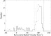 |
Fig. 1 Barycentric radial velocity distribution. The two vertical dashed lines mark the radial velocity range where we select stars as cluster members. |
Table 2 lists the evolutionary phase (AGB/RGB), instrument used for collecting the spectrum (UVES/GIRAFFE), coordinates, photometry, and barycentric radial velocities of our member stars. Their location in the CMD is shown in Fig. 2.
Basic information of our sample stars: evolutionary phase, instrument used for observation, coordinates, photometry, and barycentric radial velocity.
3. Stellar parameters and abundance analysis
3.1. Effective temperature and surface gravity
We used the photometric method to derive the stellar effective temperature (Teff) and surface gravity (log g). Optical B, V, and I magnitudes are available for all our stars. By cross-matching the coordinates of our targets with the 2MASS catalogue (Skrutskie et al. 2006), we have also been able to extract the infrared J, H, and K magnitudes for all except six stars (for which no 2MASS counterpart could be identified).
We adopted the reddening value of E(B−V) = 0.22 mag (Harris 1996, 2010 edition), together with the Cardelli et al. (1989) relations: 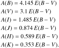 We used the Ramírez & Meléndez (2005) photometric calibrations for giants (which are provided as a function of the colour index and [Fe/H]) and computed five scales of photometric temperatures, using the de-reddened (B−V)0, (V−I)0, (V−J)0, (V−H)0, and (V−K)0 colour indices (see Table 3 for a comparison between the five scales). The mean value of the five temperature scales (Teff,mean) was adopted as our final effective temperature except for the six stars without J, H, and K magnitudes for which we use the mean relation Teff,mean vs. Teff,(V−I), as derived for the rest of the sample.
Mean differences between photometric temperature scales and standard deviations.
To evaluate the error on our final set of effective temperatures, we took into account four main sources of uncertainty: the dispersion σcal of the photometric calibration itself (taken from Ramírez & Meléndez 2005, Table 3; smaller than 40 K for the colours we used); the differential reddening (0.02 mag in E(B−V), Bedin et al. 2000); the uncertainty in the colour index σcolour and on the [Fe/H] ratio. After propagating all errors, we ended up with a typical error on the final Teff of about ± 70 K. The largest contributing source is the differential reddening (~ 55%), followed by the σcal of the calibration itself (~ 33%) and the error on the magnitudes (~ 11%), while the error on the derived metallicity is negligible (about 1%).
The surface gravities log g were derived from effective temperatures and bolometric corrections, assuming that the stars have masses of 0.85 M⊙, as adopted by Carretta et al. (2006). The bolometric corrections of our stars were obtained following the relations by Alonso et al. (1999). We adopted a visual distance modulus of 15.59 mag (Harris 1996, 2010 edition) and the bolometric magnitude of the Sun of Mbol, ⊙ = 4.75. The typical error on log g is about ± 0.05 dex, strongly dominated by the uncertainties in effective temperature (~ 61%) and the differential reddening (~ 39%). The right panel of Fig. 2 shows the final log g−log (Teff) distribution of the member stars.
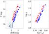 |
Fig. 2 Photometric CMD and log g−log (Teff) distribution. The left panel shows the CMD of the cluster member star sample; and the right panel shows their log g−log (Teff) distribution. The red circles and blue squares represent AGB and RGB stars, respectively, while the GIRAFFE and UVES samples are distinguished by open and filled symbols, respectively. These symbols are used through out this paper. |
3.2. Metallicity and microturbulent velocity
To derive the metallicity [Fe/H] of our stars, we selected unblended Fe i and Fe ii lines from the VALD3 database2 (Piskunov et al. 1995; Kupka et al. 2000; Ryabchikova et al. 2015) where the atomic data was originally taken from Kurucz (2007), Fuhr et al. (1988), O’Brian et al. (1991), Bard et al. (1991), Bard & Kock (1994) for Fe i lines and from Kurucz (2013), and Blackwell et al. (1980), for Fe ii lines, and optimised our selection for GIRAFFE and UVES spectra separately according to their different spectral resolutions and wavelength coverages. The equivalent widths (EWs) of the spectral lines were measured using the automated tool DAOSPEC (Stetson & Pancino 2008), which also outputs the error associated to the derivation of each line equivalent width. To keep the determination of the metallicity as accurate as possible, we excluded very weak (≤ 20 mÅ) and very strong (≥ 120 mÅ) iron lines. We used 1D LTE spherical MARCS model atmospheres (Gustafsson et al. 2008) and the LTE stellar line analysis programme MOOG (Sneden 1973, 2014 release) to derive the metallicity and the microturbulence velocity (ξt), the latter by requiring Fe i abundances to show no trend with the reduced equivalent widths (log (Wλ/λ)) of the lines. An iterative procedure was then followed to consistently derive all stellar parameters (Teff, log g, [Fe/H], and ξt), because of their known interdependences.
We ended up using typically 20−35 Fe i and 4−5 Fe ii lines for the GIRAFFE spectra and 50−65 Fe i and 6−8 Fe ii lines for the UVES spectra. The solar iron abundance of log ϵ(Fe)⊙ = 7.50 from Asplund et al. (2009) is adopted throughout our analysis. Tables 4 and 5 summarise our final stellar parameters and average iron abundances, respectively.
Our derived iron abundances are consistent with those found in the literature (see Table 5). We find a small difference between the [Fe i/H] and [Fe ii/H] ratios, which disappears once we correct the Fe i values for non-LTE corrections (see Sect. 3.4). Therefore, we derive an overall metallicity for NGC 2808 of [Fe /H] =−1.11 dex (rms = 0.09 dex).
Stellar parameters of our sample stars.
Metallicity of NGC 2808 from this work and literature.
Na abundance of our sample stars.
3.3. Sodium abundances
Despite the presence of three different Na i doublets in our spectra (6154−6160 Å in both UVES and GIRAFFE spectra, 8183−8194 Å only in the GIRAFFE spectra, and 5682−5688 Å only in the UVES spectra), we were able to reliably use only the doublet in common to all spectra (i.e. 6154−6160 Å) because the other two show saturation at the metallicity of NGC 2808. This doublet also has a small drawback, namely the 6160 Å line blends with a calcium line, but this can be overcome by analysing the Na doublet via spectrum synthesis.
For this purpose, we used MOOG and our interpolated suite of MARCS model atmospheres, matching our derived stellar parameters. The atomic data of the Na doublet was adopted from the VALD3 database where the data was originally taken from Ralchenko et al. (2010) and Kurucz & Peytremann (1975). Figure 3 shows some examples of observed and synthetic spectra in the Na doublet region for one GIRAFFE AGB star and one UVES RGB star. Considering the overall good agreement between the abundances derived from both lines of the Na doublet, we took the average of the two as our final Na abundance (see Table 6). We note that we have not been able to derive a reliable Na abundance for two out of 33 AGB stars, owing to their lines approaching saturation. By adopting a solar abundance of log ϵ(Na)⊙ = 6.24 (Asplund et al. 2009), we derive a mean cluster Na abundance of [Na/H] =−0.99 dex, with a star-to-star dispersion of rms = 0.19 dex. In more detail, we derive [Na/H] of −1.00 dex (rms = 0.13 dex) and [Na/H] = −0.98 dex (rms = 0.22 dex) for our AGB and RGB samples, respectively.
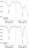 |
Fig. 3 Spectra syntheses of the Na lines region. Top panel: spectra of the GIRAFFE AGB star AGB94048, bottom panel: spectra of the UVES RGB star RGB star RGB112452. The black asterisks represent the observed spectra; the red solid lines are the best-fit synthesised spectra; the blue dash-dotted lines and the green dashed lines are synthesised spectra, but with the best-fit Na abundance changed by plus/minus the error of Na abundance (± 0.07 dex for AGB94048 and ± 0.05 dex for RGB112452; here the error is a combination of random error and fitting error). |
3.4. Non-LTE corrections
Since the line formation of neutral iron is sensitive to departures from local thermodynamic equilibrium (LTE) because of its low fraction in stellar atmospheres, standard LTE analyses of Fe i lines tend to underestimate the true iron abundance, while Fe ii lines are not affected (Lind et al. 2012, and references therein). However, because the iron abundance derived from Fe i lines is statistically more robust owing to the larger number of lines available, we decided to correct our LTE Fe i abundances for the non-LTE (NLTE) effect using the correction grids kindly provided by Lind (priv. comm.), the computation of which is documented in Bergemann et al. (2012) and Lind et al. (2012).
The corrections were calculated for each Fe i line by interpolating the stellar parameters and the EW of the line within the available grids. The top panel of Fig. 4 shows the overall comparison between NLTE and LTE [Fe i/H] and the distribution of the NLTE correction. In Table 7, we list the average LTE and NLTE Fe i abundances, as well as the NLTE corrections, for our AGB and RGB samples respectively. We find that the NLTE correction brings the overall Fe i metallicity of the cluster to [Fe i/H] =−1.11 dex, which is now fully consistent with the value derived from Fe ii lines.
Similar to iron, the lines of neutral sodium also form under non-local thermodynamic equilibrium conditions. For Na, we used the correction grids computed by Lind et al. (2011), which were again applied to each LTE Na line abundance, selecting the exact stellar parameters of the star under investigation. As our final Na abundance per star, we took the average value of the NLTE Na abundances derived from each line of the doublet (see Table 6). The comparison between the NLTE and LTE [Na/H] abundance ratios and the NLTE correction distribution derived for our sample is shown in the bottom panel of Fig. 4. The NLTE correction shifts the Na abundance downwards systematically. The LTE and NLTE [Na/H], together with the NLTE corrections of Na abundance, are also listed in Table 7.
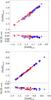 |
Fig. 4 Comparison between NLTE and LTE [Fe i/H] (top panel) and [Na/H] (bottom panel). Each panel is separated into two plots to show a one-to-one comparison (top) and the distribution of the NLTE correction with the LTE abundance (bottom) where the horizontal dashed line marks the mean NLTE correction. Symbols are the same as in Fig. 2. |
LTE and NLTE mean abundances of Fe i and Na of our sample.
3.5. Error analysis
Before discussing our abundance results, we need to estimate the error on the derived abundances. Several sources contribute to the final uncertainty, both of random and systematic nature.
The random measurement uncertainty on the derived abundances can generally be estimated by  , where σ is the line-to-line dispersion and N is the number of lines measured. Here we note that the UVES and GIRAFFE samples have slightly different random uncertainties owing to their different spectral resolutions and λ-coverages. Considering the limited number of Na and Fe ii lines present in our spectra, the application of the above formula is likely less accurate. To compensate for the low number statistics of the Na and Fe ii indicators, we thus applied a correction to the value of according to a t-distribution requiring a 1σ confidence level.
The systematic measurement uncertainty is usually estimated by evaluating the effect on the derived abundances of varying stellar parameters and EWs (or other key parameters of the analysis) by their associated errors, keeping in mind that the stellar parameters are mutually dependent. For this purpose, we selected six representative stars of our samples (GIRAFFE: cool/hot, AGB/RGB, one each; UVES: AGB/RGB, both cool since the UVES sample only has cool stars).
To estimate the systematic influence of the derived stellar parameters, we changed each of the input values (Teff, log g, [M/H], and ξt) in turn, by the amounts corresponding to the uncertainties we derived for each of them (± 70 K, ± 0.05 dex, ± 0.1 dex, and ± 0.1 km s-1 respectively). When changing one parameter, we also iteratively updated all other parameters (see Sect. 3.2). Considering the very similar dependences found for all GIRAFFE and for all UVES stars, Table 8 only gives the “sample”-average values.
For the uncertainty on the individual EW measurements, we adopted the errors estimated by DAOSPEC (edaospec(EW)), which are derived during the least-square fit of a given line. These uncertainties correspond to an average variation of ± 0.04 dex in [Fe i/H] and ± 0.06 dex in [Fe ii/H] for the GIRAFFE sample, and ± 0.02 dex in [Fe i/H] and ± 0.03 dex in [Fe ii/H] for the UVES sample.
For the uncertainties in the Na abundances, which have been determined via spectrum synthesis, we started by shifting the spectra continuum by ± 0.5% and found an average variation of ± 0.06 dex in [Na/H] for the GIRAFFE sample and ± 0.02 dex for the UVES sample. Another possible source of uncertainty is the choice of the atomic physics. Our analysis made use of the atomic parameters of the Na doublet as reported in the VALD3 database, i.e. log (gf) = −1.547 for the Na line at 6154 Å and −1.246 for the one at 6160 Å. No uncertainty is reported for either value, even in the original sources. However, from fitting the solar spectrum with an NLTE model atmosphere, Gehren et al. (2004) derived a slightly different pair of log (gf) values, −1.57 and −1.28 for the 6154 Å and 6160 Å Na lines, respectively. If we now round off this small difference (0.03) to ± 0.05 as our uncertainty on the oscillator strength, we find a ∓ 0.05 dex dependence of the derived [Na/H] ratio for all stars.
Sensitivities of Fe and Na abundances to the variations in stellar parameters.
Table 9 summarises our complete error analysis providing the overall random/systematic/total uncertainties as derived separately for our GIRAFFE and UVES samples by taking the square root of the quadratic sum of the errors associated to all factors, so far discussed. Because the four stellar parameters are mutually dependent, the systematic dependences (and, in turn, the total errors) may be too conservative but they help compensate, at least in part, for those random uncertainties that it is not possible to properly account for. As already mentioned, the difference between the values derived for the two samples (GIRAFFE and UVES) is a consequence of their different spectral resolutions, wavelength coverages, and temperature ranges (e.g. the cool stars observed with UVES only overlap with the coolest stars observed with GIRAFFE).
Uncertainties on the Fe and Na abundances.
In Fig. 3 we show the combined effect of random and fitting errors in the Na abundance (± 0.07 dex for GIRAFFE star and ± 0.05 dex for UVES star) on the synthesised Na line profiles.
3.6. Stars in common with Carretta et al. (2006) work on NGC 2808
By cross-matching target coordinates (within an angular distance of < 0.3′′), we were able to identify 24 RGB stars in common with the sample of Carretta et al. (2006). On average, we find a good agreement on most stellar parameters and abundances. The differences between the two analyses (here, always reported as “this work −Carretta et al. 2006”) are negligible in the stellar parameters, Fe i and Na abundance values3, while for Fe ii amount to + 0.09 ± 0.14 dex. As an example, Fig. 5 shows the comparisons between us and them for both the [Na/H]LTE and [Na/Fe i]LTE ratios.
Applying the sensitivities of Fe and Na abundances to the stellar parameters as reported in Table 8, we can actually account for some of the abundance differences listed above. Small offsets (~+0.05 dex) in Fe ii and Na remain, but they are well within the associated error-bars. We are thus quite confident that our derived abundances are overall in good agreement with those derived by Carretta et al. (2006).
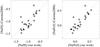 |
Fig. 5 Comparison of [Na/H] and [Na/Fe i] ratio of the common RGB stars between our work and Carretta et al. (2006). Here only LTE abundances are considered. |
The remaining, albeit small, differences could also be due to the different input values and/or methodologies employed by us and by Carretta et al. (2006) (different photometry, Teff-colour calibrations, abundance derivations). Because the final goal of our project is the accurate determination of Na abundances, we think it is important to track these down in more detail. As far as the temperature is concerned, we find a mean ΔTeff = + 44 K because of the different Teff −colour calibrations used, but we note that we are able to reproduce Carretta et al. (2006)Teff and log g values when we adopt their photometry and colour-temperature calibration.
For the Na abundances, the comparison is between spectrum synthesis (ours) and EW-based abundances (Carretta et al. 2006), but it is more cumbersome because we used only the 6154−6160 Å doublet, while Carretta et al. (2006) derived their Na abundances from the EW of different Na doublets, depending on the available spectra. Moreover, the 6160 Å line appears to be severely blended with a neighbouring Ca line on its red wing for several of our RGB stars, making the EW method less reliable. Nonetheless, we find good agreement on the mean values when we derive the Na abundances from the EW of the 6154−6160 Å doublet and with the set of stellar parameters derived according to Carretta et al. (2006) prescriptions (Δ [Na/H] ~ −0.01 ± 0.21 dex, see left panel of Fig. 6), although the amount of scatter persists, mostly as a result of the errors associated with the measurement of the equivalent widths. We also find that, based on our determination of stellar parameters, the spectrum-synthesis-based Na values are, on average, only ~ 0.05 ± 0.07 dex higher than our EW-based values (see. Fig. 6, right panel).
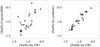 |
Fig. 6 Comparison of [Na/H], as a result of the method test considering the common RGB stars with Carretta et al. (2006). The left panel compares the abundances re-derived by us based on the EWs of the 6154−60 Å doublet and the set of stellar parameters derived according to Carretta et al. (2006) prescriptions with those derived by Carretta et al. (2006). The right panel shows the good agreement between the spectrum-synthesis-based abundances and the (6154−60 Å doublet) EW-based values, based on our own set of stellar parameters. Here only LTE abundances are considered. |
Overall, we can then conclude that the different methods explored so far for the derivation of stellar parameters and/or abundances lead to small systematic differences (within the associated errors in our case), while the errors associated with the EWs/line-fitting measurements are mostly responsible for the dispersions around these values. To complete our diagnostic tests, we have also evaluated the effects of deriving the stellar parameters spectroscopically on our final Na. The results of this test are summarised in the Appendix.
4. Observed Na distribution along the RGB and AGB in NGC 2808
4.1. [Na/H] versus [Na/Fe]
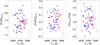 |
Fig. 7 Abundance distributions of our complete (AGB + RGB) sample. Left: [Na/H]NLTE−Teff; middle: [Na/Fe i]NLTE−Teff; right: [NaNLTE/Fe ii]−Teff. Symbols are the same as in Fig. 2. The horizontal dash-dotted lines mark the critical values distinguishing the 1P and 2P stars following Carretta et al. (2009b) criteria (see the text). The typical error bars are shown at the right-bottom corner of each panel (considering the similarity of the errors of the GIRAFFE and UVES samples and the clarity of the figure, we only show the error bars for the GIRAFFE sample which is the largest sample here). |
By comparing the errors in our derived metallicities (σFeI = 0.08 dex) and the star-to-star dispersions (σFeI,obs = 0.09 dex), we find the intrinsic spread in [Fe/H] of NGC 2808 to be within ~ 0.05 dex, when considering only the GIRAFFE sample (representing the large majority of our dataset). The stellar population in NGC 2808 can thus be considered homogeneous in its Fe content within a few hundredths of dex, as also pointed out by Carretta et al. (2006).
Figure 7 shows these effects on the observed abundance patterns, where we present our final Na abundance distributions for AGB and RGB stars in NGC 2808 as [Na/H], [Na/Fe i], and [Na/Fe ii] versus Teff. Overall, the differences among the three panels are minimal. However, because of the extra uncertainties associated with Fe i (due to the NLTE corrections) and Fe ii (due to the paucity of lines), we chose to use the [Na/H] ratio to discuss our derived Na abundance distributions along the RGB and AGB.
4.2. [Na/H] distribution
A quick inspection of Fig. 7 (left panel) shows that the AGB and RGB samples in NGC 2808 have similar Na abundance ranges. A two-sided Kolmogorov-Smirnov (K-S) test confirms this: the K-S statistic D (0.268) and the p-value (0.137) derived for the [Na/H] distribution both indicate that there is only weak evidence to reject the null hypothesis, i.e. the two samples have the same distribution. Examining in more detail the dispersions (σ) and the interquartile range (IQR) values of [Na/H] of the AGB and RGB samples (σAGB = 0.13 and σRGB = 0.21, IQRAGB = 0.16 and IQRRGB = 0.39), we find that the RGB sample is more evenly spread across the entire Na abundance range, while the AGB stars tend to be more concentrated. We also find that the maximum [Na/H] value derived for the AGB sample is 0.21 dex lower than the one derived for the RGB sample. These can be seen in Fig. 8 where we show the histograms and cumulative distributions of [Na/H] for both the AGB and the RGB samples.
The conclusions are relatively similar when we turn to [Na/Fe i] and [Na/Fe ii] (Fig. 7, middle and right). For [Na/Fe i] we obtain (D, p-value) = (0.248, 0.199), σAGB,RGB = (0.16,0.20), IQRAGB,RGB = (0.26,0.39); whereas for [Na/Fe ii] we derive (D, p-value) = (0.224, 0.304), σAGB,RGB = (0.17,0.23) and IQRAGB,RGB = (0.18,0.41).
4.3. Fraction of 1P and 2P stars along the RGB and the AGB
To estimate the relative fraction of 1P vs. 2P stars in our AGB and RGB samples in terms of Na enrichment, we follow Carretta et al. (2009b) who distinguish 1P and 2P stars by identifying those stars that have, respectively, [Na/Fe] below and above [Na/Fe]cri = [Na/Fe]min + 0.3 dex, where [Na/Fe]min is the minimum value of [Na/Fe] derived for the entire sample. We extend this criteria to the absolute abundance and take [Na/H]cri = [Na/H]min + 0.3 dex as the actual reference value to separate 1P and 2P stars. The black dash-dotted lines in Figs. 7 and 8 mark this critical value in each distribution, roughly separating Na-poor 1P from Na-rich 2P stars. It clearly appears that NGC 2808 does host Na-rich 2P AGB stars. When considering the [Na/H] distribution and using the Na cut-off proposed above, the ratio of 1P to 2P stars is 45:55 and 48:52 in the AGB and RGB samples, respectively. As a sanity check, even when [Na/Fe i] or [Na/Fe ii] is considered, one still finds more Na-rich than Na-poor AGB stars, while these two populations are comparable in number along the RGB. Therefore, in our sample, 2P AGB stars are more numerous than 2P RGB stars when compared to their respective 1P counterparts, although they do not reach the same maximum Na abundance as found on the RGB. Furthermore, as far as the RGB stars are concerned, our results agree well with Carretta et al. (2009b) who analysed a much larger RGB star sample (98 stars) and found a 1P:2P stars ratio of 50:50, and even better with Carretta (2015) who reported a similar ratio (1P:2P = 46:54) from the O−Na anti-correlation of 140 RGB stars.
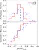 |
Fig. 8 Histograms of [Na/H] (top) and cumulative distribution functions (bottom) of our AGB and RGB sample in NGC 2808. The black vertical dash-dotted line separates 1P and 2P stars using Carretta et al. (2009b) criteria (see text). |
5. Discussion
After the finding by Campbell et al. (2013) that NGC 6752 lacks Na-rich AGB stars, recent studies have revealed a complex chemical picture of AGB stars in Galactic GCs. While another cluster (M 62) was found to be devoid of Na-rich 2P AGB stars, other GCs (NGC 104, M 13, M 5, M 3, and M 2) do have 2P AGB stars (see references in Sect. 1). This work on NGC 2808 adds one more cluster to the latter group. This is particularly interesting, as it provides important constraints on our understanding of the formation and evolution of GCs and of their stellar populations.
It is now largely accepted that GCs suffered from self-enrichment during their early evolution, and that 2P stars formed out of the Na-rich, O-poor ashes of hydrogen burning at high temperature ejected by more massive 1P stars and diluted with interstellar gas (e.g. Prantzos & Charbonnel 2006; Prantzos et al. 2007). Among the most commonly-invoked sources of H-burning ashes, one finds fast-rotating massive stars (FRMS, with initial masses above ~ 25 M⊙; Maeder & Meynet 2006; Prantzos & Charbonnel 2006; Decressin et al. 2007b,a; Krause et al. 2013) and massive AGB stars (with initial masses of ~ 6−11 M⊙; Ventura et al. 2001, 2013; D’Ercole et al. 2010; Ventura & D’Antona 2011). The role of other possible polluters has also been explored: massive stars in close binaries (10−20 M⊙; de Mink et al. 2009; Izzard et al. 2013), FRMS paired with AGB stars (Sills & Glebbeek 2010) or with high-mass interactive binaries (Bastian et al. 2013; Cassisi & Salaris 2014), and supermassive stars (~ 104M⊙; Denissenkov & Hartwick 2014).
The various scenarios for GC self-enrichment differ on many aspects. The most commonly-invoked ones, in particular, make very different predictions for the coupling between Na and He enrichment in the initial composition of 2P stars. In the AGB scenario, on the one hand, all 2P stars spanning a large range in Na are expected to be born with very similar He (maximum ~0.36−0.38 in mass fraction). This is due to the fact that He enrichment in the envelope of the intermediate-mass stellar polluters results from the second dredge-up on the early-AGB before the TP-AGB, where hot bottom-burning might affect the abundances of Na in the polluters yields (e.g. Forestini & Charbonnel 1997; Ventura et al. 2013; Doherty et al. 2014). Therefore within this framework one is expecting to find the same proportion of 1P and 2P stars in the various regions of the GC CMDs, at odds with the observations in NGC 6752.
In the FRMS scenario, on the other hand, the Na and He enrichment of 2P stars at birth are correlated since both chemical elements result from simultaneous H-burning in fast-rotating massive main-sequence stars (Decressin et al. 2007a,b; Chantereau et al. 2015). This has important consequences on the way 1P and 2P stars populate the various sequences of the CMDs. Indeed, owing to the impact of the initial He content of stars on their evolution paths and lifetimes, 2P stars that are born with a chemical composition above an initial He and Na abundances cut-off do not climb the AGB and evolve directly towards the white dwarf stage after central He burning (Chantereau et al. 2015, and in prep.). Therefore, the coupling between He and Na enrichment in the initial composition of 2P stars predicted by the FRMS scenario is expected to lead an evolution of the Na dispersion between the RGB and AGB in individual GCs, in proportions that depend on their age and metallicity (Charbonnel & Chantereau 2016). The corresponding theoretical predictions for an old and relatively metal-poor GC like NGC 6752 ([Fe/H] =−1.54, Campbell et al. 2013; age between ~ 12.5 ± 0.25 Gyr and 13.4 ± 1.1 Gyr according to VandenBerg et al. 2013 and Gratton et al. 2003 respectively) are in good agreement with the lack of Na-rich AGBs in this cluster, although the precise Na-cut-off on the AGB is expected to depend on the assumed RGB mass-loss rate (Charbonnel et al. 2013).
Charbonnel & Chantereau (2016) then showed that within the FRMS scenario the maximum Na content expected for 2P stars on the AGB is a function of both the metallicity and the age of GCs. Namely, at a given [Fe/H], younger clusters are expected to host AGB stars exhibiting a larger Na spread than older clusters; and, at a given age, higher Na dispersion along the AGB is predicted in metal-poor GCs than in the metal-rich ones. NGC 2808 is both younger (11.00 ± 0.38 Gyr by VandenBerg et al. 2013 and 10.9 ± 0.7 Gyr by Massari et al. 2016) and more-metal rich than NGC 6752 and it lies in the domain where RGB and AGB stars are expected to present very similar dispersions, as predicted within the FRMS framework (Charbonnel & Chantereau 2016). Therefore, to first order, the present observations seem to agree well with the theoretically predicted trends.
However, additional parameters may play a role in inducing cluster-to-cluster variations, as already suggested by the spectroscopic and photometric diversity of these complex stellar systems. In particular, mass loss in the earlier phases of stellar evolution (RGB) has been shown to impact the Na cut on the AGB; the higher the mass loss, the stronger the expected differences with age and metallicity between RGB and AGB stars (Charbonnel & Chantereau 2016; see also Cassisi et al. 2014). In addition, the maximum mass of the FRMS polluters might change from cluster to cluster, which should affect their yields and therefore the shape and the extent of the He-Na correlation for 2P stars. It is therefore fundamental to gather additional data in an homegeneous way for GCs spanning a large range in age, metal content, and general properties (mass, compactness, etc) to better constrain the self-enrichment scenarios. Work is in progress in this direction and we will present new Na abundance determinations in three other GCs in the second paper of this series.
6. Summary
The current sample of GC AGB stars available in the literature with accurately derived Na abundances remains rather limited. To increase the number statistics and to further characterise the presence and nature of Na-rich stars on the AGB, we observed and analysed a new sample of 33 AGB and 40 RGB stars in the Galactic GC NGC 2808.
We applied standard analytical methods to derive the stellar parameters and metallicities of the sample. Effective temperatures and stellar gravities were determined photometrically, while the metallicity was derived via equivalent widths of (several) Fe i and (fewer) Fe ii absorption lines. Since the Fe i abundance is affected by the NLTE effect, we applied the NLTE correction, which increased the mean [Fe i/H] by ~ 0.04 dex. Here the [Fe i/H]NLTE and [Fe ii/H] agree well. We thus derived a mean metallicity of NGC 2808 of −1.11 ± 0.08 dex.
We tested the influence on the final Na abundance of adopting photometric vs. spectroscopic methods in the derivation of the stellar parameters. Our test shows that this effect is not significant compared to the various sources of uncertainty, especially when discussing [Na/H] and/or [Na/Fe i] abundance ratios.
Sodium abundances were derived for 31 AGB and 40 RGB stars. From our results, AGB and RGB stars in NGC 2808 have comparable overall Na distributions. By examining the dispersion, the interquartile range and the maximum value of the [Na/H] ratio determined in the AGB and RGB samples, the former appears more concentrated than the latter, in terms of Na abundance ratios.
Following the same criteria as proposed by Carretta et al. (2009b) to separate 1P and 2P GC stars, we derive 1P/2P star ratios of 45:55 (AGB sample) and 48:52 (RGB sample), when the [Na/H] abundance ratio is considered. This result shows that NGC 2808 has an asymptotic giant branch that is populated by relatively larger numbers of Na-rich stars than Na-poor ones, while the two groups are of comparable size on the cluster RGB. This work thus adds another slightly metal-poor GC, NGC 2808, to the group of galactic globular clusters that have Na-rich 2P AGB stars.
When compared to theoretical models, our finding are well accounted for by the FRMS scenario, without being in contradiction with earlier results from, e.g. Campbell et al. (2013). It seems thus important to better quantify the dependences of the Na distributions from cluster metallicity and age. A detailed comparison of Na abundances on the asymptotic giant branch of several GCs and theoretical predictions will be presented in a forthcoming paper (Wang et al., in prep.).
Web interface at http://vald.inasan.ru/~vald3/php/vald.php
ΔTeff = −13 ± 25 K, Δlog g = + 0.02 ± 0.01, Δξt = −0.04 ± 0.18 km s-1, Δ [Fe i/H] LTE = 0.00 ± 0.08 dex, Δ [Na/H] LTE = + 0.04 ± 0.19 dex, and Δ [Na/ Fe i] LTE = + 0.04 ± 0.13 dex.
ξt,spec−ξt,phot = −0.02 ± 0.05 km s-1 and [Fe i/ H] spec− [Fe i/ H] phot = −0.03 ± 0.06 dex. See the text for other parameters and abundances.
Acknowledgments
Y.W. acknowledges the support from the European Southern Observatory, via its ESO Studentship programme. This work was partly funded by the National Natural Science Foundation of China under grants 1233004 and 11390371, as well as the Strategic Priority Research Program The Emergence of Cosmological Structures of the Chinese Academy of Sciences, Grant No. XDB09000000. C.C. and W.C. acknowledge support from the Swiss National Science Foundation (FNS) for the project 200020-159543 Multiple stellar populations in massive star clusters – Formation, evolution, dynamics, impact on galactic evolution. We are indebted to Peter Stetson for kindly providing us with accurate Johnson-Morgan photometry. We thank Karin Lind for useful discussions and for giving us access to her NLTE correction grids. We thank the International Space Science Institute (ISSI, Bern, CH) for welcoming the activities of ISSI Team 271 Massive star clusters across the Hubble Time (2013−2016). This work has made use of the VALD database, operated at Uppsala University, the Institute of Astronomy RAS in Moscow, and the University of Vienna. We thank the anonymous referee for the detailed comments and useful suggestions to improve the paper.
References
- Alonso, A., Arribas, S., & Martínez-Roger, C. 1999, A&AS, 140, 261 [NASA ADS] [CrossRef] [EDP Sciences] [Google Scholar]
- Asplund, M., Grevesse, N., Sauval, A. J., & Scott, P. 2009, ARA&A, 47, 481 [NASA ADS] [CrossRef] [Google Scholar]
- Bard, A., & Kock, M. 1994, A&A, 282, 1014 [NASA ADS] [Google Scholar]
- Bard, A., Kock, A., & Kock, M. 1991, A&A, 248, 315 [NASA ADS] [Google Scholar]
- Bastian, N., Lamers, H. J. G. L. M., de Mink, S. E., et al. 2013, MNRAS, 436, 2398 [NASA ADS] [CrossRef] [MathSciNet] [Google Scholar]
- Bastian, N., Cabrera-Ziri, I., & Salaris, M. 2015, MNRAS, 449, 3333 [NASA ADS] [CrossRef] [Google Scholar]
- Bedin, L. R., Piotto, G., Zoccali, M., et al. 2000, A&A, 363, 159 [NASA ADS] [Google Scholar]
- Bergemann, M., Lind, K., Collet, R., Magic, Z., & Asplund, M. 2012, MNRAS, 427, 27 [NASA ADS] [CrossRef] [Google Scholar]
- Blackwell, D. E., Shallis, M. J., & Simmons, G. J. 1980, A&A, 81, 340 [NASA ADS] [Google Scholar]
- Campbell, S. W., D’Orazi, V., Yong, D., et al. 2013, Nature, 498, 198 [NASA ADS] [CrossRef] [PubMed] [Google Scholar]
- Cardelli, J. A., Clayton, G. C., & Mathis, J. S. 1989, ApJ, 345, 245 [NASA ADS] [CrossRef] [Google Scholar]
- Carretta, E. 2014, ApJ, 795, L28 [NASA ADS] [CrossRef] [Google Scholar]
- Carretta, E. 2015, ApJ, 810, 148 [NASA ADS] [CrossRef] [Google Scholar]
- Carretta, E., Bragaglia, A., & Cacciari, C. 2004, ApJ, 610, L25 [NASA ADS] [CrossRef] [Google Scholar]
- Carretta, E., Gratton, R. G., Lucatello, S., Bragaglia, A., & Bonifacio, P. 2005, A&A, 433, 597 [NASA ADS] [CrossRef] [EDP Sciences] [Google Scholar]
- Carretta, E., Bragaglia, A., Gratton, R. G., et al. 2006, A&A, 450, 523 [NASA ADS] [CrossRef] [EDP Sciences] [Google Scholar]
- Carretta, E., Bragaglia, A., Gratton, R., & Lucatello, S. 2009a, A&A, 505, 139 [NASA ADS] [CrossRef] [EDP Sciences] [Google Scholar]
- Carretta, E., Bragaglia, A., Gratton, R. G., et al. 2009b, A&A, 505, 117 [NASA ADS] [CrossRef] [EDP Sciences] [Google Scholar]
- Carretta, E., Bragaglia, A., Gratton, R. G., et al. 2010, A&A, 516, A55 [NASA ADS] [CrossRef] [EDP Sciences] [Google Scholar]
- Carretta, E., Bragaglia, A., Gratton, R. G., et al. 2014, A&A, 564, A60 [NASA ADS] [CrossRef] [EDP Sciences] [Google Scholar]
- Carretta, E., Bragaglia, A., Gratton, R. G., et al. 2015, A&A, 578, A116 [NASA ADS] [CrossRef] [EDP Sciences] [Google Scholar]
- Cassisi, S., & Salaris, M. 2014, A&A, 563, A10 [NASA ADS] [CrossRef] [EDP Sciences] [Google Scholar]
- Cassisi, S., Salaris, M., Pietrinferni, A., Vink, J. S., & Monelli, M. 2014, A&A, 571, A81 [NASA ADS] [CrossRef] [EDP Sciences] [Google Scholar]
- Chantereau, W., Charbonnel, C., & Decressin, T. 2015, A&A, 578, A117 [NASA ADS] [CrossRef] [EDP Sciences] [Google Scholar]
- Charbonnel, C., & Chantereau, W. 2016, A&A, 586, A21 [NASA ADS] [CrossRef] [EDP Sciences] [Google Scholar]
- Charbonnel, C., Chantereau, W., Decressin, T., Meynet, G., & Schaerer, D. 2013, A&A, 557, L17 [NASA ADS] [CrossRef] [EDP Sciences] [Google Scholar]
- Cordero, M. J., Pilachowski, C. A., Johnson, C. I., et al. 2014, ApJ, 780, 94 [NASA ADS] [CrossRef] [Google Scholar]
- Decressin, T., Charbonnel, C., & Meynet, G. 2007a, A&A, 475, 859 [NASA ADS] [CrossRef] [EDP Sciences] [Google Scholar]
- Decressin, T., Meynet, G., Charbonnel, C., Prantzos, N., & Ekström, S. 2007b, A&A, 464, 1029 [NASA ADS] [CrossRef] [EDP Sciences] [Google Scholar]
- de Mink, S. E., Pols, O. R., Langer, N., & Izzard, R. G. 2009, A&A, 507, L1 [NASA ADS] [CrossRef] [EDP Sciences] [Google Scholar]
- Denissenkov, P. A., & Hartwick, F. D. A. 2014, MNRAS, 437, L21 [NASA ADS] [CrossRef] [Google Scholar]
- D’Ercole, A., D’Antona, F., Ventura, P., Vesperini, E., & McMillan, S. L. W. 2010, MNRAS, 407, 854 [NASA ADS] [CrossRef] [MathSciNet] [Google Scholar]
- Dobrovolskas, V., Kučinskas, A., Bonifacio, P., et al. 2014, A&A, 565, A121 [NASA ADS] [CrossRef] [EDP Sciences] [Google Scholar]
- Doherty, C. L., Gil-Pons, P., Lau, H. H. B., Lattanzio, J. C., & Siess, L. 2014, MNRAS, 437, 195 [NASA ADS] [CrossRef] [Google Scholar]
- D’Orazi, V., Lucatello, S., Gratton, R., et al. 2010, ApJ, 713, L1 [NASA ADS] [CrossRef] [Google Scholar]
- Forestini, M., & Charbonnel, C. 1997, A&AS, 123 [Google Scholar]
- Fuhr, J. R., Martin, G. A., & Wiese, W. L. 1988, J. Phys. Chem. Ref. Data (New York: AIP and American Chemical Society), Vol. 17 [Google Scholar]
- García-Hernández, D. A., Mészáros, S., Monelli, M., et al. 2015, ApJ, 815, L4 [NASA ADS] [CrossRef] [Google Scholar]
- Gehren, T., Liang, Y. C., Shi, J. R., Zhang, H. W., & Zhao, G. 2004, A&A, 413, 1045 [NASA ADS] [CrossRef] [EDP Sciences] [Google Scholar]
- Gratton, R. G., Bonifacio, P., Bragaglia, A., et al. 2001, A&A, 369, 87 [NASA ADS] [CrossRef] [EDP Sciences] [Google Scholar]
- Gratton, R. G., Bragaglia, A., Carretta, E., et al. 2003, A&A, 408, 529 [NASA ADS] [CrossRef] [EDP Sciences] [Google Scholar]
- Gratton, R. G., Lucatello, S., Carretta, E., et al. 2011, A&A, 534, A123 [NASA ADS] [CrossRef] [EDP Sciences] [Google Scholar]
- Gratton, R. G., Carretta, E., & Bragaglia, A. 2012a, A&ARv, 20, 50 [CrossRef] [Google Scholar]
- Gratton, R. G., Lucatello, S., Carretta, E., et al. 2012b, A&A, 539, A19 [NASA ADS] [CrossRef] [EDP Sciences] [Google Scholar]
- Gratton, R. G., Lucatello, S., Sollima, A., et al. 2013, A&A, 549, A41 [NASA ADS] [CrossRef] [EDP Sciences] [Google Scholar]
- Gratton, R. G., Lucatello, S., Sollima, A., et al. 2014, A&A, 563, A13 [NASA ADS] [CrossRef] [EDP Sciences] [Google Scholar]
- Gratton, R. G., Lucatello, S., Sollima, A., et al. 2015, A&A, 573, A92 [NASA ADS] [CrossRef] [EDP Sciences] [Google Scholar]
- Gustafsson, B., Edvardsson, B., Eriksson, K., et al. 2008, A&A, 486, 951 [NASA ADS] [CrossRef] [EDP Sciences] [Google Scholar]
- Harris, W. E. 1996, AJ, 112, 1487 [NASA ADS] [CrossRef] [Google Scholar]
- Izzard, R. G., de Mink, S. E., Pols, O. R., et al. 2013, Mem. Soc. Astron. It., 84, 171 [NASA ADS] [Google Scholar]
- Johnson, C. I., & Pilachowski, C. A. 2012, ApJ, 754, L38 [NASA ADS] [CrossRef] [Google Scholar]
- Johnson, C. I., McDonald, I., Pilachowski, C. A., et al. 2015, AJ, 149, 71 [NASA ADS] [CrossRef] [Google Scholar]
- Kausch, W., Noll, S., Smette, A., et al. 2015, A&A, 576, A78 [NASA ADS] [CrossRef] [EDP Sciences] [Google Scholar]
- Kraft, R. P., Sneden, C., Langer, G. E., & Prosser, C. F. 1992, AJ, 104, 645 [NASA ADS] [CrossRef] [Google Scholar]
- Kraft, R. P., Sneden, C., Langer, G. E., & Shetrone, M. D. 1993, AJ, 106, 1490 [NASA ADS] [CrossRef] [Google Scholar]
- Kraft, R. P., Sneden, C., Langer, G. E., Shetrone, M. D., & Bolte, M. 1995, AJ, 109, 2586 [NASA ADS] [CrossRef] [Google Scholar]
- Krause, M., Charbonnel, C., Decressin, T., Meynet, G., & Prantzos, N. 2013, A&A, 552, A121 [NASA ADS] [CrossRef] [EDP Sciences] [Google Scholar]
- Krause, M. G. H., Charbonnel, C., Bastian, N., & Diehl, R. 2016, A&A, 587, A53 [NASA ADS] [CrossRef] [EDP Sciences] [Google Scholar]
- Kupka, F. G., Ryabchikova, T. A., Piskunov, N. E., Stempels, H. C., & Weiss, W. W. 2000, Balt. Astron., 9, 590 [NASA ADS] [Google Scholar]
- Kurucz, R. L. 2007, Robert L. Kurucz on-line database of observed and predicted atomic transitions [Google Scholar]
- Kurucz, R. L. 2013, Robert L. Kurucz on-line database of observed and predicted atomic transitions [Google Scholar]
- Kurucz, R. L., & Peytremann, E. 1975, SAO Special Report, 362, 1 [Google Scholar]
- Lind, K., Primas, F., Charbonnel, C., Grundahl, F., & Asplund, M. 2009, A&A, 503, 545 [NASA ADS] [CrossRef] [EDP Sciences] [MathSciNet] [Google Scholar]
- Lind, K., Asplund, M., Barklem, P. S., & Belyaev, A. K. 2011, A&A, 528, A103 [Google Scholar]
- Lind, K., Bergemann, M., & Asplund, M. 2012, MNRAS, 427, 50 [NASA ADS] [CrossRef] [Google Scholar]
- Lapenna, E., Mucciarelli, A., Ferraro, F. R., et al. 2015, ApJ, 813, 97 [CrossRef] [Google Scholar]
- Maeder, A., & Meynet, G. 2006, A&A, 448, L37 [NASA ADS] [CrossRef] [EDP Sciences] [Google Scholar]
- Massari, D., Fiorentino, G., McConnachie, A., et al. 2016, A&A, 586, A51 [NASA ADS] [CrossRef] [EDP Sciences] [Google Scholar]
- Milone, A. P., Marino, A. F., Piotto, G., et al. 2015a, MNRAS, 447, 927 [NASA ADS] [CrossRef] [Google Scholar]
- Milone, A. P., Marino, A. F., Piotto, G., et al. 2015b, ApJ, 808, 51 [NASA ADS] [CrossRef] [Google Scholar]
- Monaco, L., Villanova, S., Bonifacio, P., et al. 2012, A&A, 539, A157 [NASA ADS] [CrossRef] [EDP Sciences] [Google Scholar]
- Nardiello, D., Piotto, G., Milone, A. P., et al. 2015, MNRAS, 451, 312 [NASA ADS] [CrossRef] [Google Scholar]
- O’Brian, T. R., Wickliffe, M. E., Lawler, J. E., Whaling, W., & Brault, J. W. 1991, J. Opt. Soc. Am. B Opt. Phys., 8, 1185 [NASA ADS] [CrossRef] [Google Scholar]
- Pancino, E., Rejkuba, M., Zoccali, M., & Carrera, R. 2010, A&A, 524, A44 [NASA ADS] [CrossRef] [EDP Sciences] [Google Scholar]
- Pancino, E., Mucciarelli, A., Sbordone, L., et al. 2011, A&A, 527, A18 [NASA ADS] [CrossRef] [EDP Sciences] [Google Scholar]
- Pasquini, L., Alonso, J., Avila, G., et al. 2003, in Instrument Design and Performance for Optical/Infrared Ground-based Telescopes, eds. M. Iye, & A. F. M. Moorwood, SPIE Conf. Ser., 4841, 1682 [Google Scholar]
- Pilachowski, C. A., Sneden, C., Kraft, R. P., & Langer, G. E. 1996, AJ, 112, 545 [NASA ADS] [CrossRef] [Google Scholar]
- Piotto, G., Bedin, L. R., Anderson, J., et al. 2007, ApJ, 661, L53 [NASA ADS] [CrossRef] [Google Scholar]
- Piotto, G., Milone, A. P., Anderson, J., et al. 2012, ApJ, 760, 39 [NASA ADS] [CrossRef] [Google Scholar]
- Piotto, G., Milone, A. P., Bedin, L. R., et al. 2015, AJ, 149, 91 [NASA ADS] [CrossRef] [Google Scholar]
- Piskunov, N. E., Kupka, F., Ryabchikova, T. A., Weiss, W. W., & Jeffery, C. S. 1995, A&AS, 112, 525 [NASA ADS] [Google Scholar]
- Prantzos, N., & Charbonnel, C. 2006, A&A, 458, 135 [NASA ADS] [CrossRef] [EDP Sciences] [Google Scholar]
- Prantzos, N., Charbonnel, C., & Iliadis, C. 2007, A&A, 470, 179 [NASA ADS] [CrossRef] [EDP Sciences] [Google Scholar]
- Ralchenko, Y., Kramida, A., Reader, J., & NIST ASD Team 2010, NIST Atomic Spectra Database (ver. 4.0.0) [Google Scholar]
- Ramírez, I., & Meléndez, J. 2005, ApJ, 626, 465 [NASA ADS] [CrossRef] [Google Scholar]
- Renzini, A., D’Antona, F., Cassisi, S., et al. 2015, MNRAS, 454, 4197 [NASA ADS] [CrossRef] [Google Scholar]
- Ryabchikova, T., Piskunov, N., Kurucz, R. L., et al. 2015, Phys. Scr., 90, 054005 [NASA ADS] [CrossRef] [Google Scholar]
- Sills, A., & Glebbeek, E. 2010, MNRAS, 407, 277 [NASA ADS] [CrossRef] [Google Scholar]
- Skrutskie, M. F., Cutri, R. M., Stiening, R., et al. 2006, AJ, 131, 1163 [NASA ADS] [CrossRef] [Google Scholar]
- Smette, A., Sana, H., Noll, S., et al. 2015, A&A, 576, A77 [NASA ADS] [CrossRef] [EDP Sciences] [Google Scholar]
- Sneden, C. A. 1973, Ph.D. Thesis, the University of Texas at Austin [Google Scholar]
- Sneden, C., Kraft, R. P., Prosser, C. F., & Langer, G. E. 1992, AJ, 104, 2121 [NASA ADS] [CrossRef] [Google Scholar]
- Sneden, C., Kraft, R. P., Langer, G. E., Prosser, C. F., & Shetrone, M. D. 1994, AJ, 107, 1773 [NASA ADS] [CrossRef] [Google Scholar]
- Stetson, P. B. 2000, PASP, 112, 925 [NASA ADS] [CrossRef] [Google Scholar]
- Stetson, P. B. 2005, PASP, 117, 563 [CrossRef] [Google Scholar]
- Stetson, P. B., & Pancino, E. 2008, PASP, 120, 1332 [Google Scholar]
- VandenBerg, D. A., Brogaard, K., Leaman, R., & Casagrande, L. 2013, ApJ, 775, 134 [NASA ADS] [CrossRef] [Google Scholar]
- Ventura, P., & D’Antona, F. 2011, MNRAS, 410, 2760 [NASA ADS] [CrossRef] [Google Scholar]
- Ventura, P., D’Antona, F., Mazzitelli, I., & Gratton, R. 2001, ApJ, 550, L65 [NASA ADS] [CrossRef] [Google Scholar]
- Ventura, P., Di Criscienzo, M., Carini, R., & D’Antona, F. 2013, MNRAS, 431, 3642 [NASA ADS] [CrossRef] [Google Scholar]
- Villanova, S., & Geisler, D. 2011, A&A, 535, A31 [NASA ADS] [CrossRef] [EDP Sciences] [Google Scholar]
- Villanova, S., Piotto, G., & Gratton, R. G. 2009, A&A, 499, 755 [NASA ADS] [CrossRef] [EDP Sciences] [Google Scholar]
- Yong, D., Meléndez, J., Grundahl, F., et al. 2013, MNRAS, 434, 3542 [NASA ADS] [CrossRef] [Google Scholar]
Appendix A: Spectroscopic stellar parameters
We selected ten stars (4 AGB and 6 RGB) representative of our GIRAFFE sample (i.e. covering their entire temperature ranges). We then derived the (excitation) temperature, by requiring a null slope between the Fe i abundances and the excitation potential of the individual Fe i lines (the so-called excitation equilibrium) and the surface gravity, by requiring Fe i and Fe ii lines to give the same abundance (the so-called ionization equilibrium). Stellar metallicity and microturbulent velocities were determined, as described in Sect. 3.2. We note that by imposing the ionisation balance between Fe iNLTE and Fe ii (i.e. taking somehow into account a mean NLTE correction to Fe i of ≃0.04 dex) only the gravity and the Fe ii abundance are slightly affected (log g by + 0.08 dex − from LTE to NLTE − and Fe ii by + 0.05 dex).
As far as the temperature is concerned, we find a mean difference that is smaller than our estimated error on this parameter (Tspec−Tphot = −26 ± 56 K). The standard deviation around the mean value, however, hints to possibly important dependencies on the type of star: the temperature difference is slightly larger in the AGB stars (−34 K) than in the RGB ones (−26 K); cool stars (AGB and RGB) show positive differences, while the hotter ones tend to be negative. This is observed also for all the
other parameters (surface gravity and microturbulent velocity) and abundances (Fe i, Fe ii, Na i)4, with the surface gravity being the most affected quantity.
On average, the ionisation equilibrium requirement (omitting the NLTE effect on Fe i) decreases log g by −0.14 ± 0.24 dex and the Fe ii abundance by −0.05 ± 0.09 dex with respect to the photometry-based result. The differences on log g and Fe ii decrease to −0.06 ± 0.2 dex and −0.01 ± 0.09 dex respectively, when we apply NLTE corrections to the Fe i values before seeking for the ionisation balance. The Fe i abundances differ by −0.03 ± 0.6 dex between the spectroscopic (lower) and photometric results, independently of the NLTE correction.
When deriving the Na abundances (we used the EWs of the 6154−6160 Å Na doublet for the purpose of this test) with the spectroscopic set of stellar parameters, we find a negligible difference on the derived [Na/H] ratios (Δ = −0.02, rms = 0.04 dex, with the spectroscopic one being lower). This is much smaller than their associated errors and the difference between AGB and RGB samples is negligible.
In summary, the effect of applying a photometric or spectroscopic method to derive stellar parameters and abundances is not significant and the resulting sets of abundances agree well within the associated errors.
All Tables
Basic information of our sample stars: evolutionary phase, instrument used for observation, coordinates, photometry, and barycentric radial velocity.
All Figures
|
Fig. 1 Barycentric radial velocity distribution. The two vertical dashed lines mark the radial velocity range where we select stars as cluster members. |
| In the text | |
|
Fig. 2 Photometric CMD and log g−log (Teff) distribution. The left panel shows the CMD of the cluster member star sample; and the right panel shows their log g−log (Teff) distribution. The red circles and blue squares represent AGB and RGB stars, respectively, while the GIRAFFE and UVES samples are distinguished by open and filled symbols, respectively. These symbols are used through out this paper. |
| In the text | |
|
Fig. 3 Spectra syntheses of the Na lines region. Top panel: spectra of the GIRAFFE AGB star AGB94048, bottom panel: spectra of the UVES RGB star RGB star RGB112452. The black asterisks represent the observed spectra; the red solid lines are the best-fit synthesised spectra; the blue dash-dotted lines and the green dashed lines are synthesised spectra, but with the best-fit Na abundance changed by plus/minus the error of Na abundance (± 0.07 dex for AGB94048 and ± 0.05 dex for RGB112452; here the error is a combination of random error and fitting error). |
| In the text | |
|
Fig. 4 Comparison between NLTE and LTE [Fe i/H] (top panel) and [Na/H] (bottom panel). Each panel is separated into two plots to show a one-to-one comparison (top) and the distribution of the NLTE correction with the LTE abundance (bottom) where the horizontal dashed line marks the mean NLTE correction. Symbols are the same as in Fig. 2. |
| In the text | |
|
Fig. 5 Comparison of [Na/H] and [Na/Fe i] ratio of the common RGB stars between our work and Carretta et al. (2006). Here only LTE abundances are considered. |
| In the text | |
|
Fig. 6 Comparison of [Na/H], as a result of the method test considering the common RGB stars with Carretta et al. (2006). The left panel compares the abundances re-derived by us based on the EWs of the 6154−60 Å doublet and the set of stellar parameters derived according to Carretta et al. (2006) prescriptions with those derived by Carretta et al. (2006). The right panel shows the good agreement between the spectrum-synthesis-based abundances and the (6154−60 Å doublet) EW-based values, based on our own set of stellar parameters. Here only LTE abundances are considered. |
| In the text | |
|
Fig. 7 Abundance distributions of our complete (AGB + RGB) sample. Left: [Na/H]NLTE−Teff; middle: [Na/Fe i]NLTE−Teff; right: [NaNLTE/Fe ii]−Teff. Symbols are the same as in Fig. 2. The horizontal dash-dotted lines mark the critical values distinguishing the 1P and 2P stars following Carretta et al. (2009b) criteria (see the text). The typical error bars are shown at the right-bottom corner of each panel (considering the similarity of the errors of the GIRAFFE and UVES samples and the clarity of the figure, we only show the error bars for the GIRAFFE sample which is the largest sample here). |
| In the text | |
|
Fig. 8 Histograms of [Na/H] (top) and cumulative distribution functions (bottom) of our AGB and RGB sample in NGC 2808. The black vertical dash-dotted line separates 1P and 2P stars using Carretta et al. (2009b) criteria (see text). |
| In the text | |
Current usage metrics show cumulative count of Article Views (full-text article views including HTML views, PDF and ePub downloads, according to the available data) and Abstracts Views on Vision4Press platform.
Data correspond to usage on the plateform after 2015. The current usage metrics is available 48-96 hours after online publication and is updated daily on week days.
Initial download of the metrics may take a while.