| Issue |
A&A
Volume 592, August 2016
|
|
|---|---|---|
| Article Number | A40 | |
| Number of page(s) | 16 | |
| Section | Astrophysical processes | |
| DOI | https://doi.org/10.1051/0004-6361/201628351 | |
| Published online | 18 July 2016 | |
Time-varying sodium absorption in the Type Ia supernova 2013gh⋆
1 Department of Physics, The Oskar Klein Centre, Stockholm University, Albanova, 106 92 Stockholm, Sweden
e-mail: raphael.ferretti@fysik.su.se
2 Department of Particle Physics and Astrophysics, Weizmann Institute of Science, 7610001 Rehovot, Israel
3 Department of Terrestrial Magnetism, Carnegie Institute of Washington, Washington, DC 20015, USA
4 Cahill Center for Astrophysics, California Institute of Technology, Pasadena, CA 91125, USA
5 Astrophysics Science Division, NASA Goddard Space Flight Center, Mail Code 661, Greenbelt, MD 20771, USA
6 Joint Space-Science Institute, University of Maryland, College Park, MD 20742, USA
7 Jet Propulsion Laboratory, California Institute of Technology, Pasadena, CA 91109, USA
8 Department of Astronomy, University of California, Berkeley, CA 94720-3411, USA
9 Department of Astronomy, The Oskar Klein Center, Stockholm University, Albanova, 10691 Stockholm, Sweden
10 Department of Physics, University of California, Santa Barbara, CA 93106-9530, USA
11 Las Cumbres Observatory Global Telescope Network, 6740 Cortona Dr., Suite 102, Goleta, CA 93117, USA
12 Tuorla Observatory, Department of Physics and Astronomy, University of Turku, Väisäläntie 20, 21500 Piikkiö, Finland
13 Finnish Centre for Astronomy with ESO (FINCA), University of Turku, Väisäläntie 20, 21500 Piikkiö, Finland
14 Institute of Astronomy, University of Cambridge, Madingley Road, Cambridge, CB3 0HA, UK
15 Humboldt-Universität zu Berlin, Institut für Physik, Newtonstrasse 15, 12589 Berlin, Germany
16 Lawrence Berkeley National Laboratory, 1 Cyclotron Road, MS 50B-4206, Berkeley, CA 94720, USA
17 Department of Physics, University of California, One Shields Avenue, Davis, CA 95616, USA
18 UCO/Lick Observatory, Department of Astronomy and Astrophysics, University of California, Santa Cruz, CA 95064, USA
19 Los Alamos National Laboratory, MS D436, Los Alamos, NM 87545, USA
Received: 19 February 2016
Accepted: 2 May 2016
Context. Temporal variability of narrow absorption lines in high-resolution spectra of Type Ia supernovae (SNe Ia) is studied to search for circumstellar matter. Time series which resolve the profiles of absorption lines such as Na I D or Ca II H&K are expected to reveal variations due to photoionisation and subsequent recombination of the gases. The presence, composition, and geometry of circumstellar matter may hint at the elusive progenitor system of SNe Ia and could also affect the observed reddening law.
Aims. To date, there are few known cases of time-varying Na I D absorption in SNe Ia, all of which occurred during relatively late phases of the supernova (SN) evolution. Photoionisation, however, is predicted to occur during the early phases of SNe Ia, when the supernovae peak in the ultraviolet. We attempt, therefore, to observe early-time absorption-line variations by obtaining high-resolution spectra of SNe before maximum light.
Methods. We have obtained photometry and high-resolution spectroscopy of SNe Ia 2013gh and iPTF 13dge, to search for absorption-line variations. Furthermore, we study interstellar absorption features in relation to the observed photometric colours of the SNe.
Results. Both SNe display deep Na I D and Ca II H&K absorption features. Furthermore, small but significant variations are detected in a feature of the Na I D profile of SN 2013gh. The variations are consistent with either geometric effects of rapidly moving or patchy gas clouds or photoionisation of Na I gas at R ≈ 1019 cm from the explosion.
Conclusions. Our analysis indicates that it is necessary to focus on early phases to detect photoionisation effects of gases in the circumstellar medium of SNe Ia. Different absorbers such as Na I and Ca II can be used to probe for matter at different distances from the SNe. The nondetection of variations during early phases makes it possible to put limits on the abundance of the species at those distances.
Key words: supernovae: general / supernovae: individual: SN 2013gh / dust, extinction / circumstellar matter / supernovae: individual: iPTF 13dge
Full Tables 2 and 3 are only available at the CDS via anonymous ftp to cdsarc.u-strasbg.fr (130.79.128.5) or via http://cdsarc.u-strasbg.fr/viz-bin/qcat?J/A+A/592/A40
© ESO, 2016
1. Introduction
High-resolution spectra can be used to probe the material along the line of sight to supernovae (SNe). The properties of the interstellar medium (ISM) of the host galaxies and also the environment of the SNe themselves can be studied this way. Many high-resolution spectra of Type Ia supernovae (SNe Ia) reveal common absorption lines of gases in the cold ISM. For example, the Na I D doublet, Ca II H&K, as well as a number of diffuse interstellar bands (DIBs) are frequently detected. Since matter in the vicinity of SNe Ia will be exposed to intense ultraviolet (UV) flux during the early phases of the explosions, elements such as Na I are expected to be ionised. Thus, variations in the profiles of Na I D detected in multi-epoch high-resolution spectra of SNe Ia have been interpreted as photoionisation of and later recombination to Na I gas in the circumstellar (CS) environment.
The first detected example of varying Na I D lines along the line of sight of a SN Ia was in relatively late-time high-resolution spectra of SN 2006X (Patat et al. 2007). On a timescale of weeks after peak brightness, several Na I components significantly increased in column density. The unusual light curve (as discussed by, e.g. Amanullah & Goobar 2011) and light echoes (Wang et al. 2008) from this supernova (SN) have strengthened the detection of material in the vicinity of the explosion. Geometric effects were initially ruled out as an explanation for the variations owing to the absence of corresponding Ca II H&K features changing with time. However, it has been pointed out that the geometry of clouds with depleted Ca II could cause the variations observed in Na I D (Chugai 2008).
Further examples in which varying Na I D absorption have been detected include SNe 1999cl (Blondin et al. 2009) and 2007le (Simon et al. 2009). Although it is a peculiar SN Ia, PTF 11kx, also showed significant variations in absorption lines (Dilday et al. 2012). More recently, SN 2014J exploded in the unusually dusty environment of M82 (Goobar et al. 2014; Brown et al. 2015). The SN light allowed for detailed studies of the ISM composition along the line of sight to M82 (Ritchey et al. 2015) and its peculiar extinction law (e.g. Amanullah et al. 2014; Foley et al. 2014). High-resolution spectra have revealed a K I feature with decreasing depth (Graham et al. 2015), while the corresponding Na I D feature appeared not to change. Although this may point to photoionisation of K I atoms at ~ 1019 cm from the explosion and light echoes may have been observed at similar distances (Crotts 2015), the analysis of late-time high-resolution spectra by Maeda et al. (2016) strongly suggests that all identifiable absorption features are part of extended foreground ISM clouds.
Notably, none of the above-mentioned examples of varying absorption lines resemble one another, making a consistent interpretation of the variations difficult. In the search for more examples of varying Na I D, Sternberg et al. (2014) gathered multi-epoch high-resolution spectra of 14 more SNe, revealing no further detections. Thus, the few cases where varying absorption lines have been detected could simply be exceptional SNe occurring in unusual environments.
The rate of photoionisation can be modelled knowing the UV flux of a SN and thus can be used to constrain the distance of the absorber to the explosion (Borkowski et al. 2009). The subsequent recombination requires the presence of free electrons, which may originate from the photoionisation process or be supplied to the CS medium by the progenitor system (Simon et al. 2009). The presence and location of CS matter detected through absorption-line variations would have implications for the search for the elusive SN Ia progenitor systems and also for cosmology.
Different progenitor models predict different CS environments. For instance, the single-degenerate (SD; Whelan & Iben 1973) scenario resembles a symbiotic nova with a CS medium enriched with dust. The environment of a double-degenerate (DD; Iben & Tutukov 1984; Webbink 1984) progenitor should contain outflowing matter from the white dwarf wind (Shen et al. 2013), and tidal tails can also deposit matter into the medium (Raskin & Kasen 2013). Although there is observational support for both the SD and DD models from studies of individual normal SNe Ia (e.g. Nugent et al. 2011; Marion et al. 2016), the progenitor scenario of SNe Ia is still far from resolved.
The light-curve shape and extinction of a SN should be affected by CS dust because photons can be scattered multiple times. This would give rise to steep extinction laws (Goobar 2008), characterised by lower total-to-selective extinction (RV) than for the same dust composition in the ISM. Moreover, SN Ia samples used for cosmology (for a review, see Goobar & Leibundgut 2011) prefer lower RV on average than that typically observed in the Milky Way. Low RV values can also be seen along the lines of sight to individual SNe Ia (e.g. Amanullah et al. 2014, 2015).
There are observations that disfavour the presence of CS dust. Spectropolarimetry of heavily reddened SNe Ia (Patat et al. 2015), and the lack of infrared thermal emission (Johansson et al. 2013, 2016) from some of the same events, point to the absence of dust in the CS environments. In addition, strong limits from X-ray (Margutti et al. 2014) and radio (Panagia et al. 2006; Chomiuk et al. 2016) observations point to very low mass-loss rates from the progenitor systems. Nevertheless, there are observations suggesting the existence of outflowing matter from SNe Ia. A preponderance of blueshifted features in Na I D profiles of 35 high-resolution spectra (Sternberg et al. 2011) and 17 intermediate-resolution spectra (Maguire et al. 2013) may correspond to expanding gas shells originating from the progenitor systems. Furthermore, many SNe Ia (~ 25%) appear to have unusually high Na I column densities, most of which also have blueshifted Na I D profiles (Phillips et al. 2013). While reddening in the Milky Way seems to correlate well with Na I column density (see Munari & Zwitter 1997; Poznanski et al. 2012), it appears that the correlations do not hold for many SNe Ia. Phillips et al. (2013) suggest that DIBs such as that at 5780 Å are better proxies for reddening. If the Na I rich gas can be associated with an expanding gas shell around SNe Ia, we expect to find more cases of time-varying Na I D as a result of photoionisation.
In the following, we argue that most temporal series of high-resolution spectra of SNe Ia have been taken at epochs too late to detect the photoionisation of gas in the CS environment of SNe Ia. We also present new high-resolution spectra of two SNe Ia, of which SN 2013gh appears to have a Na I D component with decreasing column density consistent with photoionisation. The discovery of SN 2013gh and iPTF 13dge and their photometric properties are discussed in Sect. 2. We present the high-resolution spectra in Sect. 3, and we analyse the varying Na I D feature in SN 2013gh. In Sect. 4 we consider the possible causes for the variations, and we analyse the methodology of using photoionisation to detect CS matter around SNe Ia. Our results are summarised in Sect. 5.
2. Discovery and observations of SN 2013gh and iPTF 13dge
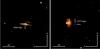 |
Fig. 1 Colour composite images in U, B, and V of SN 2013gh in NGC 7183 and iPTF 13dge in NGC 1762 obtained with NOT on Sep. 10 and Sep. 23, respectively. |
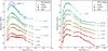 |
Fig. 2 Light curves of SN 2013gh (left) and iPTF 13dge (right). The data were obtained from Swift (stars), LCOGT (squares), and NOT (circles). For the V-band light curves we show the fitted splines that were used to obtain the colours as described in the text. For the remaining filter we also display fitted splines to guide the eye. However, these were never used in the analysis. |
The supernova 2013gh (Hayakawa et al. 2013), first designated as PSN J22022184-1855004, was discovered by the Lick Observatory Supernova Search (LOSS) with the Katzman Automatic Imaging Telescope (Filippenko et al. 2001) in images obtained on 2013 Aug. 6.4 (UT dates are used throughout this paper). The SN was subsequently classified as an underluminous and/or reddened SN Ia one week before maximum brightness by the Las Cumbres Observatory Global Telescope (LCOGT) with FLOYDS on Faulkes Telescope South on Aug. 11.6 (Sand et al. 2013). The supernova SN 2013gh is located in NGC 7183, a peculiar S0-type galaxy at redshift z = 0.0088 (Fisher et al. 1995). The proximity to an apparent dust lane of its host galaxy, visible in Fig. 1, suggests that the SN could be reddened and that ISM absorption lines may be present.
The discovery of iPTF 13dge in NGC 1762, at z = 0.0159 (Theureau et al. 1998), was made by the intermediate Palomar Transient Factory (iPTF) survey on Sep. 4.5 and classified as a SN Ia with the Low Resolution Imaging Spectrometer (LRIS) on the 10 m Keck-I telescope on Sep. 4.6 (Cao et al. 2013). The SN appears to be in the outer reaches of the host galaxy where no obvious dust lanes are visible, as can be seen in Fig. 1.
Here we present photometry obtained with LCOGT and with the Nordic Optical Telescope (NOT) using the 6.4′ × 6.4′ Andalucia Faint Object Spectrograph and Camera (ALFOSC) of both SNe as well as observations from the Ultraviolet/Optical Telescope (UVOT; Roming et al. 2005) on the Swift spacecraft (Gehrels et al. 2004) of SN 2013gh.
Standard reduction with bias subtraction and flat-field correction were applied to all the ground-based data. For the NOT data the SN flux was measured following the method outlined by Valenti et al. (2011) using point-spread function (PSF) photometry where the host background was simultaneously estimated by fitting a polynomial. For the LCOGT data, on the other hand, the photometry of SN 2013gh was obtained after reference images had been subtracted, with the exception of the U-band data where the flux was measured directly using PSF photometry. Similarly, the photometry for all bands of iPTF 13dge could be obtained using PSF photometry directly owing to the significant separation between the SN and the host. All ground-based photometry was calibrated using either Landolt standards or stellar photometry from the Sloan Digital Sky Survey. Furthermore, the UVOT photometry was obtained from the Swift Optical/Ultraviolet Supernova Archive (SOUSA; Brown et al. 2014). The reduction is based on that of Brown et al. (2009), including subtraction of the host-galaxy count rates, and uses the revised UV zeropoints and time-dependent sensitivity from Breeveld et al. (2011). All photometry is presented in Table 2 and the light curves are shown in Fig. 2.
Supernova coordinates quoted from the discovery telegrams.
Measured photometry of SN 2013gh and iPTF 13dge.
Having UV and optical photometry of SN 2013gh, we use the method outlined by Amanullah et al. (2015) to simultaneously fit the extinction-law parameters RV and E(B−V) together with the time of B-band maximum, tBmax, and the light-curve decline rate parametrised by the stretch parameter, s. The fit is based on the assumption that the observed colours of SN 2013gh can be described by the colours of the normal and unreddened SN 2011fe together with the Fitzpatrick (1999) extinction law. The colours of the two objects are further compared for the same effective light-curve-width-corrected “phases” p, which for each SN is defined as p = (t−tBmax)/(1 + z) /s, where t is time in the observer’s frame, z the redshift of the object, and tBmax and s are left as free parameters for SN 2013gh but kept fixed for SN 2011fe as described by Amanullah et al. (2015).
The observed colours were studied for each filter with respect to the V band, which could be obtained directly for the epochs where V observations were available. For the remaining epochs the V magnitudes were obtained from a fitted spline model to the existing data using SNooPy (Burns et al. 2011). SNooPy is a software package primarily designed to fit light-curve parameters of SNe Ia but can also be used to fit different models to the light-curve data. The V magnitudes that were used to measure the colours are also shown in Table 3, where column seven indicates whether the value was obtained from data or from the SNooPy model. In this table we have summarised all the data that were used to calculate the colours, and column four lists the measurements adopted from Table 2. We also calculate the Galactic extinction for each point using the values from Table 1 as well as the cross-filter corrections, KX, between the observed filters and the corresponding filter for which SN 2011fe has been observed. The details can be found in Amanullah et al. (2015).
The best-fit light curve and reddening-law parameters are shown in Table 4 using all data between phases −10 and + 35 days from tBmax. In Fig. 3, the RV vs. E(B−V) contours of the best fit are shown.
On the other hand, iPTF 13dge, had very low reddening which did not allow RV to be well constrained. For this SN we fit the reddening after fixing RV = 3.1.
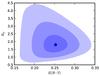 |
Fig. 3 Statistical confidence contours at the 68.3%, 95.5%, and 99.7% levels of the RV and E(B−V) fit to the SN 2013gh observed light-curve colours. The point shows the best-fit value from Table 4. See text for details. |
3. High-resolution spectroscopy
Three epochs of high-resolution spectra of SN 2013gh as well as one epoch of iPTF 13dge were obtained with the Ultraviolet and Visual Echelle Spectrograph (UVES; Dekker et al. 2000) on UT2 at the Very Large Telescope (VLT) of the European Southern Observatory (ESO). The REFLEX (ESOREX) reduction pipeline provided by ESO was used to reduce the raw UVES data. Another high-resolution spectrum of iPTF 13dge was obtained with the High Resolution Echelle Spectrograph (HIRES; Vogt et al. 1994) mounted on the Keck-I telescope. The HIRES spectrum was reduced using the XIDL reduction pipeline1. These high-resolution spectra along with estimated signal-to-noise ratio (S/N) and resolution are summarised in Table 5.
Photometry of SN 2013gh and iPTF 13dge.
We have used the line-modelling software Molecfit (Smette et al. 2015; Kausch et al. 2015) to correct for telluric features in relevant parts of the spectra.
Absorption features of spectra can be characterised by their equivalent widths (EWs), which can be measured using the point-to-point formula 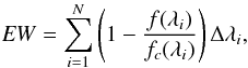 (1)where f and fc are the actual flux and continuum flux at a given wavelength λ, respectively. The propagated uncertainty, σEW, is given by
  (2)where σf is the uncertainty of the actual flux and σfc is the uncertainty of the continuum flux fc.
We have found that the REFLEX pipeline produces larger uncertainties than the root-mean-square (rms) scatter about the continua of spectra. Over short sections of the spectra, the rms scatter appears to be ~ 35% less than the average pipeline uncertainties. For this reason, we use the rms scatter instead of the pipeline output uncertainties to compute EWs.
The continuum near well-defined lines such as Na I D and Ca II H&K can be determined by fitting a third-degree polynomial to sections bracketing the features. This method works poorly for broad, diffuse features such as DIBs, since the features themselves are not easily separable from the continua. Therefore, we simultaneously fit a polynomial and a Gaussian function to determine the continuum with the polynomial parameters. The EWs of the DIBs can subsequently be computed using Eq. (1). We also fit multiple Voigt profiles using VPFIT2 to the absorption lines to determine individual components and column densities, where relevant.
Light-curve and reddening parameters of SN 2013gh and iPTF 13dge obtained by fitting the colour curves of SN 2011fe to the observed data together with the Fitzpatrick (1999) extinction model using the method outlined by Amanullah et al. (2015).
Obtained high-resolution spectra with stretch-corrected phases in the rest frame with respect to tBmax.
3.1. SN 2013gh
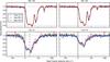 |
Fig. 4 Absorption line profiles of the Na I D doublet and Ca II H&K in the three UVES spectra of SN 2013gh. The spectra are normalised and the Sep. 24.0 spectrum is binned for clarity in the Ca II H&K subplots. The solid vertical lines indicate the rest-frame wavelength of the host galaxy NGC 7183 (according to the spectroscopic redshift in Fisher et al. 1995). The dashed vertical line in the Ca II K subplot indicates the Milky Way rest-frame wavelength of Ca II H. |
The spectra of SN 2013gh display the deep multiple-feature Na I D and Ca II H&K lines shown in Fig. 4. The redshifted wavelength of Ca II K nearly coincides with the rest-frame wavelength of Ca II H, causing the host-galaxy Ca II K and Milky Way Ca II H lines to blend. At the host-galaxy rest-frame wavelength we detect the DIBs listed in Table 6, of which the DIBs λλ5797, 6379, and 6614 are most clearly defined and plotted in Fig. 5. Unfortunately, the DIB λ5780, which was discussed as a reddening proxy by Phillips et al. (2013), falls into a gap not covered by the UVES spectra.
In Table 6 the measured EW values of all identifiable ISM species of SN 2013gh are presented. We use the relations of Poznanski et al. (2012) and Baron et al. (2015) to estimate E(B−V) from Na I D and the DIB λ5797, respectively. It can be seen that the line ratios Na I D2/D1 are < 2, implying that the Poznanski et al. (2012) relation gives at best a lower limit for E(B−V). Nevertheless, the E(B−V) limit alone places SN 2013gh into the group of SNe with unusually high Na I column densities as defined by Phillips et al. (2013). Furthermore, the value of E(B−V) can be estimated from the EW of DIBs using empirical relations (e.g. Baron et al. 2015). The DIB λ5797, for example, is roughly consistent with the measured E(B−V) from photometry. Interestingly, most of the DIBs are comparable within uncertainties to those detected in SN 2001el (Sollerman et al. 2005), a SN Ia that matches SN 2013gh in photometric reddening.
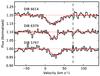 |
Fig. 5 Three DIBs of SN 2013gh with well-defined profiles. The spectra are normalised, binned, and offset from one another. The red solid lines are the best-fit Gaussian profiles of the features. The dashed vertical line indicates the velocity of the small feature at v ≈ 73 km s-1 in Na I D. |
Equivalent widths of Na I D, Ca II H&K, and the detectable DIBs in SN 2013gh.
As we can see in Figs. 4 and 5, that the typical ISM features appear to be redshifted with respect to the recession velocity of NGC 7183. Furthermore, the coordinates of the SN are consistent with a location in the redshifted arm in Very Large Array (VLA) H I data3. The deepest absorption features in both Na I D and Ca II H span velocities of v ≈ 10−30 km s-1. Another blended set of features appears redshifted from these at v ≈ 40 km s-1. Finally, a small, seemingly unblended feature appears at v ≈ 73 km s-1 in Na I D, but it is absent from Ca II H&K.
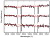 |
Fig. 6 The three spectra of SN 2013gh around the Na I D doublet, highlighting the possible diffuse feature of the profile (red solid line). The spectra have not been normalised, excluding the possibility that the broad feature is an artefact of the normalisation procedure. The dotted vertical lines indicate the rest-frame velocity of the host galaxy. |
On the blueshifted side of the Na I D profile, there appears to be a shallow diffuse feature or wing of a Voigt profile. In Fig. 6, we show the non-normalised spectra at the three epochs around the Na I D doublet. The broad feature can be visually identified at all three epochs and is thus not an artefact of the normalisation procedure. We find that the feature is not symmetric about the deepest features of the Na I D profile, indicating that it may be a broad diffuse component of the ISM. In Fig. 6, broad Gaussians with σvel ≈ 50 km s-1 are shown, which are centred on the rest-frame velocity of NGC 7183.
Interestingly, an H I spectrum extracted at the position of SN 2013gh exhibits emission which is centred on and spans approximately the same range as the broad feature. It is therefore possible that the broad feature corresponds to diffuse Na I gas tracing H I. If this is the case, then the broad feature corresponds to the warm ISM, unlike the deep Na I D absorption features which typically trace the cold ISM. Assuming that the broad feature traces H I gas, this could suggest that SN 2013gh is located on the far side of NGC 7183.
3.2. Varying Na I D feature
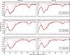 |
Fig. 7 Redshifted features of the Na I D profile of SN 2013gh along with the Voigt profiles obtained with VPFIT. The model telluric spectra of the respective epochs are plotted for reference above the continua. It can be seen that the feature at v ≈ 73 km s-1 probably changes in depth, whereas the other features only appear to change because of differences in the resolution of the spectra. |
Voigt profile parameters of the redshifted features of Na I D in SN 2013gh determined with VPFIT.
To search for line variations in SN 2013gh, we have measured the EWs of all features and compared the individual epochs. While DIBs and Ca II H&K appear not to change significantly, there is a slight decrease in the EW of Na I D. Guided by visual inspection, there appear to be differences between the individual epochs in the redshifted part of the Na I D profile. In Fig. 7, the profiles of the redshifted Na I D features of each epoch and the fitted Voigt profiles are shown. The positions of telluric lines can be inferred from the model telluric spectra plotted above the respective SN spectra.
The higher resolution of the first epoch is evident in the region v = 40−50 km s-1, where the troughs between individual components can be visually distinguished. Estimates of the resolution (R = λ/ Δλ) for each spectrum can be found in Table 5. We find that the feature at v = 35−60 km s-1 can be fit by three Voigt profiles. The EW in this velocity range does not change significantly between the individual epochs and the column densities of the individual components inferred from the Voigt profile fits do not show any significant variations either. The Voigt profile parameters of the best fit are summarised in Table 7. Since neither the column densities nor the total EW of the components at v = 35−60 km s-1 appear to vary, the visual differences between the individual epochs must be caused by differences in the resolution of the spectra.
The most redshifted feature at v ≈ 73 km s-1, however, does appear to vary between the epochs. It is important to ascertain that the variations are not an effect of changing telluric lines. First, the feature displays the same trend in both Na I D1 and D2, implying that telluric lines would need to overlap with both features to explain the change. Second, the depth of the telluric lines would have to change with the same trend as observed in the spectra. In Fig. 7, the model telluric spectra of the individual epochs are plotted to show the approximate locations of telluric lines with respect to the feature. No telluric lines appear to overlap with the feature in any of the epochs, nor is there an obvious trend in the depth of the telluric lines. Furthermore, we ascertained that the depth of the telluric lines in the standard-star spectra obtained on the same epochs do not display any trend either. Thus, poorly subtracted telluric lines are unlikely to account for the variations observed in the feature at v ≈ 73 km s-1.
We also checked that the changes are not an unusual systematic error, in which case other absorption features might display a similar trend. The other components of the Na I D doublet of the host galaxy are much deeper than the feature we would like to compare them to. However, the Milky Way Na I D doublet consists of three components of comparable depth to the changing feature. The EWs of these three Milky Way features show neither any significant variations between the epochs nor any trend. Lastly, individual exposures of the same epochs (see Fig. A.1) agree very well with each other, indicating that there are no systematic changes within a night. From the above we conclude that the reduced and normalised spectra can be trusted.
We have measured the EWs of the feature at v ≈ 73 km s-1 in each exposure. The measurements are presented in Appendix A, and we also convince ourselves that the decrease in measured EW is significant. This was done using a bootstrap analysis that indicates that the change in EW is inconsistent with random noise of a feature which does not vary with time.
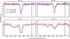 |
Fig. 8 Absorption line profiles of the Na I D doublet and Ca II H&K of iPTF 13dge obtained with UVES (Sep. 12.3) and HIRES (Sep. 16.5). The Ca II K&H lines have been binned for clarity. Cosmic rays in Na I D2 and Ca II K in the HIRES spectra have been masked. |
The Voigt profile fits further confirm the assertion that the v ≈ 73 km s-1 feature is changing. Interestingly, the Doppler broadening of the feature was found to be much more narrow than the observed profile with b = 0.8 ± 0.1 km s-1. Thus, the feature is unresolved, deeper than it appears, and in fact not optically thin. Visually, the varying feature appears to decrease only in depth and not in width, which is consistent with an unresolved line profile. In Table 7 the Na I column densities inferred from the Voigt profile fits are presented. The Doppler broadening (b) of the respective features were determined from the first epoch and fixed for the following epochs. The fits indicate that the column density of the v ≈ 73 km s-1 feature is decreasing with time, while the other features are not changing. Although the changing feature could also be explained by a decrease in intrinsic line width with unchanging column density, there is no obvious physical scenario in which this could be the case. Thus, the best explanation for the changes seen in the data is a decrease in column density.
To summarise, we have identified an Na I D component at v ≈ 73 km s-1 which appears to be varying with time. Telluric lines cannot account for the variations, since there are no telluric lines that overlap with the changing feature. Furthermore, there does not appear to be any reason to believe that the variations might be caused by some systematic effect. Individual exposures at the same epochs seem to be very consistent with one another and no other features show the same trend over time. The decreasing EW can be measured in all individual exposures of the three epochs, and a simple bootstrap test has shown that it is very unlikely to obtain this result from random noise. The Voigt profile fits further confirm that the column density of Na I is decreasing. Also, the fits demonstrate that the line is very narrow and the profile is in fact not resolved. We thus conclude that the variations seen in the feature are real and most likely produced by a decreasing column density of Na I atoms along the line of sight.
3.3. iPTF 13dge
The two high-resolution spectra obtained of iPTF 13dge were taken only four nights apart. However, the early epochs at which the spectra were taken make the interval sensitive to photoionisation as will be shown in Sect. 4.3. The HIRES spectrum is contaminated by many cosmic rays, affecting both the Na I D and Ca II H&K lines. The Na I D doublets as well as Ca II H&K of both spectra are shown in Fig. 8, though cosmic rays were masked in the HIRES spectrum. Interestingly, the Ca II lines appear to have an additional blueshifted feature that is not visible in the Na I D doublet. No DIBs could be identified in either spectra. The EW values of the detected features are given in Table 8 along with E(B−V) estimates using the Poznanski et al. (2012) relation. The Na I D2/D1 line ratio clearly shows that the lines are not optically thin. This in turn implies that the E(B−V) estimates are merely lower limits. Although the value is in good agreement with the E(B−V) presented in Table 4, one must keep in mind that the photometric value has been computed with a fixed RV = 3.1.
Comparing the absorption lines of both epochs has not revealed any significant variations. The Ca II H&K EWs are consistent with one another within the uncertainties. We inspected the Na I D doublet in more detail, because there seems to be a slight difference between the epochs in Na I D2. While the EW of Na I D2 does not change between the epochs, there appears to be a 2σ decrease in EW in Na I D1. Since this could be consistent with a decreasing feature in the nonlinear part of the curve of growth, we fit Voigt profiles to the features to determine the Na I column densities. The Na I D profile is consistent with two components, the parameters of which are presented in Table 9. Unfortunately, the column densities obtained from the Voigt profiles do not change significantly. Thus, no definite change could be detected in any absorption feature of iPTF 13dge.
Equivalent widths of Na I D and Ca II H&K of iPTF 13dge.
Voigt profile parameters of Na I D in iPTF 13dge determined with VPFIT.
4. Interpretation of varying absorption lines
In Sect. 3.2, we saw that the small redshifted feature of the Na I D doublet of SN 2013gh varies over time. There are several possibilities by which this could occur. The first two we consider are geometric effects caused by either rapidly moving or patchy clouds along the line of sight. Another possibility is that photoionisation produced by the UV flux of the SN decreases the column density of an absorber.
4.1. Geometric effects
A variety of geometric effects could give rise to varying column densities of absorbers. Unfortunately, the varying Na I D feature is not detected in the profiles of any other ISM species for comparison. The absence of the feature in Ca II H&K suggests that there is very little Ca II in the cloud or it is locked up in dust grains. Thus, it is not possible to use Ca II H&K to test for a geometric origin of the variations seen in Na I D.
One geometric effect we considered is that the small feature corresponds to a gas cloud passing through the line of sight to the SN. To observe variations on the timescale of weeks, a gas cloud must have column density variations on small scales and be moving at a high velocity. The size of the column density variations and the velocity of the cloud are inversely proportional. For instance, one could suppose that the small varying feature has a transverse velocity of the same order of magnitude (vtrans ≈ 100 km s-1) as the line-of-sight velocity with respect to the galaxy rest frame. To then see variations on the order of tens of days, the gas cloud must have a diameter of scale Rtrans ≈ 1 AU.
A second possibility is that an unchanging gas cloud is close enough to the SN for there to be a projection effect on the expanding photosphere (Patat et al. 2010). The scenario is possible if, for example, a small gas cloud initially overlaps with the entire photosphere, but later is too small to veil the expanded photosphere. The method is restricted to detecting column density variations in gas clouds that are smaller in scale than the size of the photosphere. Assuming a spherical gas cloud with homogeneous volume density and centred on the photosphere, the variations in Na I D of SN 2013gh are consistent with a cloud having a radius Rproj ≈ 220 AU. This would imply that the true geometry of the gas cloud must vary on scales smaller than Rproj.
The two geometric effects considered above could be the origin of the variations detected in Na I D. However, this could only be confirmed if the corresponding absorption feature were detected in another absorption profile and displayed exactly the same trend in column density over time. As in the case of SN 2006X, a geometric origin of the Na I D variations in SN 2013gh cannot be ruled out (Patat et al. 2007).
4.2. Photoionisation
Another possible source of absorption-line variations is by photoionisation of the gas by UV radiation from the SN. Knowing the UV flux of a SN and the ionisation cross-section of an absorber, the ionisation rate at a given distance from the SN and at a given phase can be modelled (Borkowski et al. 2009).
The biggest uncertainty in the model is the UV flux of the SN itself. In particular, only a few SNe have had UV spectra taken at early phases. Furthermore, it is known that the largest differences between individual SNe occur in the UV part of the spectrum (see, e.g. Brown et al. 2010). This becomes apparent when comparing the commonly used templates of Hsiao et al. (2007, hereafter H07) and SN 2011fe (e.g. Amanullah et al. 2015). Below ~ 2400 Å, the ionisation energy of Na I (via NIST; Kramida et al. 2014), the peak flux of the H07 template is a factor of ~ 4 greater than that of SN 2011fe.
Motivated by the excellent UV coverage and low extinction of SN 2011fe, we used the spectral energy distribution (SED) described by Amanullah et al. (2015) to compute the photoionisation rates. However, the H07 template extends to both shorter wavelengths and earlier phases than the SN 2011fe template. We therefore extrapolated the SN 2011fe SED by that of H07, which was scaled to match the flux at the “edges” of the SN 2011fe template at 1750 Å. Furthermore, the early phases of the H07 template were scaled by a factor determined from the earliest SN 2011fe spectrum.
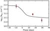 |
Fig. 9 The best-fit photoionisation curve for the varying Na I D feature in SN 2013gh. |
Using the extrapolated SED and wavelength-dependent ionisation cross-sections (Verner et al. 1996)4, we can model the photoionisation of an absorber. Assuming that the gas is optically thin and situated in a thin shell, the ionisation rate is characteristic for the radius of the shell. Therefore, we can fit the model to the column-density data obtained from the changing Na I D feature of SN 2013gh to determine the initial column density of the gas and the distance from the SN. In Fig. 9, the best-fit photoionisation curve is plotted along with the Na I column-density measurements of the varying feature. For the best fit, we find that the initial column density must have been log 10 { NNa I (cm-2) } = 11.38 ± 0.02 at a distance log 10 { Rion (cm)} = 18.9 ± 0.2, where the uncertainties incorporate a range of total ionising flux of ± 1 mag, to crudely estimate the effects of different UV brightness.
We have independently verified the photoionisation result with an ionisation and excitation code used to study absorption-line variability in gamma-ray burst afterglow environments from Vreeswijk et al. (2013). The resulting radius log 10 { Rion (cm)} = 18.89 ± 0.04 and initial column density log 10 { NNa I (cm-2) } = 11.38 ± 0.04 are in excellent agreement with the above results. The smaller uncertainty in the distance does not take into account the possible range of flux of the SED.
Since we consider photoionisation as a possible cause for the observed line variation, we would like to argue why recombination is not relevant on the timescale of the observations. Following a similar a argument as by Simon et al. (2009), the recombination timescale is  (3)where α is a rate coefficient for a given temperature and ne is the volume density of electrons. Since the properties of the varying cloud are not known, we will determine a conservative value of ne for a recombination timescale which would affect the above results. Assuming a typical ISM cloud temperature of ~ 102 K (Glassgold et al. 2012), the rate coefficient for Na I is α ≈ 10-11 cm3 s-1 (Badnell 2006). Note that this assumption is conservative; the recombination time will increase with greater temperature, if the gas is heated by the SN or progenitor. Recombination would need to be taken into account if the recombination timescale is ~ 10 days or τrec ≈ 106 s. This would imply an electron density ne ≈ 105 cm-3. Chugai (2008) uses this ne value for electrons streaming from an SD progenitor at ~ 1017 cm from the SN. At greater distances, however, the electron density should drop off, at 1019 cm being much lower than the limit computed. Thus, recombination should be negligible in the case of the varying Na I D feature, or else the ionisation rate is underestimated by the simple photoionisation model.
4.3. Absorbers in the CS environment
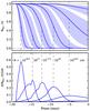 |
Fig. 10 Photoionisation fraction of Na I and rate as a function of phase at distances between 1016.5 and 1018.5 cm from a SN. The dashed vertical lines associate the curves of the two plots with one another and are labeled by their respective radii at which the gas is situated from the explosion. The shaded bands indicate the ± 1 mag change in ionising UV flux from the SN. The Na I gas is assumed to be optically thin and is completely ionised at all radii considered in this plot. |
The photoionisation rate is a function of the shell radius of an absorber and of the time after the explosion. In Fig. 10, the time-dependent photoionisation of Na I gas of shells at radii ranging from 1016.5 to 1018.5 cm are considered. The upper plot shows the fractional decrease of Na I with time with respect to the initial column density. In the lower plot the rate of photoionisation of the respective gas shells is shown. To probe for photoionisation at a given radius from the SN it is thus necessary to obtain spectra spanning the time during which there is a significant rate of photoionisation. For instance, one must obtain spectra before ~ 8 days prior to maximum light to probe radii of < 1018 cm using Na I absorption. The exact phase at which the maximum rate of photoionisation occurs depends on the UV luminosity of the SN. The brighter a SN is in UV radiation, the earlier ionisation will occur. In Fig. 10, the shaded bands show the range of ionisation curves if the brightness is varied by ± 1 mag. The model does not take into account recombination (see Sect. 4.2), preionisation by the progenitor system or shock-breakout UV flash (Cumming et al. 1996), which could ionise the innermost radii from the SNe.
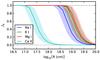 |
Fig. 11 Total fraction of photoionisation of different ISM species as a function of distance from the SN. The bands indicate a ± 1 mag change in ionising UV flux. |
From the absence of absorption-line variations, the photoionisation model can also be used to exclude radii at which the absorber is located from the SN. Even though the high-resolution spectra of iPTF 13dge were taken only four days apart, it can be seen in Fig. 10 that significant ionisation can occur during these phases. Between −9 and −5 days before maximum brightness, the photoionisation model is sensitive to ionisation occurring at distances of 6 × 10¹⁷−5 × 1018 cm from the SN, whereby the possible range in UV brightness is not taken into account. It thus indicates that the visible Na I D features are not located at these radii.
So far the search for varying absorption lines has mainly focused on the Na I D doublet. This is motivated by the fact that it is relatively easy to obtain high-S/N spectra around the wavelength of Na I D. Being a doublet furthermore helps to ascertain whether variations in Na I D are real, when they are detected in both profiles. The recent example of varying K I lines in SN 2014J (Graham et al. 2015) has shown that it is not necessary to solely focus on Na I D. We therefore investigated some other typical ISM species.
In addition to Na I, we have investigated the photoionisation of the absorbers in Table 10 more closely. While the ionising fluxes of Na I, K I, and Mg I are comparable, that of Ca II is roughly two orders of magnitude lower. The SED used does not cover wavelengths < 1000 Å, implying that some ionising flux is not taken into consideration. The SED cutoff is inadvertently close to the ionisation energy of H I at 911 Å, beyond which the H I gas likely shields all other particles from ionising flux. Judging by the rapid drop in flux at higher energies, the flux beyond the cutoff would only contribute a few percent to the total ionising flux of Na I, K I, and Mg I. Unfortunately, the ionisation energy of Ca II at 1044 Å is close to the cutoff, and thus the total ionising flux is underestimated. Assuming a roughly constant continuum in the range 911−1044 Å, the ionising flux of Ca II could be a factor of approximately three greater than the flux computed from the SED. Hence, the details of the ionising effects on Ca II must be taken with skepticism, but are presented below since they show that photoionisation of Ca II can occur around SNe Ia.
In Fig. 11, the final ionisation fraction as a function of radius is shown for the different absorbers. While the total ionisation of Na I, Mg I, and K I drop off at similar radii around ~ 1019 cm, Ca II is not ionised beyond a radius of ~ 1018 cm owing to the high ionisation energy. Figure 12 shows which radii are probed for photoionisation by taking spectra at different phases. From Fig. 12, one can infer to which radii the observations presented in this paper were sensitive. The large time interval between the first and second epoch of SN 2013gh spectra implies that a large range of radii 1017.5−1019.5 cm has been probed with Na I. The short interval between the two iPTF 13dge epochs, on the other hand, implies that the smaller range of radii 1018−1018.5 cm has been probed. Although similar limits could be set using Ca II, the uncertainty of the UV flux beyond the reaches of the SED would probably make them unreliable.
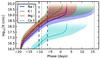 |
Fig. 12 Phases at which photoionisation occurs for different ISM species as a function of radius. The lines correspond to the peak ionisation rate, and the shaded region indicates the phases between which 80% of photoionisation occurs. The fading corresponds to the limit where < 5% of the gas is ionised in total. The ± 1 mag range of the ionising flux is not considered in this plot. The phases of the spectra taken of SN 2013gh (dotted lines) and iPTF 13dge (dashed lines) indicate which radii are probed for photoionisation. |
Ionisation energies and cross-sections of some typical ISM species.
5. Summary and conclusions
Our high-resolution spectra of the SN 2013gh and iPTF 13dge can be added to the slowly growing sample of narrow absorption line temporal series of SNe Ia.
The supernova SN 2013gh is reddened, and has negligible Galactic extinction (E(B−V)MW = 0.025 mag) and with a line of sight close to a dust lane in the host galaxy NGC 7183. Comparison of the Na I D and H I profiles indicates that SN 2013gh likely occurred on the far side of its host, indicating that the reddening is mainly due to dust in the host galaxy.
The time series of Na I D absorption has revealed a small redshifted feature with decreasing column density. Although the change is consistent with photoionisation occurring at ~ 1019 cm from the explosion, geometric effects cannot be excluded since the feature is not discernible in any other absorption-line profile. The time-varying component is unusual in that it is the most redshifted feature in the Na I D profile. If the feature is associated with outflowing gas from the progenitor, the SN could be located in a part of the host galaxy that is receding faster than the main absorption lines. However, the gas could also be unrelated to the SN and moving toward it. Unfortunately, the crowded line of sight close to the core of NGC 7183 and the proximity to a dust lane make a more definite determination of the origin of the varying Na I D feature in SN 2013gh difficult.
The temporal coverage of the spectra we have analysed should be sensitive to photoionisation of Na I gas occurring 1017.5−1019.5 cm from the SN, thus probing radii that can be considered part of the CS environment. The nondetections of further time-varying absorption features indicate that the high Na I column density in the SN 2013gh spectra does not originate from gas in these regions. Within 1017.5 cm, all Na I gas would have been ionised before the first spectrum was taken. Thus, it appears that the bulk of the gas must be situated in the ISM beyond 1019.5 cm from the SN. Compared to the reddening, the column density of Na I gas also appears to be unusually high with respect to the Poznanski et al. (2012) relation.
It should also be possible to exclude the presence of Ca II gas at even smaller radii (around 1017 cm) from the SN. However, given the small range of wavelengths covered by the SED above the ionising energy of Ca II, the exclusion range could shift. Nevertheless, the closely matching profiles of Ca II H and Na I D indicate that the two gases have the same distribution in the ISM.
Assuming that Na I and Ca II trace CS dust, the nondetections of varying absorption lines exclude a large range of radii from the explosion where dust could have been situated. Importantly, the earliest spectrum allowed us to probe for dust within ~ 1018 cm. Thus, we have been able to test regions where dust can have a significant effect on the light curve and observed RV of a SN (Amanullah & Goobar 2011; Goobar 2008).
With the two spectra of iPTF 13dge, we have only been able to test a narrow range of radii for photoionisation. The nondetection of variations in Na I D indicate that the gas is situated farther than 1018.5 cm from the explosion. Hence, in this case the Na I gas is also not located in the CS environment. The intriguing blueshifted feature in the Ca II H&K profiles which is entirely absent in Na I D raises the speculative possibility that a corresponding Na I D feature has already been fully ionised. If we trust the computed photoionisation curves of Ca II, this could have occurred in a sweet spot around ~ 1017.5 cm from the explosion. In the absence of an earlier spectrum where the hypothetical Na I D feature could still be present, or a later spectrum where the Ca II H&K feature could be partially ionised, this interpretation remains speculative.
We have seen that it is possible to constrain the presence of gas in the CS environment of SNe Ia by searching for variations in their absorption profiles due to photoionisation at early phases. The SED of SNe Ia indicates that gases such as Na I, K I, and Mg I within a radius of 1018 cm will entirely ionise before SN maximum brightness. Ca II would probably ionise slightly later, if at all, within these radii. In the search for varying absorption lines, spectral time series have so far mostly been taken after SN maximum brightness (e.g. Sternberg et al. 2014). At these phases, gases in the CS environment will been entirely ionised, reducing the observations to be sensitive to absorption-line variations caused only by recombination. Lastly, SNe with lines of sight that are clear of obvious dust lanes and far from their host-galaxy cores should be preferred in order to reduce effects originating from ISM gas and dust. To detect photoionisation effects on CS gases in the future, it is necessary to sample isolated SNe Ia with high-resolution spectra at early phases. Specifically, a high-resolution spectrum earlier than approximately eight days before maximum is required to probe regions within 1018 cm from SNe using Na I D absorption.
Obtained via phidrates.space.swri.edu
Acknowledgments
We would like to thank Alexis Brandeker for assisting us with the UVES data, Jesper Sollerman for his helpful comments, and Daniela Vergani for sharing graphs of the VLA H I data. R.A. and A.G. acknowledge support from the Swedish Research Council and the Swedish Space Board. The Oskar Klein Centre is funded by the Swedish Research Council. A.V.F.’s research was funded by US NSF grant AST-1211916, the TABASGO Foundation, and the Christopher R. Redlich Fund.
This work is based on observations collected at the European Organisation for Astronomical Research in the Southern Hemisphere under ESO programme 091.D-0352(A). We made use of Swift/UVOT data reduced by P. J. Brown and released in the Swift Optical/Ultraviolet Supernova Archive (SOUSA). SOUSA is supported by NASA’s Astrophysics Data Analysis Program through grant NNX13AF35G. This work is based on observations made with the Nordic Optical Telescope, operated by the Nordic Optical Telescope Scientific Association at the Observatorio del Roque de los Muchachos, La Palma, Spain, of the Instituto de Astrofisica de Canarias. The data presented here were obtained in part with ALFOSC, which is provided by the Instituto de Astrofisica de Andalucia (IAA) under a joint agreement with the University of Copenhagen and NOTSA. This work makes use of observations from the LCOGT network. Some of the data presented herein were obtained at the W. M. Keck Observatory, which is operated as a scientific partnership among the California Institute of Technology, the University of California, and NASA; the Observatory was made possible by the generous financial support of the W. M. Keck Foundation. The authors wish to recognise and acknowledge the very significant cultural role and reverence that the summit of Mauna Kea has always had within the indigenous Hawaiian community; we are most fortunate to have the opportunity to conduct observations from this mountain. This research used resources of the National Energy Research Scientific Computing Center, a DOE Office of Science User Facility supported by the Office of Science of the US Department of Energy under Contract No. DE-AC02-05CH11231. LANL participation in iPTF was funded by the US Department of Energy as part of the Laboratory Directed Research and Development program. A portion of this work was carried out at the Jet Propulsion Laboratory, California Institute of Technology, under contract with the National Aeronautics and Space Administration.
References
- Amanullah, R., & Goobar, A. 2011, ApJ, 735, 20 [NASA ADS] [CrossRef] [Google Scholar]
- Amanullah, R., Goobar, A., Johansson, J., et al. 2014, ApJ, 788, L21 [NASA ADS] [CrossRef] [Google Scholar]
- Amanullah, R., Johansson, J., Goobar, A., et al. 2015, MNRAS, 453, 3300 [NASA ADS] [CrossRef] [Google Scholar]
- Badnell, N. R. 2006, ApJS, 167, 334 [NASA ADS] [CrossRef] [Google Scholar]
- Baron, D., Poznanski, D., Watson, D., Yao, Y., & Prochaska, J. X. 2015, MNRAS, 447, 545 [NASA ADS] [CrossRef] [Google Scholar]
- Blondin, S., Prieto, J. L., Patat, F., et al. 2009, ApJ, 693, 207 [NASA ADS] [CrossRef] [Google Scholar]
- Borkowski, K. J., Blondin, J. M., & Reynolds, S. P. 2009, ApJ, 699, L64 [NASA ADS] [CrossRef] [Google Scholar]
- Breeveld, A. A., Landsman, W., Holland, S. T., et al. 2011, in AIP Conf. Ser. 1358, eds. J. E. McEnery, J. L. Racusin, & N. Gehrels, 373 [Google Scholar]
- Brown, P. J., Holland, S. T., Immler, S., et al. 2009, AJ, 137, 4517 [NASA ADS] [CrossRef] [Google Scholar]
- Brown, P. J., Roming, P. W. A., Milne, P., et al. 2010, ApJ, 721, 1608 [NASA ADS] [CrossRef] [Google Scholar]
- Brown, P. J., Breeveld, A. A., Holland, S., Kuin, P., & Pritchard, T. 2014, Ap&SS, 354, 89 [NASA ADS] [CrossRef] [Google Scholar]
- Brown, P. J., Smitka, M. T., Wang, L., et al. 2015, ApJ, 805, 74 [NASA ADS] [CrossRef] [Google Scholar]
- Burns, C. R., Stritzinger, M., Phillips, M. M., et al. 2011, AJ, 141, 19 [NASA ADS] [CrossRef] [Google Scholar]
- Cao, Y., Sesar, B., Perley, D., et al. 2013, ATel, 5366, 1 [NASA ADS] [Google Scholar]
- Chomiuk, L., Soderberg, A. M., Chevalier, R. A., et al. 2016, ApJ, 821, 119 [NASA ADS] [CrossRef] [Google Scholar]
- Chugai, N. N. 2008, Astron. Lett., 34, 389 [NASA ADS] [CrossRef] [Google Scholar]
- Crotts, A. P. S. 2015, ApJ, 804, L37 [NASA ADS] [CrossRef] [Google Scholar]
- Cumming, R. J., Lundqvist, P., Smith, L. J., Pettini, M., & King, D. L. 1996, MNRAS, 283, 1355 [NASA ADS] [CrossRef] [Google Scholar]
- Dekker, H., D’Odorico, S., Kaufer, A., Delabre, B., & Kotzlowski, H. 2000, in Optical and IR Telescope Instrumentation and Detectors, eds. M. Iye, & A. F. Moorwood, SPIE Conf. Ser., 4008, 534 [Google Scholar]
- Dilday, B., Howell, D. A., Cenko, S. B., et al. 2012, Science, 337, 942 [NASA ADS] [CrossRef] [Google Scholar]
- Filippenko, A. V., Li, W. D., Treffers, R. R., & Modjaz, M. 2001, in IAU Colloq. 183: Small Telescope Astronomy on Global Scales, eds. B. Paczynski, W.-P. Chen, & C. Lemme, ASP Conf. Ser., 246, 121 [Google Scholar]
- Fisher, K. B., Huchra, J. P., Strauss, M. A., et al. 1995, ApJS, 100, 69 [NASA ADS] [CrossRef] [Google Scholar]
- Fitzpatrick, E. L. 1999, PASP, 111, 63 [NASA ADS] [CrossRef] [Google Scholar]
- Foley, R. J., Fox, O. D., McCully, C., et al. 2014, MNRAS, 443, 2887 [NASA ADS] [CrossRef] [Google Scholar]
- Gehrels, N., Chincarini, G., Giommi, P., et al. 2004, ApJ, 611, 1005 [NASA ADS] [CrossRef] [Google Scholar]
- Glassgold, A. E., Galli, D., & Padovani, M. 2012, ApJ, 756, 157 [NASA ADS] [CrossRef] [Google Scholar]
- Goobar, A. 2008, ApJ, 686, L103 [NASA ADS] [CrossRef] [Google Scholar]
- Goobar, A., & Leibundgut, B. 2011, Ann. Rev. Nucl. Part. Sci., 61, 251 [NASA ADS] [CrossRef] [Google Scholar]
- Goobar, A., Johansson, J., Amanullah, R., et al. 2014, ApJ, 784, L12 [NASA ADS] [CrossRef] [Google Scholar]
- Graham, M. L., Valenti, S., Fulton, B. J., et al. 2015, ApJ, 801, 136 [NASA ADS] [CrossRef] [Google Scholar]
- Hayakawa, K., Cenko, S. B., Zheng, W., et al. 2013, Central Bureau Electronic Telegrams, 3706, 1 [NASA ADS] [Google Scholar]
- Hsiao, E. Y., Conley, A., Howell, D. A., et al. 2007, ApJ, 663, 1187 [NASA ADS] [CrossRef] [Google Scholar]
- Iben, Jr., I., & Tutukov, A. V. 1984, ApJS, 54, 335 [NASA ADS] [CrossRef] [Google Scholar]
- Johansson, J., Amanullah, R., & Goobar, A. 2013, MNRAS, 431, L43 [NASA ADS] [CrossRef] [Google Scholar]
- Johansson, J., Goobar, A., Kasliwal, M. M., et al. 2016, MNRAS, submitted [arXiv:1411.3332] [Google Scholar]
- Kausch, W., Noll, S., Smette, A., et al. 2015, A&A, 576, A78 [NASA ADS] [CrossRef] [EDP Sciences] [Google Scholar]
- Kramida, A., Ralchenko, Y., J., R., & NIST ASD Team 2014, NIST Atomic Spectra Database, ver. 5.2, http://physics.nist.gov/asd [Google Scholar]
- Maeda, K., Tajitsu, A., Kawabata, K. S., et al. 2016, ApJ, 816, 57 [NASA ADS] [CrossRef] [Google Scholar]
- Maguire, K., Sullivan, M., Patat, F., et al. 2013, MNRAS, 436, 222 [NASA ADS] [CrossRef] [Google Scholar]
- Margutti, R., Parrent, J., Kamble, A., et al. 2014, ApJ, 790, 52 [NASA ADS] [CrossRef] [Google Scholar]
- Marion, G. H., Brown, P. J., Vinkó, J., et al. 2016, ApJ, 820, 92 [NASA ADS] [CrossRef] [Google Scholar]
- Munari, U., & Zwitter, T. 1997, A&A, 318, 269 [NASA ADS] [Google Scholar]
- Nugent, P. E., Sullivan, M., Cenko, S. B., et al. 2011, Nature, 480, 344 [NASA ADS] [CrossRef] [Google Scholar]
- Panagia, N., Van Dyk, S. D., Weiler, K. W., et al. 2006, ApJ, 646, 369 [NASA ADS] [CrossRef] [Google Scholar]
- Patat, F., Chandra, P., Chevalier, R., et al. 2007, Science, 317, 924 [NASA ADS] [CrossRef] [EDP Sciences] [PubMed] [Google Scholar]
- Patat, F., Cox, N. L. J., Parrent, J., & Branch, D. 2010, A&A, 514, A78 [NASA ADS] [CrossRef] [EDP Sciences] [Google Scholar]
- Patat, F., Taubenberger, S., Cox, N. L. J., et al. 2015, A&A, 577, A53 [NASA ADS] [CrossRef] [EDP Sciences] [Google Scholar]
- Phillips, M. M., Simon, J. D., Morrell, N., et al. 2013, ApJ, 779, 38 [NASA ADS] [CrossRef] [Google Scholar]
- Poznanski, D., Prochaska, J. X., & Bloom, J. S. 2012, MNRAS, 426, 1465 [NASA ADS] [CrossRef] [Google Scholar]
- Raskin, C., & Kasen, D. 2013, ApJ, 772, 1 [NASA ADS] [CrossRef] [Google Scholar]
- Ritchey, A. M., Welty, D. E., Dahlstrom, J. A., & York, D. G. 2015, ApJ, 799, 197 [NASA ADS] [CrossRef] [Google Scholar]
- Roming, P. W. A., Kennedy, T. E., Mason, K. O., et al. 2005, Space Sci. Rev., 120, 95 [NASA ADS] [CrossRef] [Google Scholar]
- Sand, D., Valenti, S., Howell, D. A., & Graham, M. 2013, ATel, 5262, 1 [NASA ADS] [Google Scholar]
- Schlafly, E. F., & Finkbeiner, D. P. 2011, ApJ, 737, 103 [NASA ADS] [CrossRef] [Google Scholar]
- Schlegel, D. J., Finkbeiner, D. P., & Davis, M. 1998, ApJ, 500, 525 [NASA ADS] [CrossRef] [Google Scholar]
- Shen, K. J., Guillochon, J., & Foley, R. J. 2013, ApJ, 770, L35 [NASA ADS] [CrossRef] [Google Scholar]
- Simon, J. D., Gal-Yam, A., Gnat, O., et al. 2009, ApJ, 702, 1157 [NASA ADS] [CrossRef] [Google Scholar]
- Smette, A., Sana, H., Noll, S., et al. 2015, A&A, 576, A77 [NASA ADS] [CrossRef] [EDP Sciences] [Google Scholar]
- Sollerman, J., Cox, N., Mattila, S., et al. 2005, A&A, 429, 559 [NASA ADS] [CrossRef] [EDP Sciences] [Google Scholar]
- Sternberg, A., Gal-Yam, A., Simon, J. D., et al. 2011, Science, 333, 856 [NASA ADS] [CrossRef] [Google Scholar]
- Sternberg, A., Gal-Yam, A., Simon, J. D., et al. 2014, MNRAS, 443, 1849 [NASA ADS] [CrossRef] [Google Scholar]
- Theureau, G., Bottinelli, L., Coudreau-Durand, N., et al. 1998, A&AS, 130, 333 [Google Scholar]
- Valenti, S., Fraser, M., Benetti, S., et al. 2011, MNRAS, 416, 3138 [NASA ADS] [CrossRef] [Google Scholar]
- Verner, D. A., Ferland, G. J., Korista, K. T., & Yakovlev, D. G. 1996, ApJ, 465, 487 [NASA ADS] [CrossRef] [Google Scholar]
- Vogt, S. S., Allen, S. L., Bigelow, B. C., et al. 1994, in Instrumentation in Astronomy VIII, eds. D. L. Crawford, & E. R. Craine, SPIE Conf. Ser., 2198, 362 [Google Scholar]
- Vreeswijk, P. M., Ledoux, C., Raassen, A. J. J., et al. 2013, A&A, 549, A22 [NASA ADS] [CrossRef] [EDP Sciences] [Google Scholar]
- Wang, X., Li, W., Filippenko, A. V., et al. 2008, ApJ, 677, 1060 [NASA ADS] [CrossRef] [Google Scholar]
- Webbink, R. F. 1984, ApJ, 277, 355 [NASA ADS] [CrossRef] [Google Scholar]
- Whelan, J., & Iben, Jr., I. 1973, ApJ, 186, 1007 [NASA ADS] [CrossRef] [Google Scholar]
Appendix A: Bootstrap
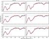 |
Fig. A.1 Comparison of all exposures of the redshifted Na I D profile of SN 2013gh. Exposures made at the same epochs are in good agreement with each other. |
To convince ourselves that the change detected with the Na I D Voigt profile fits of SN 2013gh is real (see Sect. 3.2), one should be able to confirm the result from the EW measurements alone. First, the absence of significant differences between exposures at the same epochs (see Fig. A.1) should reassure us that the measured changes are real and not caused by spurious fluctuations. The EWs of the v ≈ 73 km s-1 feature measured from all exposures can be found in Table A.1.
Since the change in EW of the redshifted Na I D feature of SN 2013gh is small, we would like to ascertain that the decrease is significant. We tested the significance with a bootstrap method constraining the likelihood of obtaining the result from random noise. For this we modelled the feature using the profile parameters obtained from the Voigt profile fit of the weighted averaged spectrum of all exposures. To the model absorption profiles, we added normal noise according to the S/N measured for the respective epochs. Next, we measured the resulting EWs of the features in the mock spectra. With the null hypothesis that the EW is not changing between the epochs, we fit a linear function to the combined equivalent width (Na I D1+D2) versus time. Finally, we determined the distribution of slopes obtained from the
mock data to compare with the slope of the real measurements. Figure A.2 shows the distribution of slopes of 105 mock spectra. The vertical solid line marks the slope of the linear fit to the real observed data, which is ~ 5σ from the distribution mean. This suggest that the variations cannot be the result of random noise.
Measured EWs of all exposures of the feature at v ≈ 73 km s-1 in SN 2013gh.
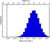 |
Fig. A.2 Distribution of slopes obtained by fitting a linear function to the combined equivalent width (D1+D2) values of 105 mock sets of spectra. The solid vertical line indicates the slope of the linear fit to the real data. |
All Tables
Light-curve and reddening parameters of SN 2013gh and iPTF 13dge obtained by fitting the colour curves of SN 2011fe to the observed data together with the Fitzpatrick (1999) extinction model using the method outlined by Amanullah et al. (2015).
Obtained high-resolution spectra with stretch-corrected phases in the rest frame with respect to tBmax.
Voigt profile parameters of the redshifted features of Na I D in SN 2013gh determined with VPFIT.
All Figures
|
Fig. 1 Colour composite images in U, B, and V of SN 2013gh in NGC 7183 and iPTF 13dge in NGC 1762 obtained with NOT on Sep. 10 and Sep. 23, respectively. |
| In the text | |
|
Fig. 2 Light curves of SN 2013gh (left) and iPTF 13dge (right). The data were obtained from Swift (stars), LCOGT (squares), and NOT (circles). For the V-band light curves we show the fitted splines that were used to obtain the colours as described in the text. For the remaining filter we also display fitted splines to guide the eye. However, these were never used in the analysis. |
| In the text | |
|
Fig. 3 Statistical confidence contours at the 68.3%, 95.5%, and 99.7% levels of the RV and E(B−V) fit to the SN 2013gh observed light-curve colours. The point shows the best-fit value from Table 4. See text for details. |
| In the text | |
|
Fig. 4 Absorption line profiles of the Na I D doublet and Ca II H&K in the three UVES spectra of SN 2013gh. The spectra are normalised and the Sep. 24.0 spectrum is binned for clarity in the Ca II H&K subplots. The solid vertical lines indicate the rest-frame wavelength of the host galaxy NGC 7183 (according to the spectroscopic redshift in Fisher et al. 1995). The dashed vertical line in the Ca II K subplot indicates the Milky Way rest-frame wavelength of Ca II H. |
| In the text | |
|
Fig. 5 Three DIBs of SN 2013gh with well-defined profiles. The spectra are normalised, binned, and offset from one another. The red solid lines are the best-fit Gaussian profiles of the features. The dashed vertical line indicates the velocity of the small feature at v ≈ 73 km s-1 in Na I D. |
| In the text | |
|
Fig. 6 The three spectra of SN 2013gh around the Na I D doublet, highlighting the possible diffuse feature of the profile (red solid line). The spectra have not been normalised, excluding the possibility that the broad feature is an artefact of the normalisation procedure. The dotted vertical lines indicate the rest-frame velocity of the host galaxy. |
| In the text | |
|
Fig. 7 Redshifted features of the Na I D profile of SN 2013gh along with the Voigt profiles obtained with VPFIT. The model telluric spectra of the respective epochs are plotted for reference above the continua. It can be seen that the feature at v ≈ 73 km s-1 probably changes in depth, whereas the other features only appear to change because of differences in the resolution of the spectra. |
| In the text | |
|
Fig. 8 Absorption line profiles of the Na I D doublet and Ca II H&K of iPTF 13dge obtained with UVES (Sep. 12.3) and HIRES (Sep. 16.5). The Ca II K&H lines have been binned for clarity. Cosmic rays in Na I D2 and Ca II K in the HIRES spectra have been masked. |
| In the text | |
|
Fig. 9 The best-fit photoionisation curve for the varying Na I D feature in SN 2013gh. |
| In the text | |
|
Fig. 10 Photoionisation fraction of Na I and rate as a function of phase at distances between 1016.5 and 1018.5 cm from a SN. The dashed vertical lines associate the curves of the two plots with one another and are labeled by their respective radii at which the gas is situated from the explosion. The shaded bands indicate the ± 1 mag change in ionising UV flux from the SN. The Na I gas is assumed to be optically thin and is completely ionised at all radii considered in this plot. |
| In the text | |
|
Fig. 11 Total fraction of photoionisation of different ISM species as a function of distance from the SN. The bands indicate a ± 1 mag change in ionising UV flux. |
| In the text | |
|
Fig. 12 Phases at which photoionisation occurs for different ISM species as a function of radius. The lines correspond to the peak ionisation rate, and the shaded region indicates the phases between which 80% of photoionisation occurs. The fading corresponds to the limit where < 5% of the gas is ionised in total. The ± 1 mag range of the ionising flux is not considered in this plot. The phases of the spectra taken of SN 2013gh (dotted lines) and iPTF 13dge (dashed lines) indicate which radii are probed for photoionisation. |
| In the text | |
|
Fig. A.1 Comparison of all exposures of the redshifted Na I D profile of SN 2013gh. Exposures made at the same epochs are in good agreement with each other. |
| In the text | |
|
Fig. A.2 Distribution of slopes obtained by fitting a linear function to the combined equivalent width (D1+D2) values of 105 mock sets of spectra. The solid vertical line indicates the slope of the linear fit to the real data. |
| In the text | |
Current usage metrics show cumulative count of Article Views (full-text article views including HTML views, PDF and ePub downloads, according to the available data) and Abstracts Views on Vision4Press platform.
Data correspond to usage on the plateform after 2015. The current usage metrics is available 48-96 hours after online publication and is updated daily on week days.
Initial download of the metrics may take a while.