| Issue |
A&A
Volume 592, August 2016
|
|
|---|---|---|
| Article Number | A113 | |
| Number of page(s) | 18 | |
| Section | Astronomical instrumentation | |
| DOI | https://doi.org/10.1051/0004-6361/201628263 | |
| Published online | 09 August 2016 | |
A model-based approach to the spatial and spectral calibration of NIRSpec onboard JWST
1 Max-Planck-Institut für Astronomie, Königstuhl 17, 69117 Heidelberg, Germany
e-mail: This email address is being protected from spambots. You need JavaScript enabled to view it.
2 European Space Agency, ESTEC, Postbus 299, 2200 AG Noordwijk, The Netherlands
3 European Space Agency, STScI, Baltimore, MD 21218, USA
4 Airbus Defence and Space, 81663 Munich, Germany
5 Dark Cosmology Centre, Niels Bohr Institute, University of Copenhagen, Juliane Maries Vej 30, 2100 Copenhagen Ø, Denmark
Received: 5 February 2016
Accepted: 26 April 2016
Abstract
Context. The NIRSpec instrument for the James Webb Space Telescope (JWST) can be operated in multiobject spectroscopy (MOS), long-slit, and integral field unit (IFU) mode with spectral resolutions from 100 to 2700. Its MOS mode uses about a quarter of a million individually addressable minislits for object selection, covering a field of view of ~9 arcmin2.
Aims. The pipeline used to extract wavelength-calibrated spectra from NIRSpec detector images relies heavily on a model of NIRSpec optical geometry. We demonstrate how dedicated calibration data from a small subset of NIRSpec modes and apertures can be used to optimize this parametric model to the necessary levels of fidelity.
Methods. Following an iterative procedure, the initial fiducial values of the model parameters are manually adjusted and then automatically optimized, so that the model predicted location of the images and spectral lines from the fixed slits, the IFU, and a small subset of the MOS apertures matches their measured location in the main optical planes of the instrument.
Results. The NIRSpec parametric model is able to reproduce the spatial and spectral position of the input spectra with high fidelity. The intrinsic accuracy (1-sigma, rms) of the model, as measured from the extracted calibration spectra, is better than 1/10 of a pixel along the spatial direction and better than 1/20 of a resolution element in the spectral direction for all of the grating-based spectral modes. This is fully consistent with the corresponding allocation in the spatial and spectral calibration budgets of NIRSpec.
Key words: instrumentation: spectrographs / methods: data analysis
© ESO, 2016
1. Introduction
The James Webb Space Telescope (JWST) is a large near- and mid-infrared space observatory with a primary mirror diameter of about 6.5 m, and is passively cooled to less than 50 K (Gardner et al. 2006). The spacecraft will be placed in an orbit around the Sun-Earth Lagrange point L2 by an Ariane 5 rocket, whose launch is scheduled for October 2018 from the space port of the European Space Agency (ESA) in Kourou, French Guyana. The JWST is a scientific project led by the National Aeronautics and Space Administration (NASA), with major contributions from ESA and the Canadian Space Agency (CSA). The observatory will carry a suite of four science instruments, one of which is the Near Infrared Spectrograph (NIRSpec), developed by ESA with Airbus Defence and Space Germany (formerly EADS Astrium Germany GmbH) as the prime contractor (Bagnasco et al. 2007).
The primary goal of NIRSpec is to enable large spectroscopic surveys with JWST in the near-infrared with an emphasis on the study of the birth and assembly of galaxies. In this context, it features a multiobject spectroscopy (MOS) mode covering a field of view (FOV) of 9 arcmin2 and using 730 × 342 individually addressable shutters for object selection. A variety of the JWST science goals also require the capability to conduct detailed spectroscopic studies of individual objects over a FOV of a few arc seconds. For that, NIRSpec is equipped with an integral field unit (IFU) with 3 × 3 arcsec2 FOV, and five fixed slits for high-contrast long-slit spectroscopy (SLIT mode). The instrument is sensitive across the spectral range of 0.6–5.3 μm. This interval is divided into three main scientific bands I, II, and III, which can be selected by moving a matching long-pass filter into the optical beam. In each band, two dedicated gratings provide a spectral resolution of R = λ/ Δλ ≈ 1000 and R ≈ 2700. The complete wavelength span can be observed in a single exposure with a CaF2 prism at low resolution (R ≈ 100). The nominal instrument configurations, and corresponding combination of dispersive elements and filters, are listed in . For target acquisition, NIRSpec can be put in imaging mode by selecting the mirror instead of a disperser.
Nominal NIRSpec operation configurations.
In addition, NIRSpec features a suite of calibration sources both for flat-fielding purposes and wavelength reference housed in the calibration assembly (CAA) and coupled to the spectrograph via a mirror on the back of the opaque filter. The instrument optical bench and optical elements are mostly manufactured from silicon carbide (SiC), a light and very stable material thermally. The instrument’s focal plane is equipped with two Teledyne ultra-low noise sensors (Beletic et al. 2008), provided by NASA Goddard Space Flight Center (GSFC).
The complexity of the instrument, and in particular of the MOS-mode, made it necessary already in the early stages of the project to perform detailed calculations of the path the light follows entering NIRSpec for simulation purposes and to assess the instrument performance in detail. The NIRSpec parametric model was originally developed to make predictive simulations of NIRSpec data and it provides the basis of the NIRSpec Instrument Performance Simulator (IPS); see Gnata (2007) and Piquéras et al. (2008, 2010). Naturally, this same model, once properly adjusted to reflect the calibration data acquired during NIRSpec cryo-vacuum test campaigns, also provides the transformations to understand the origin of light falling onto the detectors, and as such, it can be used i) to enable the extraction of wavelength calibrated spectra and ii) to aid the required computations for the onboard target acquisition procedure. Most importantly, the ability to extract wavelength calibrated spectra from any of the ~250 000 slitlets using this model-based approach greatly improves the efficiency with which data taken with the instrument can be reduced. In particular, the conventional approach of carrying separate empirical calibrations for each individual NIRSpec slitlet and each disperser is clearly not practical, and with the model-based approach the need to take matching calibration exposures during each observation is no longer required.
As a consequence, the parametric model of the instrument became one of the core elements of the spectral and spatial calibration strategy of NIRSpec. The mission-level calibration requirements, primarily reflecting the needs of redshift spectroscopic surveys, state that the accuracy of the overall spectral calibration of NIRSpec has to be better than 1/4 of a pixel (root mean square; rms). From this total budget, an allocation of 1/5 of a pixel has been set aside for the uncertainty of the parametric model and will be used to assess its accuracy. For the spatial calibration of NIRSpec, there are no mission-level requirements. However, the accurate extraction and registration of the spectra requires a model accuracy of 1/10 of a pixel for the NIRSpec spectrometer optics.
In this paper, we describe the process that we have developed to adjust the NIRSpec parametric model on a dedicated set of calibration data, and present a quantitative assessment of its ability to reproduce the position and wavelength scale of the extracted calibration spectra. The calibration data used in this work were acquired during the NIRSpec Performance Verification and Calibration campaign in cryo-vacuum conditions, undertaken at the IABG testing facilities in Germany in the first half of 2013 (Birkmann et al. 2012). At the beginning of 2015, the microshutter assembly (MSA) and focal plane assembly (FPA) units were replaced by newer, better performing units and the instrument is only now in its flight configuration. Therefore, some of the results presented here are not final and the parameters of the instrument model will need to be updated to reflect the small changes in the optical geometry of these elements, using data from a more recent cryogenic test cycle. Nevertheless the same methodology described here will be adopted for this step and for the on-orbit wavelength calibration, and the same level of accuracy in the results presented here is expected.
The paper is organized as follow. The concept and formalism of the NIRSpec parametric model is introduced in Sect. 2. In Sect. 3 the calibration data from ground testing used to optimize the model are presented. The various data processing steps and relevant software tools are described in Sect. 4. The procedure to optimize the model is described, together with its intermediate results, in Sect. 5, while the final results in terms of the parameter values and the spatial and spectral accuracy of the model are presented in Sect. 6. Finally, the reliability of our results and prospects for the wavelength calibration of the instrument once in space are discussed in Sect. 7.
2. NIRSpec parametric model
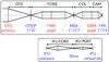 |
Fig. 1 Paraxial layout of the JWST telescope and NIRSpec optical train with elements at principal planes and the insert for the IFU case. Focal planes are blue; pupil planes are red. |
Summary of the parameters employed in the NIRSpec parametric model of the spectrograph.
The science instruments onboard JWST are located behind the Optical Telescope Element (OTE), which provides an image plane (OTEIP). As schematically shown in Fig. 1, the optical design of NIRSpec consists of three major blocks, all employing three-mirror anastigmats (TMAs) systems (te Plate et al. 2005). The light entering NIRSpec from the OTEIP is reimaged by the FORE optics onto the aperture plane of the MSA. The Filter Wheel Assembly (FWA), which carries the filters for spectral band selection (), sits in the pupil plane of the FORE optics. The collimator optics (COL) then projects the light from the slits onto the Grating Wheel Assembly (GWA), where another pupil plane is located. The GWA is equipped with various dispersers and a mirror for imaging (see ). Finally, the camera optics (CAM) focuses the (dispersed) beam onto the two detectors in the FPA.
The IFU entrance aperture is located in the MSA plane. For the majority of cases, IFU and MSA observations are mutually exclusive as their spectra share the same detector area and, therefore, all of the shutters have to be closed during IFU operations and the IFU entrance has to be blocked for multiobject exposures using the MSA. The IFU optics are split into an IFU FORE part, which reimages and rescales the MSA plane onto the slicer, and an IFU POST part, which picks up the 30 image parts and creates a virtual image for each slice at the MSA plane (virtual slits). The rest of the light path is then similar to the other observation modes.
The NIRSpec parametric model encapsulates all of the main optical elements identified in Fig. 1, but here we limit ourselves to the optimization of the parameters describing the spectrographic part of NIRSpec, that is the instrument from the MSA focal plane to the FPA. Although a parametric description of the PRISM is also part of the model, it was not optimized in this work and will be presented in a separate paper (see also Sect. 7).
There are two types of components in the NIRSpec parametric model: the parameterization of the coordinate transforms between the principal optical planes (here COL, IFU FORE, IFU POST, and CAM) and the geometrical description of the key plane elements (MSA, IFU slicer, GWA, and FPA). When we discuss coordinate transforms, we take the convention of naming so-called forward transforms those following the direction of the light path in NIRspec (i.e., from OTEIP to FPA). The type and number of the parameters specifying the various elements of the parametric model are summarized in . A more detailed description of each element is given below.
2.1. Optics
The TMAs in the NIRSpec optical train are manufactured to have only small amounts of distortion. It is therefore possible to model the individual optical transforms with a paraxial transform between the principal planes, and departures from the ideal paraxial system are treated as distortions and modeled using a fifth-order, two-dimensional (2D) polynomial. The IFU-FORE transform and the 30 IFU-POST transforms (one for each slice) also employ this formalism.
The paraxial part of a forward coordinate transform is defined by the magnification factors along the output axes γx and γy, the rotation angle of the coordinate system ϑ, and the position of the rotation center in the input and output reference frame (x0in, y0in) and (x0out, y0out). Given a point with coordinate (xin, yin) in the input plane, the equations in the Appendix A.1 provide the formulas to compute its corresponding coordinate (xout, yout) in the output plane, and vice versa.
2.2. Microshutter Assembly
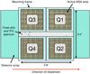 |
Fig. 2 Geometrical layout of the MSA projected onto the detector plane. The quadrants Q1–4 contain the microshutters; 5 high-contrast slits and IFU aperture positioned in the horizontal area in the center are indicated. |
The MSA is located at the slit plane of the instrument’s spectrographic part. This element, built at NASA GSFC, features four arrays of 365 × 171 microshutters, each 0.2′′ × 0.46′′ in size once projected onto the sky (respectively in the dispersion and cross-dispersion directions). The microshutters are arranged in a 2 × 2 mosaic, covering in total a FOV of 9 arcmin2 with ~250 000 individually addressable slitlets (Kutyrev et al. 2008). Mechanically, the microshutters have been implemented using micro electromechanical switches (MEMS), which each have an aperture size of 76 μm × 175 μm. The geometrical layout of the MSA module is shown in Fig. 2. As depicted in the figure, between the top and bottom quadrants, the five fixed slits are positioned together with the IFU aperture. Three of the high-contrast long slits have widths of 0.2′′, and one is 0.4′′ wide, and one is a square aperture of 1.6′′ × 1.6′′. The reference frame x-axis is aligned with the dispersion direction.
In the parametric model, the geometry of the MSA element is captured by a total of 40 parameters. For each of the four microshutter quadrants, we use the 2D coordinates of shutter (1,1) relative to the center of the FOV, a rotation angle, plus the shutter pitch size in x and y (for a total of 20 parameters). For each fixed slit, similarly, we have the center position and size in both dimensions. Each microshutter is labeled with an index for the quadrant and two indices denoting the column and row, (q,i,j), while the fixed-slits have names (S200A1, S200A2, S200B1, S400A1, and S1600A1). The MSA model parameters are used to transform from a shutter array index or slit ID with a simple geometrical calculation to its absolute physical position in the MSA plane (corresponding to the COL input plane), and vice versa.
2.3. Grating Wheel Assembly
The NIRSpec GWA is a cryogenic wheel mechanism that can be configured to position one of its optical elements into the beam path. It is equipped with six dispersion gratings (R ≈ 1000 and R ≈ 2700), a prism (R ≈ 100), and a mirror for the imaging mode (). The rotational degree of freedom of the wheel is given by a ball bearing controlled by two mechanisms: a cryogenic torque motor used as actuator and a spring operated ratchet to achieve accurate positioning. Despite the excellent mechanical performances of the grating wheel, the finite reproducibility of the positioning still causes small random displacements of the light beam on the focal plane each time the wheel comes back to a given position. To be able to predict the position of the light beam, two position sensors are used to accurately measure the tip and tilt displacement of each selected GWA element (Weidlich et al. 2008).
In the parametric model, the orientation of the GWA coordinate frame is such that the x-axis points in the dispersion direction, y in cross dispersion, and z in the beam direction. The diffraction of the six gratings is specified by their individual groove densities and front surface tilt angles. The double-pass PRISM dispersion is characterized by the front surface tilt, internal prism angle, and a relation with wavelength, temperature, and pressure dependence for the refractive index. The MIRROR is treated as a simple reflective surface.
The orientation of each disperser with respect to a reference surface at the GWA is given by four angles: one macroscopic front surface tilt angle between the grating surface and reference surface, Θy, plus three individual alignment angles (ϑx,ϑy,ϑz). The formalism that we employ to transform a light ray coordinate in the output plane of COL to the input plane of CAM passing through one of the elements of GWA are given by Eq. (A.1) to Eq. (A.9) in the Appendix A.2.
2.4. Focal Plane Assembly
NIRSpec’s FPA is equipped with two 5.3 μm cutoff, Teledyne HAWAII-2RG sensor chip assemblies (SCAs), provided by NASA GSFC (Rauscher et al. 2008, 2014). These HgCdTe sensors are ultra-low noise, state-of-the-art, near-IR detectors, which each have 2048 × 2048 pixels with 18 μm pitch size (corresponding to 100 mas on the sky); they are labeled SCA491 and SCA492, and aligned along the dispersion direction of the focal plane with SCA491 on the blue side (short wavelengths). The dispersion direction defines the x-axis of the FPA.
In the parametric model, the geometry of the FPA is captured by ten parameters: the absolute position 2D-coordinates, a rotation angle, and pixel-pitch in x and y for each array. These parameters are used to transform with a simple geometrical calculation from a pixel array index to its absolute physical position in the FPA plane (corresponding to the CAM output plane), and vice versa.
Information summary of the type of exposures acquired during NIRSpec testing, which were then used to extract the different type of reference data necessary for the model optimization.
2.5. Integral field unit
The NIRSpec IFU design is based around an image slicer element consisting of 30 stacked mirror surfaces that are curved and tilted with respect to each other so that the image is split into 30 individual slitlets, each of which is directed onto a dedicated pupil mirror (Closs et al. 2008). In this way, the 3′′ × 3′′ square FOV is dissected into 30 slices of 0.1′′ width (spectral direction) and 3′′ length (spatial direction). The spatial direction of the virtual slit is sampled at the FPA by 30 0.1′′-pixels, resulting in an IFU field consisting of 30 × 30 spaxels, each of size 0.1′′ × 0.1′′.
In the parametric model, the optical modules in the IFU are captured with the same combination of a paraxial transform with superimposed polynomial distortions as all of the other NIRSpec optics described above (Sect. 2.1). The IFU FORE optics consists of a transform between the MSA and slicer focal plane. The IFU POST part comprises 30 individual coordinate transforms, one for each slice, from the slicer to the virtual slit plane at the MSA. The IFU slicer itself is described by its absolute position and a rotation angle (in the IFU FORE output plane), whereas each slice is described by a relative position in the slicer and aperture size.
3. Calibration data
The data used for the model optimization process were acquired during the NIRSpec flight model performance verification and calibration campaign undertaken at the IABG testing facilities in Ottobrunn (Germany) in 2013. During two cycles of cryo-vacuum testing, NIRSpec was placed into a cryogenic chamber, under an inner shroud cooled by liquid helium to ~40 K, corresponding to NIRSpec operating temperature once in space. During testing, data were acquired from various light sources. We used both internal sources (housed in the CAA) and external lamps, housed within the cryogenic test setup and coupled to NIRSpec via the instrument pick-off mirror. All of the sources discussed here provide a spatially uniform illumination of the NIRSpec slit plane (Birkmann et al. 2012).
Three types of data are necessary for the optimization of the NIRSpec parametric model: imaging data, continuum spectra, and spectral lines. The first two sets provide spatial reference data, while the last set is used to derive spectral references. Illumination for imaging mode is provided by the CAA lamp labeled TEST; for continuum we used the CAA sources FLAT1, FLAT2, and FLAT3 that provide blackbody spectra for the three wavelength ranges 1.0–1.8 μm, 1.7–3.0 μm, and 2.9–5.0 μm, matched to the NIRSpec bands (). The spectral references are provided by the CAA source labeled REF, which is a rare earth absorption line source (erbium) with absorption features in the 1.4–1.6 μm wavelength range, and an external argon source, which emits unresolved lines in the range up to 2.5 μm. For these sources, the gratings of band II and band III were used in second and third order (as opposed to the default first order as in band I), while the FORE band-pass filters removed overlaps of the higher orders.
The data were acquired by cycling through exposures with the relevant light sources and different MSA configurations for each selection of disperser or for the mirror. To prevent overlapping among spectra when using any of the gratings, only one microshutter per MSA row was opened (Ferruit et al. 2012). The type of data collected for the model optimization are summarized in and described below in further detail.
3.1. Spatial references
For the imaging mode, we acquired exposures of the MSA, illuminated by the TEST lamp, in two different configurations: i) commanded fully open and ii) in a checkerboard pattern, a regular pattern of one open shutter for every three closed shutters, which can be seen in the enlargement in Fig. 3. In the full image, one can clearly notice the imprint of the shutters that fail to open, either because they are defective or because an entire row or column was masked to prevent electric shorts in the MSA arrays, in which case no shutter in that line can be commanded open.
When configured to fully open, the IFU aperture was also open, providing an image of the 30 virtual slits. The fixed slits are always open. As described in Sect. 5, these imaging exposures are used to first determine the approximate location of the MSA quadrants projected to the detector (fully open configuration) and then to derive the accurate FPA coordinates of the open shutters (checkerboard exposure).
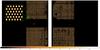 |
Fig. 3 Count-rate image of the two NIRSpec detector arrays (SCA491 and SCA492) of an exposure of the TEST lamp acquired in imaging mode (MIRROR) with the MSA configured in a checkerboard pattern, more clearly visible in the enlargement. SCA491 is on the left (blue side) and SCA492 on the right (red side). The images of the fixed slits are in the center of the images. Areas of defective shutters that fail to open are clearly visible and, in some cases, a full row or column is fully closed. The dark round feature in SCA492 is an area of dead pixels. This image was acquired with the old set of detectors and old MSA module. The image was generated from NIRSpec raw data following the steps described in Sect. 4. |
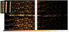 |
Fig. 4 Count-rate image of the two NIRSpec detector arrays (SCA491 and SCA492) of an exposure of the argon lamp acquired with G140M and the MSA configured in a dashed slit pattern (see enlargement). In this case the dashed slits were open in Q3 and Q4. The apparent width of the lines depends on the image scaling and blending of unresolved pairs. The regular pattern of spectra is spoiled by the missing spectra due to shutters that fail to open, or by misaligned, overlapping spectra from shutters that cannot be closed (stuck open). The image was generated from NIRSpec raw data using our preprocessing pipeline. |
To determine the FPA position of the spectra in the spatial direction, for each grating selection we acquired four exposures, with the MSA configured in four different patterns of multiple so-called dashed-slits and illuminated by the continuum flat-field lamp appropriate for that grating (i.e., FLAT1 for G140M and G140H, FLAT2 for G235M and G235H, or FLAT3 for G395M and G395H). A so-called dashed-slit consists of 14 shutters in a column, where an open shutter is followed by a closed one, yielding seven open shutters per slit. The four patterns were chosen to properly sample the MOS FOV, and are identical to those chosen for the acquisition of the spectral reference data. We placed ten dashed slits distributed in each quadrant, using alternatively Q1 and Q2, or Q3 and Q4. Figure 4 provides an image of spectra taken with one of the four MSA dashed-slit patterns.
3.2. Spectral references
Four exposures of the REF source were acquired for each grating for a first approximate measure of the location of the spectra on the FPA. For more accurate measurements of the FPA positions of a set of reference lines, we used four exposures of the argon source for each grating with the MSA configured in the four dashed-slit patterns described in Sect. 3.1. An example of these exposures for G140M can be seen in Fig. 4. In this image one can notice the missing spectra from the failed closed shutters, as well as misaligned overlapping spectra from defective shutters that cannot be commanded closed (stuck open).
The argon source was also used in combination with a fully closed MSA pattern and open IFU aperture and the grating G395H. To deal with the problem of failed open shutters interfering with the argon spectra from the IFU, we also acquired argon lamp exposures with a fully closed MSA and closed IFU aperture, providing an image of the contaminating signal of the failed shutters, which then can be subtracted away.
4. Data processing
All of the data presented here were acquired in full frame up-the-ramp mode, in which each detector pixel is sampled nondestructively every 10.74 s (see Rauscher et al. 2007 for more details on the instrument readout scheme). The two raw data cubes from all of the exposures were first processed to derive the count-rate images. This involves the following steps: bias subtraction, reference pixel subtraction, linearity correction, dark subtraction1, and up-the ramp fitting, as described in more detail in Birkmann (2011) and Böker et al. (2012). The output of these preprocessing steps are two FITS files (one for each detector) with image extensions for count-rate, variance, and quality flags for each pixel. Examples of count-rate images are shown in Figs. 3 and 4. If necessary, count-rate images of dedicated background exposures were subtracted from the calibration images to remove the spurious signal of failed open shutters.
When dealing with imaging exposures, preprocessing is all that is needed before analyzing the data. However, further computation steps are necessary for the spectral data. To extract spectra of the NIRSpec fixed-slits, MSA microshutters or the IFU from the count rate images, we developed the dedicated NIRSpec IPS Pipeline Software (NIPS), which uses the parametric model described in Sect. 2 to perform the following operations.
After having initialized the instrument parametric model to the appropriate observing mode, the location of the spectrum trace for a given slit, i.e., the curve of the slit center projected to the detector, is calculated between the lower and upper boundaries of the mode wavelength range using the model forward transforms for the slit coordinates in the MSA plane. The detector areas are then extracted as a subimage. Wavelength λ and spatial coordinates dy are assigned to each pixel in the subimages according to the combination of slit, filter, and grating by a computational method that we call “meeting at the grating”, described in Appendix A.3. The result of this operation is a 2D spectrum, irregularly sampled in λ and dy. From this data, it is already possible to calculate irregularly sampled spectra with extraction operations working in the pixel columns or pixels belonging to wavelength bins.
The next step is the generation of a so-called 2D-rectified spectrum, for which the data in the subimage is resampled onto a regular grid of wavelength and spatial coordinates. Finally, the one-dimensional (1D) rectified spectrum is computed as the median along the spatial direction in each wavelength bin of the 2D-rectified spectrum using only pixels with the selected quality flags. For all of the data sets, dead (i.e., unresponsive) pixels were flagged and not used in the computation of the 1D spectra. The spectra were all derived at the NIPS default resolution for each disperser, given by the Nyquist sampling of the nominal resolution of the disperser at the central wavelength ().
The NIPS only utilizes a single thread per execution, which means that the extraction and rectification of hundreds of spectra for each grating was a lengthy process; in fact, in terms of computation time this was the lengthiest step of the model calibration. On average, the extraction and rectification of 100 MOS spectra from a high resolution grating took about 30 minutes on a state-of-the-art workstation CPU.
4.1. Reference data
After these general processing steps, the reference data used by the model optimization procedure were generated. For the imaging mode, we measured the centroids of the slit images. The input was an exposure with the 3 × 3 checkerboard pattern (similar to Fig. 3) during which the fixed slits and IFU virtual slits were also illuminated. At first, the location of each open shutter on the detector was predicted with our initial guess for the parametric model. The shutter images typically cover 2 × 5 pixels, and their surrounding area was cut and examined for bad pixels. If this subimage contained invalid pixels it was discarded, along with those of known failed closed shutters or those with insufficient signal (because the corresponding microshutter had unpredictably failed to fully open). Finally, the geometrical centroid of the area around the predicted slit image was calculated, while taking care not to include pixels illuminated by the adjacent open shutters. The subimages of fixed slits and IFU virtual slits were processed in a similar way, but were not filtered for defective pixels since the slit images are much larger in the spatial direction and, therefore, their centroids are less influenced by bad pixels.
The reference data from spectra were created with the NIPS using an intermediate model in the course of iteratively adjusting the parameters. The final measurement output for a slit consisted of pixel coordinates (iref,jref) as a function of the true wavelength λref. To obtain accurate reference points despite a model with, at this point, still insufficient accuracy, the following approach was taken. For the references in the spatial direction, the location of the continuum spectra for the opened shutters were predicted with the available model and subimages were cut from the data. To measure the spectral trace position, the centroid in each pixel column was calculated in a range slightly larger than the spectrum width. The results were restricted to areas without contamination by neighboring or failed open shutters. For each spectrum, the centroid along the columns was then fitted with a fourth-order polynomial j = Pj(i) with 4σ rejection of outliers, in particular to eliminate the small-scale influence of bad pixels.
For the references in the spectral direction, the argon line spectra were rectified and collapsed to 1D using the median value across the slit. For each grating, a set of 12–35 isolated lines was selected from the spectrum and the profiles were individually fitted with a Gaussian in the range of ± 5 spectral pixels around the predicted line location. For a given line, this fit provided the wavelength assigned by the model λm. The model-predicted detector pixel position of the line (im,jm) was then calculated with the coordinate transforms from the slit to the detector for λm. However, the true detector position (iref,jref) is different, since the intermediate model was not perfectly accurate. In the spatial direction, the model trace generally does not match the measured trace Pj(i). As a result of the line profile fit and model calculation, im is the coordinate of the intersection between the model trace and line image. Because of the slit tilt and the trace offset, im is therefore different from iref. Typical values for the trace position difference of the gratings were about 0.5 px (see below in ), and the slit tilt is <8° for the R2700 and <4° for the R1000 gratings. Therefore, the difference in the spectral direction coordinates was generally <1/14–1/29 of a pixel, which is far below the 0.2 px RMS allocation in the spectral calibration budget, and was neglected by setting iref = im. The reference position in the spatial direction was then computed from the trace polynomial as jref = Pj(im). Combining the pixel coordinates and the true wavelength of the emission line, the reference tuple (iref,jref)(slitID,λref) was obtained for each slit and line and could then be compared to the model calculated positions for the true wavelength  .
.
5. Model optimization procedure
Because NIPS uses the transforms of the parametric model to obtain the reference data, the optimization of the model had to follow an iterative approach. The spectra from the different reference data sets listed in were extracted from the count-rate images with an increasing level of accuracy in terms of wavelength and spatial location within the slit, while we progressed through the various steps of our model optimization process. At first, NIPS operated with our initial best-guess of the NIRSpec parametric model and the output data are characterized by only approximate wavelength and spatial coordinates. The model parameters were then adjusted, manually at first, and then via a proper optimization procedure, so that the final results reach a high level of accuracy.
The initial parameters of the instrument model were obtained from subsystem tests or optical modeling. The manufacturer Reosc (Sagem) delivered a parametric description of the TMA modules to Airbus DS, who then assembled a complete as-built optical model of NIRSpec in the commercial optical design software Zemax2. We traced grids of rays through this prescription and derived the parameters of the paraxial and distortion transforms from the calculated ray coordinates. The IFU transforms were obtained in a similar way, but here we relied on the as-designed Zemax model of this subsystem.
The information about the fixed slits and MSA quadrant positions and pitches are from subsystem measurements at warm transformed to cold conditions and were supplied by NASA GSFC. The grating dispersion and front surface tilts were set to the ambient design values provided by the manufacturer. We had no information about the relative alignment angles of the GWA elements, so they were set to 0 in the beginning. As a starting point for the FPA, we assumed perfectly aligned detectors without rotation in accordance with the nominal values provided by NASA GSFC.
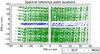 |
Fig. 5 Location of spectral reference points in the global model optimization. These reference points consist of the positions of argon emission lines taken with the gratings G140M, G235M, G395M, and G395H. In total, there are 28 020 points distributed over both detectors. The top and bottom groups of green dots are from shutter spectra; the central blue crosses from the fixed slits. |
5.1. Model assumptions
Residuals of the forward projection from MSA to FPA before and after the global model optimization from gratings and the MIRROR on the detector.
The instrument description partly offers more flexibility than needed, since some parameters are degenerate. For instance the distortion polynomials have low-order terms that mimic a magnification or constant offset, which are also present in the paraxial description. Then again, such offsets can be captured by the parameters of the focal plane elements. To avoid degeneracies, set absolute references, and avoid unnecessary complexity, the final model was created with the following premises:
-
The GWA MIRROR has all alignment tilt angles at 0 and definesthe GWA reference plane. All other dispersers have alignment tiltangles relative to this surface.
-
The MSA quadrants are rectangular and regular in size, i.e., in an individual quadrant the shutter pitch is uniform and the shutter axes are perpendicular.
-
The FPA gap is forced to be centered on the y-axis. SCA 491 has no rotation and is symmetrical to the x-axis. SCA 492 is free to move and rotate within the first condition that couples the positions of 491 and 492. This does not restrict the modeling of the instrument, as the movements can be compensated by the distortion polynomials of the CAM. It does, however, produce a geometrically simple FPA description without excessive tilts and offsets.
-
The COL and CAM transform are assumed to be achromatic (all-reflective optical parts) with no wavelength dependence of the distortion coefficients.
5.2. Manual adjustment
As mentioned before, the model fit was carried out based on data extracted with an unoptimized initial model, hence the pixel coordinates of the spectra were not accurately known. To avoid the contamination of reference data by nearby slits and shutters during the extraction, it was necessary to locate the spectra with an initial accuracy better than 1 pixel, in particular in the spatial direction. Therefore, the first steps in the calibration were a manual adjustment of the detector, fixed slit, and MSA quadrant positions and pitches. Imaging data of the slits and the fully open MSA were plotted with the projected slit and MSA shutter outlines. Known failed closed shutters created a quasi-random pattern, in particular at the quadrant edges, and allowed us to match the exposure with the model prediction. From the offsets, the change of the positional parameters was visually deduced and fed into the model. The same approach was taken to narrow down the positions and rotations of the IFU virtual slits, although only after having optimized the spectrograph optics. In addition, spectra of the fixed slits with the Erbium absorption source were used to estimate an offset in the spectral and spatial direction. In this case, the alignment angles of the dispersers were adjusted to achieve a visual match between the predicted and measured positions of the traces and known absorption features. The intermediate model was then accurate enough to enable the derivation of the reference data as previously described in Sect. 4.
All of the necessary processing and visualization scripts for the manual adjustment had been prepared and tested with simulated data beforehand. Therefore, this step could be carried out very efficiently once the real data were available and it was completed within a day.
5.3. Automated optimization
The calibration of the parametric model was eventually carried out with an automated optimization in multiple steps. The common principle was to minimize the residuals between model predicted and true coordinates from the reference data with least-squares fits, during which selected subsets of the parameters were modified.
The first step of the optimization covered the forward transform from MSA to the detector. In this step, we treated the global characteristics of the spectrograph, hence 120 parameters were fitted simultaneously, consisting of MSA quadrant positions, pitches and rotation, COL forward distortion, GWA disperser tilt angles, CAM forward distortion, and FPA positions and rotation (compare with ). The fixed slit positions in the MSA were not optimized at this stage because their images in combination with the predefined MIRROR orientation served as an absolute reference for the detectors. To obtain a reliable and spatially unbiased description of the optical distortion, the reference data set was constructed from a selection of the GWA elements whose points cover the FPA plane as evenly and wide as possible. The gratings G140H and G235H have an asymmetric distribution of lines on the detectors concentrated on SCA 492, and these were left out in the beginning to prevent an imbalance in favor of this side of the field. Therefore only the data of the gratings G140M, G235M, G395M, and G395H were used, which each have 4000–10 000 reference points that extended almost fully up to the FPA edges and evenly cover the two SCAs. Combining the data of the fixed slits and four different MSA configurations per grating led to a total number of 28 020 spectral reference points as shown in Fig. 5. The MSA imaging reference data contained 23 727 centroids in total. To obtain a similar amount of points as for the other GWA elements, about 1500 of them were randomly selected per quadrant, yielding 5982 reference centroids, including the fixed slits. Therefore, in total 34 002 points were available for the global model optimization. We defined a function comparing the pixel positions calculated by the model with the reference data, and we minimized the residuals by optimizing the model parameters with a least-squares fit. To reject outliers, the points were filtered with a 4σ clipping in each subset of the same slit type (fixed slit or MOS), pixel coordinate direction, GWA element, and detector in each residual calculation. Despite the large amount of reference points and free parameters, the least-squares minimization process was not particularly computationally expensive and was run on a normal workstation, taking approximately 1 h (using only one thread).
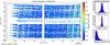 |
Fig. 6 Residuals of forward coordinate transforms from MSA to FPA for all of the gratings on the detectors. Left panel: distribution in the detector focal plane. The spectra of the shutters are the wide bands on top and bottom; the stripes in the center are from the fixed slits. Right panel: histograms of residuals in pixels in i and j direction (top, middle) and absolute residuals (bottom). Shown in red are the confidence limits of 68.27% around the median at −0.060 and + 0.062 (i), and at −0.025 and + 0.028 (j), and the limit of 68.27% of absolute residuals (0.071). |
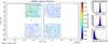 |
Fig. 7 Residuals of forward coordinate transforms from MSA to FPA for the imaging mode on the detectors. Left panel: distribution in the detector focal plane. The four quadrants of the MSA are clearly visible, the five fixed slits are visible in the center area. Isolated shutters and slits are disturbed by bad pixels, in particular Q3 (top left). Right panel: histograms of residuals in pixels in i and j direction (top, middle) and absolute residuals (bottom). Shown in red are the confidence limits of 68.27% around the median at −0.023 and + 0.022 (i), and at −0.038 and + 0.034 (j), and the limit of 68.27% of absolute residuals (0.046). |
In a second step, the positions of the fixed slits were optimized individually because their initial positions may not be optimal in combination with the new COL distortion, which was dominated by the MOS data in the previous optimization (≈20 × more shutter references than for fixed slits). Therefore, another fitting run was performed, only changing the SLIT positions in the MSA, using their reference data. In a third step, we adjusted the alignment tilts of the two remaining gratings G140H and G235H to complete the forward transforms, taking the same minimization approach with their so far unused reference data.
The initial and final residuals on the FPA for fixed slits and MOS are listed in , the final ones are also shown in Fig. 6 for the gratings and Fig. 7 for the imaging mode. As expected, the optimization brought the residuals on the detectors to an average of zero, while reducing the standard deviations of the gratings by a factor of about 13–21 from 0.43–1.6 to 0.033–0.076 px. Some residuals are still on the order of 0.4 px, however, these correspond to single argon lines, where the Gaussian fit was disturbed by nearby faint lines that were not detected in the line selection. 68.27% of the values of the absolute residual (geometrical norm of both axes) are below 0.071 px (a limit similar to 1σ in a Gaussian distribution). In imaging mode, the optimization was equally successful, reducing the residuals to an average of zero and their RMS by 6–16× to about 0.04 px. Calculating the absolute residuals, 68.27% of the values are lower than 0.046 px, which confirms the model accuracy. Nevertheless, some of the shutter centroids are disturbed by bad pixels, especially in Q3 (lop left). The large offset of the S200A1 (one of the left fixed slits) is likely caused by a low-QE pixel in the slit image and thus inaccurate centroid data. The robustness of the optimization was confirmed by rerunning the procedure with different initial parameters, where we obtained the same final model.
The parametric model is not only used to project from the slits to detector, but also backward from FPA to the slit plane. In fact, this direction is essential for the spectrum extraction and calculations for the target acquisition. Therefore, two more steps were also necessary to optimize the backward transforms of the optical elements. The CAM backward distortion was adjusted with the same reference data set as in the global fit, selecting the points G140M, G235M, G395M, G395H, and the MIRROR. This optimization worked at the GWA exit plane in angular coordinates, since this is a pupil plane. The MSA positions of the slits were transformed forward through the optimized COL and GWA. The residuals were calculated as the difference between those projected slit position, and the positions of the detector reference points, transformed backward with the CAM model. As in the previous steps, the backward distortion parameters of the CAM were optimized with a least-squares fit and 4σ clipping. This approach was chosen to make the CAM backward transform optimal with respect to the COL forward transform, which is the same combination used during the wavelength calculation in the spectrum extraction (see Appendix A.3).
In the second step, the COL backward distortion was optimized with the identical reference data set. To obtain a consistent transform from FPA to MSA, the reference points on the detector were propagated backward through the now optimized CAM and GWA elements to the GWA input plane. The residuals were calculated between the detector references transformed further backward through the COL and the slit positions in the MSA plane. The distortion parameters were again optimized with a least-squares fit and 4σ clipping. With this step completed, the model was tuned to mimic the spectrographic part of the instrument for SLIT and MOS mode with all of the gratings and the MIRROR in both directions.
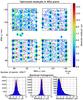 |
Fig. 8 Combined residuals of the backward transform from FPA to MSA for G140M, G235M, G395M, G395H, and the MIRROR. Top panel: distribution in the MSA plane. The residuals of shutters used in the spectral modes (groups of the dashed slits) vary more strongly than those of the shutters from imaging mode (points spread in the quadrants). The physical direction of the axes are inverted to match the images of the detectors, since the reference frames are not following the optical projection. Bottom panel: histogram of residuals in x and y direction (left, middle) and absolute residuals (right). Shown in red are the confidence limits of 68.27% around the median at −1.84 and 1.98μm (x), and at −1.07 and 1.12μm (y), and the limit of 68.27% of absolute residuals at 2.44μm. |
The residuals of the complete backward transform from the detectors to the MSA plane are shown in Fig. 8 for the GWA elements used in the optimization (G140M, G235M, G395M, G395H, and the MIRROR). The combined residuals are close to 0 μm on average with a standard deviation and 68.27% limit of absolute residuals around 2 μm, which is equivalent to 1/38 of a shutter aperture width. The imaging residuals alone are slightly more accurate with variations of around 1.4 μm that are 1/54 of a shutter aperture width. This is also apparent in the image, where the shutters of the spectral modes (groups of the dashed slits) show some larger residuals than those of the imaging mode (shutters spread in the quadrants). However, the large residuals originate from problematic lines already seen in the forward direction (Fig. 6) and are not representative of the average accuracy, as can be seen in the histograms.
The last subsystem missing in the spectrograph, the IFU, was handled independently, since its model offers the flexibility to adapt itself to the previously obtained parameters of the other components. In the COL, the IFU virtual slits inject the light slightly outside the MSA field, but their position can be freely adjusted in the model, and in the CAM, the light mostly travels on paths common with the spectra of other modes. At first, the virtual slits in the MSA plane were manually moved so that their projected outlines match their images on the detector and obtain an accuracy <1 px for the reference data creation. Following this, 30 centroids of the virtual slit images and 918 spectral reference points were extracted in the same way as for the other slits, using exposures with the MIRROR and G395H grating and the argon and continuum lamps. As in the global forward optimization, the virtual slit positions were fitted by minimizing the residuals between the model predicted and measured positions on the detector.
Since the default reference data is averaged across the spatial direction, it does not contain any information about the slit rotation. The IFU slice spectra are rather wide (30 pixels) and on this scale the optical distortion influences the tilt of the slit projection. Therefore we performed another fitting round to adjust the rotation of the virtual slits. Besides the references for the center, we extracted reference points from only the top and bottom half of the slice spectra, corresponding to traces at positions of ± 0.25 in the relative aperture and yielding additional information for the top and bottom half. In this way, we obtained three reference points for each emission line at the relative positions−0.25, 0, and + 0,25 inside the slice, which allowed us to verify the slit rotation. To determine the spectral coordinates, the argon spectra were averaged only across the semislices, and the line positions λm were measured with a Gaussian fit as before. However, in the spatial direction it is not possible to derive the centroids of only half a spectrum, so no polynomial function Pj(i) could be constructed to calculate the pixel coordinates. Nevertheless, after the preceding optimization, the model was already accurate in the spatial direction (the residuals were <0.1 px), therefore the spatial trace was calculated with the instrument model at the offset slice position. Finally, in total we obtained 2778 points for the optimization, including the imaging centroids.
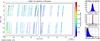 |
Fig. 9 Residuals of transforms from IFU slices to FPA with G395H. Left panel: distribution in the detector focal plane. The errors increase toward the lower left, where the CAM distortion was not influenced in the global fit and is not optimal for the IFU, but remain <0.25 px. Right panel: histograms of residuals in pixels in i and j direction (top, middle) and absolute residuals (bottom). Shown in red are the confidence limits of 68.27% around the median at −0.054 and + 0.058 (i), and at −0.004 and + 0.009 (j), and the limit of 68.27% of absolute residuals (0.068). |
The final residuals of the forward transform with the IFU and the grating G395H are shown in Fig. 9. The 68.27% limit of absolute residuals is 0.068 px and similar to the SLIT and MOS modes; the errors increase only toward the left edge. This is an area not covered by the MOS and SLIT data during the CAM distortion fit, therefore the optics model is not as accurate in that area. Nevertheless the residuals there are sufficiently small with <0.2 px. The spatial direction j is almost perfectly met, while the spectral direction and absolute residuals show a distribution similar to the other gratings in the global optimization step. The IFU imaging residuals (not displayed) in the upper half of the left SCA 491 are disturbed by bad pixels and not reliable, similar to the MOS mode. The true accuracy of the centroids is likely better than the calculated 68.27% absolute residual limit of 0.14 px.
6. Results
To verify the self-consistency of the optimized model, we examined the resulting parameters for unrealistic values, which could mean that these values are degenerate with others or were not properly constrained during the fit sequence. However, no unusual numbers were found in the results.
Optimized geometrical parameters of the MSA model.
The MSA quadrants have pitches that differ by only 0.02 μm in the spectral and 0.15 μm in the spatial direction amongst them (see ). The individual rotation angles are below 0.03° absolute. The variations of fractions of microns and few arcminutes indicate the high consistency of the model. The FPA was forced to end up in a symmetric model (as mentioned in Sect. 5.1). The fitted gap is 2.61 mm, and is very close to the nominal value of 2.75 mm, the rotation of SCA 492 is very low with 21.5 arcsec.
Optimized alignment tilt parameters of the gratings relative to the MIRROR surface.
The alignment angles of the gratings relative to the MIRROR surface are listed in . They generally show a large tilt of about 17′ around the z-axis (perpendicular to the surface), which may be caused by freezing the CAM and FPA rotation, so that any other rotation in the field was transferred to the GWA parameters. The tilt around the other axes x (cross-dispersion movement) and y (dispersion movement) are in the range of ±100′′ and are consistent relative to each other. Only G395M has a larger tilt of about 200′′ around x, which is evident in the exposures, where the spectra are located significantly lower on the detector compared to the other gratings.
The optical distortions of COL and CAM are largely dominated by low-order effects. When re-deriving the paraxial magnifications and rotations from the new coordinate transforms, they would only change by <0.4% and <0.015° compared to the as-built model. Therefore, the optimized transforms are very close to the initial transforms from the Zemax prescription, giving us confidence in the fitted model as well as the as-built optical prescription.
6.1. Spatial accuracy
Residuals of calculated trace positions in the spatial direction compared to the measurements extracted with the optimized model.
Residuals of extracted argon emission lines comparing the measured line wavelength with the true wavelength.
One specific way of testing the model is the verification of the spectrum trace positions. To do this, using the optimized model, trace measurements were again extracted from the calibration data in the same way as described in Sect. 4. The centroids in each pixel column of continuum spectra were fitted with a fourth-order polynomial with 4σ clipping. The calculation was carried out for all of the gratings for SLIT and MOS. For the IFU, only the data of G395H had clean traces and were analyzed in the same way. The exposures of other gratings that had not been used for the optimization were also processed, and clean areas of the spectra (no failed open shutter spectra) were selected manually. Then, the slit centers were projected to the detector with the parametric model in the respective spectral range and the difference to the polynomials was computed for each column. The average residuals in the spatial direction are listed in , along with the standard deviation. The mean differences are typically <0.05 px and close to zero. The scatter is <0.1 px and even smaller for the medium resolution gratings. The IFU is similarly accurate in all of the gratings, although it has only been fitted with the G395H grating.
In imaging mode, the ability to reproduce the location of the slit images on the detector was already verified during the model optimization. The large number of about 6000 randomly selected and manually inspected shutters used on input ensured a proper sampling of the FOV of NIRSpec. This gives us confidence that the residuals shown in Fig. 7 and listed in are representative of all of the positions within the FOV. Their standard deviations of 0.025–0.044 px represent an accuracy that is sufficient to meet the overall NIRSpec target acquisition error budget.
6.2. Spectral accuracy
The second important test of the parametric model is the extraction of spectra and verification of the spectral accuracy. Therefore, the argon lines from the input exposures were extracted to 1D spectra with the optimized model, the lines fitted with Gaussian functions, and their measured wavelengths compared to the true values. The range below 1 μm was also examined for the band I gratings, which had not been covered by continuum spectra and thus was missing in the fit reference data. In the IFU case, all of the slices for all of the dispersers were processed, as the impact of failed open shutters on the output was found to be negligible. Lines that were known to be problematic during the model optimization were not taken into account.
The residuals of the modes and dispersers are listed in ; they are individually clipped at 4σ. All of the gratings are accurately calibrated with a residual scatter around 0.08 px for the R2700, and 0.05 px for the R1000 dispersers, corresponding to 1/25 and 1/40 of a resolution element of 2 px, respectively. As an example, the G140H MOS data are shown in Fig. 10. The plot contains the residuals in pixels of each line from each spectrum with the error assigned during the Gaussian fit. The majority of the points lie within ±0.2 px and have negligibly small errors, and the overall standard deviation is 0.083 px. The lines at wavelengths below 1 μm are also well calibrated, although the model has not been optimized with data in this spectral range. Somewhat larger errors appear toward the longer end of the wavelength range, but can be attributed to random measurement errors.
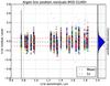 |
Fig. 10 Extraction residuals of the argon lines in the MOS data taken with filter F140X and grating G140H, given in detector pixels. In the main panel, each measured line position from each spectrum is plotted with the error from the fit. The mean residual is −0.019 px with a standard distribution of 0.083 px. The points outside the 4σ-limit of the data are excluded as measurement errors. The right panel shows the distribution of the combined residuals of all lines. |
7. Discussion and conclusion
The results presented here show that the method we developed yields an intrinsic spatial accuracy of the parametric model that is better than 1/10 of a pixel. The model wavelength calibration is equally accurate, showing RMS residuals equivalent to approximately 1/20 of a resolution element or, in other words, at the level of 5–7 km s-1 for all of the gratings and any of the NIRSpec modes (fixed slits, MOS, and IFU). This is two times better than the formal standard deviation allocation of 0.2 pixel (or 1/10 of a resolution element) specified for this step in the overall wavelength calibration budget of NIRSpec.
Reaching an even higher model precision would require more accurate reference data. The Gaussian fit of some emission lines is problematic when their measured wavelength is influenced by blending from nearby faint lines. In Fig. 10 this appears as a bulk shift of the residual cloud of a few lines, for example, in the line pair at 1.35 μm. Here the method reaches the limit of inspecting individual lines and a fit of a line catalog could help to increase the model accuracy further.
One limitation of this study is that the assessment of the wavelength calibration accuracy is carried out, for the most part, on the same data points from the same apertures that were used to optimize the parametric model. During the limited time of the calibration campaign, we did not acquire suitable additional data that would allow us to assess, in a direct and clean manner, the wavelength calibration accuracy from spectral lines from an independent set of MOS apertures.
We note, however, that the optimization results in terms of the distortions of the COL and CAM optics are extremely regular and smooth, as can be seen from Fig. B.1. This indicates that the optimization process is not driven by the residuals of some individual lines/apertures, but a global solution is obtained that reflects the macroscopic properties of the optical system. Therefore we expect that comparable levels of accuracy can be achieved for all of the MOS apertures on a different set of unresolved spectral lines. Indeed, as mentioned in Sect. 6, this is supported by the accuracy of the wavelength calibration of the argon lines in the range lower than 1 μm that (in the camera) sample different light paths from any of the reference data.
So far we have not addressed the model accuracy for the large square-shaped S1600A1 slit (intended for exoplanet transit observations). This is because it was not practicable to fit argon lines to the large slit function, so the only reference data available for this aperture are the slit image centroid coordinates. However, the centroid measurement is very robust thanks to the image extension of 16 × 16 px2, and in combination with the other elements of the parametric model, and in particular the smoothness of the coordinate transforms, it is expected to lead to an extraction of its spectral data with an accuracy comparable to that of the other slits.
For a similar reason, we have not presented the results of the wavelength calibration for the prism. The emission lines of the argon source cannot be used as wavelength reference in this case, because they are heavily blended at the prism resolution of ~100. Thus, a different data set is necessary for the calibration of the prism. We plan to make use of data from three of the instrument calibration sources of the CAA. These three sources employ Fabry-Perot type interferometric filters that provide six well-defined transmission features over band I, II, and III. The accurate center of gravity of these features at NIRSpec operating temperature can be determined from the spectra obtained with high resolution gratings, in a way bootstrapping the wavelength calibration for the prism via that of the gratings presented here. The results of this approach will be shown in a forthcoming paper.
The accuracy of the model transformations for the spectrographic part of the instrument is a crucial part in the overall process of the NIRSpec wavelength calibration, but it is not the only part. There are two other important contributors to the overall wavelength calibration budget: the calibration of the spectrum shift caused by the finite repositioning accuracy of the grating wheel (see Sect. 6.1) and the mixing of spatial and spectral information when our apertures are significantly larger than the size of the point-spread function (so-called slit effect). Concerning the grating wheel-induced shift, preliminary results from De Marchi et al. (2011) have shown that there is a tight linear relation between the telemetry readings of the GWA sensors and the tilt of a disperser element. These calibration relations are implemented during the spectral extraction to correct for the actual disperser orientation. Current analysis using ground test data shows that this correction leads to an additional contribution to the uncertainty of the wavelength calibration of approximately 1/16 of a pixel, which is a fraction of the model uncertainties.
The calibration data presented here were acquired in 2013. In the meantime, the MSA and FPA subsystems of the instruments have been replaced. The quadrants of the new MSA have a smaller number of stuck closed shutters (less than 10%) and the new FPA unit features two new H2RG detectors, which are not affected by the performance degradation problem of the older model (Rauscher et al. 2014). Therefore, the instrument model needs to be updated to reflect the changes in the optical geometry of these elements, which, however, are expected to be small. For this purpose, we acquired a new set of imaging and spectral reference data to be used for a new iteration of the model optimization during the most recent cycle of cryogenic tests that the instrument underwent in the Space Simulator Facility of NASA GSFC at the end of 2015 and beginning of 2016. These tests involved all four scientific instruments onboard JWST in their flight configuration and integrated in the JWST Integrated Scientific Instrument Module (ISIM).
Planned updates of the NIRSpec parametric model following major milestones of the JWST project.
As the assembly of the space telescope proceeds, various environmental tests are planned for the different levels of the system integration. As summarized in , tied in with this overall schedule is our plan for three updates of the NIRSpec instrument model and further assessment of the wavelength calibration accuracy. The first model update will take place once the set of recently acquired data have been reduced. In this case, an analysis of the spectral reference points from different MSA apertures and for a large set of GWA repositioning will be carried out to assess the comprehensive accuracy of the spectrograph wavelength calibration, over light paths not used for the model optimization itself and including the uncertainties of the GWA sensor calibration.
A new update of the model using the data acquired during the cryo-vacuum campaign at OTE-ISIM level will follow. This will allow us to assess the impact of the mechanical and thermal stresses that the instrument will undergo during the preceding series of vibration and acoustics tests (see ) on its overall alignment, and therefore, possibly, on the model parameters. The third and (likely) last update of the parametric model will take place soon after launch. We expect the mechanical and thermal environment of the telescope in space to be very stable and, therefore, once in operation, new model updates should not be necessary, although regular monitoring of the instrument wavelength solution will be performed.
Nevertheless, the model calibration presented here remains the keystone of all future model recalibrations. This is because, unlike during the 2013 test campaign, in the NASA testing facilities and in space we do not have access to an argon source that provides us with a set of independently and well-calibrated spectral references. The upcoming model updates will be carried out using NIRSpec internal calibration sources housed in the CAA. The wavelength of the emission and absorption features of these sources, however, was not known (from the manufacturer measurements and subsystem level tests) with the tenth-of-a-nanometer level of accuracy that we require for the NIRSpec wavelength calibration. To address this, during the 2013 test campaign, together with the argon exposures we also acquired exposures of the internal sources and we used the model calibration presented here to obtain the wavelength calibration of the spectral features of the internal sources to the required accuracy.
Finally, for the sky observations and the target acquisition, the calibration of the optical paths through the FORE elements of NIRSpec has to be combined with the calibration of the telescope optics and will be also carried out during the commissioning period, once the instrument is in space. Using the data acquired from observations of an astrometric field in imaging mode, the parameters of the FORE transform for each filter element in combination with that for the OTE will be determined. This step will complete the spatial and spectral calibration of NIRSpec prior to the start of any scientific activity.
In summary, the work presented here discusses the first and crucial aspect of the NIRSpec wavelength calibration strategy: the optimization of the instrument parametric model. We have developed a procedure that uses the calibration data acquired for a limited subset of the NIRSpec modes, and in particular only 1.5% of the quarter of a million NIRSpec slits, to derive a highly realistic model of the instruments optical geometry. This model allows us to compute accurate light paths within the instrument and hence predict the spatial and wavelength positioning of the spectra for all of the instrument apertures and modes with an accuracy exceeding the formal requirement by a factor of two.
Dark subtraction is carried out at the data cube level, i.e., the corresponding frame from a low-noise dark-currents cube is subtracted from each frame of the exposure.
Acknowledgments
This work was funded in part by the Marie Curie Initial Training Network ELIXIR of the European Commission under contract PITN-GA-2008-214227.
References
- Bagnasco, G., Kolm, M., Ferruit, P., et al. 2007, in SPIE Conf. Ser., 6692 [Google Scholar]
- Beletic, J. W., Blank, R., Gulbransen, D., et al. 2008, in SPIE Conf. Ser., 7021 [Google Scholar]
- Birkmann, S. M. 2011, Description of the NIRSpec pre-processing pipeline, Tech. Rep. NTN-2011-004, ESA/ESTEC [Google Scholar]
- Birkmann, S. M., Ferruit, P., Böker, T., et al. 2012, in SPIE Conf. Ser., 8442 [Google Scholar]
- Böker, T., Birkmann, S., de Marchi, G., et al. 2012, in SPIE Conf. Ser., 8442, 84423 [Google Scholar]
- Closs, M. F., Ferruit, P., Lobb, D. R., et al. 2008, in SPIE Conf. Ser., 7010 [Google Scholar]
- De Marchi, G., Te Plate, M. B. J., Birkmann, S. M., et al. 2011, in SPIE Conf. Ser., 8150 [Google Scholar]
- Ferruit, P., Bagnasco, G., Barho, R., et al. 2012, in SPIE Conf. Ser., 8442 [Google Scholar]
- Gardner, J. P., Mather, J. C., Clampin, M., et al. 2006, Space Sci. Rev., 123, 485 [NASA ADS] [CrossRef] [Google Scholar]
- Gnata, X. 2007, Ph.D. Thesis, Université Claude Bernard Lyon 1, France [Google Scholar]
- Kutyrev, A. S., Collins, N., Chambers, J., Moseley, S. H., & Rapchun, D. 2008, in SPIE Conf. Ser., 7010 [Google Scholar]
- Piquéras, L., Legay, P., Legros, E., et al. 2008, in SPIE Conf. Ser., 7017 [Google Scholar]
- Piquéras, L., Legros, E., Pons, A., et al. 2010, in SPIE Conf. Ser., 7738 [Google Scholar]
- Rauscher, B. J., Fox, O., Ferruit, P., et al. 2007, PASP, 119, 768 [NASA ADS] [CrossRef] [Google Scholar]
- Rauscher, B. J., Alexander, D., Brambora, C. K., et al. 2008, in SPIE Conf. Ser., 7021 [Google Scholar]
- Rauscher, B. J., Boehm, N., Cagiano, S., et al. 2014, PASP, 126, 739 [NASA ADS] [Google Scholar]
- te Plate, M., Holota, W., Posselt, W., et al. 2005, in SPIE Conf. Ser., 5904, 185 [Google Scholar]
- Weidlich, K., Fischer, M., Ellenrieder, M. M., et al. 2008, in SPIE Conf. Ser., 7018, 21 [Google Scholar]
Appendix A: Coordinate transforms formalism
Appendix A.1: Transform between optical planes
The coordinate transforms in the NIRSpec model use a paraxial transform between the principal planes. Departures from the ideal paraxial system are treated as distortions and modeled using a 2D polynomial.
The paraxial part of a forward coordinate transform is defined by the magnification factors along the output axes γx and γy, the rotation angle of the coordinate system ϑ, and the position of the rotation center in the input and output reference frame (x0in, y0in) and (x0out, y0out). From the input coordinates (xin,yin), the paraxial output coordinates (xp,yp) are given by ![Mathematical equation: \appendix \setcounter{section}{1} \begin{eqnarray*} x_{\rm p} &\!\!\! =\!\!\! & \gamma_x \cdot \left[(x_\mathrm{in} - x_{0\,\mathrm{in}})\cos(\vartheta) + (y_\mathrm{in} - y_{0\,\mathrm{in}})\sin(\vartheta)\right] + x_{0\,\mathrm{out}} ,\\ y_{\rm p} & \!\!\!=\!\!\! & \gamma_y \cdot \left[-(x_\mathrm{in} - x_{0\,\mathrm{in}})\sin(\vartheta) + (y_\mathrm{in} - y_{0\,\mathrm{in}})\cos(\vartheta)\right] + y_{0\,\mathrm{out}} . \end{eqnarray*}](/articles/aa/full_html/2016/08/aa28263-16/aa28263-16-eq193.png) The optical distortion is applied in the form of a 2D polynomial of order n, so the final output coordinates of the transform (xout,yout) are
The optical distortion is applied in the form of a 2D polynomial of order n, so the final output coordinates of the transform (xout,yout) are 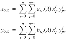 where the wavelength dependence is modeled by coefficients linear in wavelength λ as follows:
 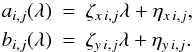 A backward transform is done in the reverse order. At first, the distortion is removed and the paraxial coordinates are calculated
 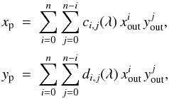 where
where 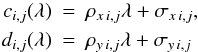 are the backward transform coefficients. Then the input coordinates are
 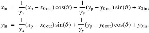 The paraxial description of the optical modules is based on the nominal entrance and exit focal lengths, thereby in a transform between two focal planes, for example, as in the FORE transform, where the coordinates are the positions in the local reference frame in unit of length, the magnification factors γx and γy correspond to the ratio of the focal lengths f,
 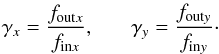 Transforms between a focal plane and a pupil plane (such as the COL transform between the MSA and the GWA) are performed with similar formulas. In this case,
 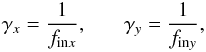 and the output is a vector with a unitary z-component (vx,vy,1). The light path through the dispersive elements of the GWA or the mirror, however, is more easily computed using direction cosines. The expression to convert from the transform result to direction cosines (α,β,γ) is
 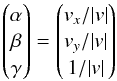 with
with  . The inverse operation to go from direction cosines to the transform coordinates is, therefore,
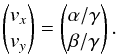
Appendix A.2: Transforms through the GWA elements
When transforming the coordinates of a point in the MSA plane to the FPA plane, one has to take into account the effect of the mirror or the dispersive elements in the GWA on the light path. The specific coordinate transform for a light ray traversing a given element in the GWA (whether the mirror, a grating, or the prism) is applied after having rotated the ray coordinates at the collimator exit to a reference frame with z-axis perpendicular the surface of the given GWA element. If the front surface is tilted by Θy, and the alignment tilt angles are ϑx,ϑy,ϑz, then the first set of rotations applied to the incoming ray iin in direction cosines (αin,βin,γin) is 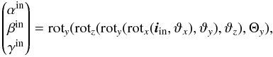 (A.1)where the suffix of the rotation functions denotes the axis around which the rotation is performed. After application of the effect of the GWA element (see below), the outgoing vector iout needs to be rotated back to the GWA output plane (that is CAM entrance plane), using the equation
 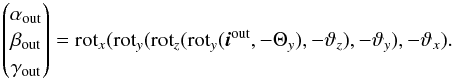 (A.2)The different types of GWA elements are modeled in different ways. In the case of the MIRROR, the light is only reflected, so we have the following wavelength-independent relation
 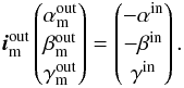 (A.3)For a grating, the chromatic coordinate transform is
 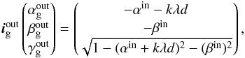 (A.4)where k is the grating order (nominal value in NIRSpec case k = −1) and d is the groove density.
Finally, for a light ray traversing the double-pass prism, the corresponding coordinate transforms are given by the following equations. The prism has a temperature and pressure dependent refraction index n(λ,T,P), so Snell’s refraction law through the front surface is 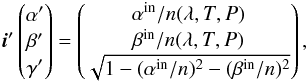 (A.5)followed by the rotation to the reference frame of the prism back surface with the internal prism angle ΘA,
 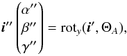 (A.6)the reflection on the back surface
 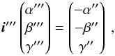 (A.7)going back to the surface frame
 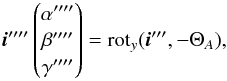 (A.8)and finally Snell’s law through the front surface,
  (A.9)
(A.9)
Appendix A.3: Meeting at the grating
One essential calculation in the extraction process is the derivation of the 2D spectral coordinates (wavelength λ, spatial coordinate in the slit dy) of a certain position on the detector for a certain slit. Unlike the straightforward transform from a slit to detector pixels at a given wavelength, this operation cannot be achieved by simple geometrical transforms in combination with the applicable dispersion law. In an exposure image, where the known parameters are the slit ID and the pixel FPA coordinates, without knowing the wavelength, it is not possible to calculate
the transform at the disperser, and a brute force solution for λ and dy would need a costly iterative optimization for each single point. However, since the coordinate transforms of the COL and CAM optics are achromatic, it is possible to solve for λ and dy with an inverted linear interpolation, and a combination of the individual transforms in the spectrograph.
First, the slit aperture is sampled at its center along the spatial direction with a vector of points extending 5% of the length beyond the edges. This defines a set of coordinates at the MSA. These points are then transformed through the collimator to the GWA plane, and rotated to the disperser surface (just as in the usual transform), giving pairs of two angular coordinates (αin, βin), where βin is primarily depending on dy. On the scale of a single slit, this dependency is approximately linear and an inverted linear interpolation function dy(βin) can be computed. Coming from the other end of the instrument, the pixel coordinates at the FPA are transformed backward through the camera and rotated to the disperser surface, giving two angular coordinates (αout, βout). Since from the dispersion laws βout = −βin, the coordinate dy can be readily determined and, in turn, used to calculate αin with another forward transform from the slit. Finally, the coordinate λ can be computed by inverting the dispersion law. For the grating, this is simply given as  (A.10)where k is the grating order and d is the groove density. For the prism, after computing the value of the refraction index for a number of wavelengths within the nominal wavelength range, an inverted interpolation relation λ(n) can be set up and used to derive the value of λ from the value of n, which is given by
  (A.11)where ΘA is the internal prism angle.
Appendix B: Optical distortions of COL and CAM
Figure B.1 shows the maps of the distortions of COL and CAM as obtained from the model optimization process. Their smoothness and regularity indicates that the optimization process is not driven by individual lines or MOS apertures.
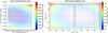 |
Fig. B.1 Map of the optical distortions in the NIRSpec spectrographic part as obtained from the model optimization process. Left: collimator module, plotted in the exit plane. Right: camera module, plotted in the FPA plane. The outline of the two detectors is shown in black. |
All Tables
Summary of the parameters employed in the NIRSpec parametric model of the spectrograph.
Information summary of the type of exposures acquired during NIRSpec testing, which were then used to extract the different type of reference data necessary for the model optimization.
Residuals of the forward projection from MSA to FPA before and after the global model optimization from gratings and the MIRROR on the detector.
Optimized alignment tilt parameters of the gratings relative to the MIRROR surface.
Residuals of calculated trace positions in the spatial direction compared to the measurements extracted with the optimized model.
Residuals of extracted argon emission lines comparing the measured line wavelength with the true wavelength.
Planned updates of the NIRSpec parametric model following major milestones of the JWST project.
All Figures
|
Fig. 1 Paraxial layout of the JWST telescope and NIRSpec optical train with elements at principal planes and the insert for the IFU case. Focal planes are blue; pupil planes are red. |
| In the text | |
|
Fig. 2 Geometrical layout of the MSA projected onto the detector plane. The quadrants Q1–4 contain the microshutters; 5 high-contrast slits and IFU aperture positioned in the horizontal area in the center are indicated. |
| In the text | |
|
Fig. 3 Count-rate image of the two NIRSpec detector arrays (SCA491 and SCA492) of an exposure of the TEST lamp acquired in imaging mode (MIRROR) with the MSA configured in a checkerboard pattern, more clearly visible in the enlargement. SCA491 is on the left (blue side) and SCA492 on the right (red side). The images of the fixed slits are in the center of the images. Areas of defective shutters that fail to open are clearly visible and, in some cases, a full row or column is fully closed. The dark round feature in SCA492 is an area of dead pixels. This image was acquired with the old set of detectors and old MSA module. The image was generated from NIRSpec raw data following the steps described in Sect. 4. |
| In the text | |
|
Fig. 4 Count-rate image of the two NIRSpec detector arrays (SCA491 and SCA492) of an exposure of the argon lamp acquired with G140M and the MSA configured in a dashed slit pattern (see enlargement). In this case the dashed slits were open in Q3 and Q4. The apparent width of the lines depends on the image scaling and blending of unresolved pairs. The regular pattern of spectra is spoiled by the missing spectra due to shutters that fail to open, or by misaligned, overlapping spectra from shutters that cannot be closed (stuck open). The image was generated from NIRSpec raw data using our preprocessing pipeline. |
| In the text | |
|
Fig. 5 Location of spectral reference points in the global model optimization. These reference points consist of the positions of argon emission lines taken with the gratings G140M, G235M, G395M, and G395H. In total, there are 28 020 points distributed over both detectors. The top and bottom groups of green dots are from shutter spectra; the central blue crosses from the fixed slits. |
| In the text | |
|
Fig. 6 Residuals of forward coordinate transforms from MSA to FPA for all of the gratings on the detectors. Left panel: distribution in the detector focal plane. The spectra of the shutters are the wide bands on top and bottom; the stripes in the center are from the fixed slits. Right panel: histograms of residuals in pixels in i and j direction (top, middle) and absolute residuals (bottom). Shown in red are the confidence limits of 68.27% around the median at −0.060 and + 0.062 (i), and at −0.025 and + 0.028 (j), and the limit of 68.27% of absolute residuals (0.071). |
| In the text | |
|
Fig. 7 Residuals of forward coordinate transforms from MSA to FPA for the imaging mode on the detectors. Left panel: distribution in the detector focal plane. The four quadrants of the MSA are clearly visible, the five fixed slits are visible in the center area. Isolated shutters and slits are disturbed by bad pixels, in particular Q3 (top left). Right panel: histograms of residuals in pixels in i and j direction (top, middle) and absolute residuals (bottom). Shown in red are the confidence limits of 68.27% around the median at −0.023 and + 0.022 (i), and at −0.038 and + 0.034 (j), and the limit of 68.27% of absolute residuals (0.046). |
| In the text | |
|
Fig. 8 Combined residuals of the backward transform from FPA to MSA for G140M, G235M, G395M, G395H, and the MIRROR. Top panel: distribution in the MSA plane. The residuals of shutters used in the spectral modes (groups of the dashed slits) vary more strongly than those of the shutters from imaging mode (points spread in the quadrants). The physical direction of the axes are inverted to match the images of the detectors, since the reference frames are not following the optical projection. Bottom panel: histogram of residuals in x and y direction (left, middle) and absolute residuals (right). Shown in red are the confidence limits of 68.27% around the median at −1.84 and 1.98μm (x), and at −1.07 and 1.12μm (y), and the limit of 68.27% of absolute residuals at 2.44μm. |
| In the text | |
|
Fig. 9 Residuals of transforms from IFU slices to FPA with G395H. Left panel: distribution in the detector focal plane. The errors increase toward the lower left, where the CAM distortion was not influenced in the global fit and is not optimal for the IFU, but remain <0.25 px. Right panel: histograms of residuals in pixels in i and j direction (top, middle) and absolute residuals (bottom). Shown in red are the confidence limits of 68.27% around the median at −0.054 and + 0.058 (i), and at −0.004 and + 0.009 (j), and the limit of 68.27% of absolute residuals (0.068). |
| In the text | |
|
Fig. 10 Extraction residuals of the argon lines in the MOS data taken with filter F140X and grating G140H, given in detector pixels. In the main panel, each measured line position from each spectrum is plotted with the error from the fit. The mean residual is −0.019 px with a standard distribution of 0.083 px. The points outside the 4σ-limit of the data are excluded as measurement errors. The right panel shows the distribution of the combined residuals of all lines. |
| In the text | |
|
Fig. B.1 Map of the optical distortions in the NIRSpec spectrographic part as obtained from the model optimization process. Left: collimator module, plotted in the exit plane. Right: camera module, plotted in the FPA plane. The outline of the two detectors is shown in black. |
| In the text | |
Current usage metrics show cumulative count of Article Views (full-text article views including HTML views, PDF and ePub downloads, according to the available data) and Abstracts Views on Vision4Press platform.
Data correspond to usage on the plateform after 2015. The current usage metrics is available 48-96 hours after online publication and is updated daily on week days.
Initial download of the metrics may take a while.