© ESO, 2016

1. Introduction

The best current data, ranging from cosmological to astrophysical scales, have established that the Universe is on average highly homogeneous and isotropic and that it is expanding in an accelerating fashion.

The observation that, in comparison with nearby sources, distance sources (z> 0.3) appear dimmer than predictable in a universe with matter only was interpreted as the need for a dark energy component in the luminosity distance (Riess et al. 1998; Permutter et al. 1999). This dimming, however, could be caused by a variation of any of the other components that affect the luminosity distance, namely by inhomogeneities in the energy densities or anisotropies in the expansion (Amendola et al. 2013). On large scales, the matter distribution is statistically homogeneous. Locally, however, matter is distributed according to a pattern of alternate overdensed regions (filaments) and underdensed regions (voids; Scrimgeour et al. 2012; Watson et al. 2013), which is thought to reflect quantum fluctuations away from homogeneity that originated in the very early Universe. In this paper, we hypothesize that the resulting inhomogeneity in the matter distribution might be imprinted in an angular distribution of the cosmological parameters, which is measured at the scale of the matter distribution pattern, about the average parameter values.

Inhomogeneities in the cosmological parameters distribution might create a dynamical mechanism that would emulate a cosmic acceleration as a derived, instead of fundamental, effect (see e.g. Kolb et al. 2006; Larena et al. 2009; Clarkson & Umeh 2011; Chiesa et al. 2014; Adamek et al. 2015). Conversely, inhomogeneities in the cosmological parameters might reflect new physics, such as a dynamical dark energy component or a modification to the Einstein’s theory of general relativity (see e.g. Amendola et al. 2013). On the one hand, inhomogeneities in the matter distribution might generate fluctuations in the dynamical dark energy, which would imply angular variations of the Hubble parameter across the sky that could be observed as anisotropies of the luminosity distance as a function of redshift d_L(z); on the other hand, fluctuations in the new gravitational fields could have imprints on the local expansion and, consequently, on d_L(z) (Cooray et al. 2010).

Supernovae establish the relation of the luminosity distance with redshift up to z ≈ 1. The luminosity distance is sensitive to both the geometry and growth of structure (Bonvin et al. 2006), which renders supernovae a sensitive probe of the late-time expansion history of the Universe. The current amount of data on SNe from the combination of different SN surveys, if large and homogeneous enough, could be used to investigate the angular distribution of inhomogeneities and hence to investigate the nature of cosmic acceleration.

Supernovae have previously been used to constrain inhomogeneities in the cosmic expansion, namely by measuring the hemispherical anisotropy of H₀ (Kalus et al. 2013), assessing the dependence of H₀ with the position on the cosmic web (Wotjak et al. 2014), mapping {H₀,q₀} in the sky (Bengaly et al. 2015)¹, and by estimating the statistical significance of rejecting an isotropic magnitude-redshift relation (Javanmardi et al. 2015)². Supernovae have also been used to constrain inhomogeneities in the dark energy, namely by constraining fluctuations of dark energy (Blomqvist et al. 2010; Cooray et al. 2010) and by constraining radial inhomogeneity for a Lemaître-Tolman-Bondi metric with a cosmological constant (Valkenburg et al. 2014).

In this paper, we develop a method to probe inhomogeneities in the form of a local estimation of cosmological parameters. We demonstrate the method on type Ia supernovae, in particular by dividing the supernova sample into different regions of the sky and estimating the angular distribution of the cosmological parameters that affect the luminosity distance, namely {Ω_M,Ω_Λ,H₀}, across the different regions. Each region is assumed to be described by a Friedmann-Lemaître-Roberston-Walker metric so that the full sky is an inhomogeneous ensemble of disjoint, locally homogeneous regions. This ensemble of homogeneous regions is an approximate solution to the Einstein equation, which we assume to be a sufficient approximation to enable us to interpret the cosmological parameters {Ω_M,Ω_Λ,H₀} as a description of the true energy content. We also suggest measuring the anisotropy in the angular distribution of the parameters not by looking for particular asymmetries at particular scales, but by computing the angular power spectrum that includes all multipoles accessible in the regions of the sky. We then use the angular fluctuations in H₀ to estimate the backreaction in the sense of Buchert.

Since the Einstein tensor is non-linear in the metric, the average evolution of an inhomogeneous space-time is not the same as the evolution of a smooth space-time with the same initial conditions (Buchert 2000). The effect of inhomogeneities on the average properties is known as backreaction. When averaging over the homogeneous regions, angular fluctuations in the expansion factor, and consequently in H₀, induce a backreaction term in the form of an extra positive acceleration (Räsänen 2006). We derive the analytical extra positive acceleration for a toy model of an arbitrary number of disjoint, homogeneous regions and compute the overall deceleration parameter assuming (a) no backreaction and (b) backreaction for the measured angular distribution of H₀.

This paper is organized as follows. In Sect. 2 we describe the SN data and the theory for the calculation of the observables. In Sect. 3 we introduce the method by performing both a global and a local estimation, according to the parameter estimation described in Appendix A. From the global estimation, there result parameter values taken for fiducial values. From the local estimation, there result maps of the cosmological parameters. In Sect. 4 we include three tests of the inhomogeneity of the SN surveys. The first test is in the SN distribution in redshift, the second test is in the SN distribution in both redshift and sampling, and the third test is in the removal of a noise bias hypothesized as a measure of the inhomogeneity of the SN sampling. We then proceed to analyse the results. In Sect. 5 we compute the power spectrum of the maps of the parameters. In Sect. 6, for a toy model of backreaction, we compute the values of the parameters averaged over the pixels. These are, to the best of our knowledge, the first estimates of inhomogeneities from the angular distribution of cosmological parameters and the first estimates of backreaction effects. In Sect. 7 we discuss current limitations of the method owing to insufficient data and we indicate future research directions.

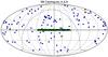Fig. 1 Angular distribution of the JLA type Ia SN sample in celestial coordinates. The sample consists of type Ia SNe compiled from different surveys as described in Betoule et al. (2014). The blue dots indicate low-z data. The green dots indicate SDSS–II data. The yellow dots indicate SNLS data. The red dots indicate HST data. The dashed line represents the Galactic equator.

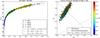Fig. 2 Left panel: distance modulus as a function of redshift. The dots are coloured according to the SN survey and indicate the distance modulus μdata computed from the data on each SN in the sample. The black line indicates the distance modulus μtheo computed theoretically for the values of { ΩM,ΩΛ,H0 } estimated from the complete sample. The black dashed and black dotted lines indicate the distance modulus for two extreme cases: ΩM = 0,ΩΛ = 1 and ΩM = 1,ΩΛ = 0, respectively. Right panel: Markov chain of one realization. The dots indicate the entries in the Markov chain. The position in the graph indicates the values of (ΩM,ΩΛ) of each entry according to the axes, whereas the coloured dots indicate the value of H0 according to the side colour bar. The dashed line represents ΩM + ΩΛ = 1 and the dotted line represents ΩM/ 2−ΩΛ = 0.

2. Supernova data and theory

We use the type Ia supernova sample compiled by the Joint Light-curve Analysis (JLA) SNLS-SDSS collaborative effort (Betoule et al. 2014). The JLA collaboration aimed to include SNe from surveys at different redshifts, improve the accuracy of the calibration, and make the light-curve model uniform across the surveys. The combined sample consists of type Ia SNe from different supernova surveys, namely the Sloan Digital Sky Survey II (SDSS-II) at intermediate redshifts (Sako et al. 2016) and the Supernova Legacy Survey (SNLS) combined with Hubble Space Telescope (HST) surveys at high redshifts and other surveys at low redshifts (Conley et al. 2011), totalling N_SNe = 740 SNe with redshift 0.01 ≤ z ≤ 1.30. The sample includes the SNe in the Hubble flow (z ≥ 0.01) that are not affected by strong Milky Way contamination³. The SNe are distributed on the sky according to Fig. 1.

From the sampled data, we compute the distance modulus for each SN as $\begin{array}{ccc}{\mathit{\mu }}_{\mathrm{data}}\mathrm{\left(}\mathit{z}\mathrm{\right)}\mathrm{=}{\mathit{m}}_{\mathit{B}}\mathrm{\left(}\mathit{z}\mathrm{\right)}\mathrm{-}{\mathit{M}}_{\mathit{B,}\mathrm{eff}}\mathit{.}& & \end{array}$(1)For each SN we take the peak magnitude m_B inferred from the observed magnitude and corrected for the selection bias, and we define the effective absolute magnitude M_B,eff as the absolute magnitude M_B corrected by the time stretching of the light curve x₁ and the supernova colour at maximum brightness c as follows: $\begin{array}{ccc}{\mathit{M}}_{\mathit{B,}\mathrm{eff}}\mathrm{=}{\mathit{M}}_{\mathit{B}}\mathrm{-}\mathit{\alpha }{\mathit{x}}_{\mathrm{1}}\mathrm{+}\mathit{\beta c}\mathit{.}& & \end{array}$(2)The parameters M_B = −19.05 ± 0.02,α = 0.141 ± 0.006, and β = 3.101 ± 0.075 are estimated for all SNe, whereas the parameters { m_B,x₁,c } are estimated for each SN separately by fitting a model of the Ia SN spectral sequence to the photometric data. We compute μ_data for all SNe in the sample and plot it in the left panel of Fig. 2. The error σ_μdata results from the error propagation according to Eqs. (1) and (2) assuming uncorrelated errors.

We now establish the dependence of the distance modulus with the cosmological parameters. The distance modulus is defined in terms of the luminosity distance d_L (measured in Mpc) as $\begin{array}{ccc}{\mathit{\mu }}_{\mathrm{theo}}\mathrm{\left(}\mathit{z}\mathrm{;}{\mathrm{\Omega }}_{\mathrm{M}}\mathit{,}{\mathrm{\Omega }}_{\mathrm{\Lambda }}\mathit{,}{\mathit{H}}_{\mathrm{0}}\mathrm{\right)}\mathrm{=}\mathrm{5}\log \mathrm{\left[}{\mathit{d}}_{\mathrm{L}}\mathrm{\right(}\mathit{z}\mathrm{;}{\mathrm{\Omega }}_{\mathrm{M}}\mathit{,}{\mathrm{\Omega }}_{\mathrm{\Lambda }}\mathit{,}{\mathit{H}}_{\mathrm{0}}\mathrm{\left)}\mathrm{\right]}\mathrm{+}\mathrm{25.}& & \end{array}$(3)For a (3+1)-dimensional line element expressed in spherical coordinates as $\begin{array}{ccc}\mathrm{d}{\mathit{s}}^{\mathrm{2}}\mathrm{=}\mathrm{-}{\mathit{c}}^{\mathrm{2}}\mathrm{d}{\mathit{t}}^{\mathrm{2}}\mathrm{+}{\mathit{a}}^{\mathrm{2}}\mathrm{\left(}\mathit{t}\mathrm{\right)}\left[\frac{\mathrm{d}{\mathit{r}}^{\mathrm{2}}}{\mathrm{1}\mathrm{-}\mathit{\kappa }{\mathit{r}}^{\mathrm{2}}}\mathrm{+}{\mathit{r}}^{\mathrm{2}}{\mathrm{d}}^{\mathrm{2}}{\mathrm{\Omega }}_{\mathrm{\left(}\mathrm{2}\mathrm{\right)}}\right]\mathit{,}& & \end{array}$(4)where κ = { 1,0,−1 } characterizes the spatial curvature and d${}^{\mathrm{2}}\mathrm{\Omega }_{\mathrm{\left(}\mathrm{2}\mathrm{\right)}}\mathrm{\equiv }{\mathrm{d}}^{\mathrm{2}}\mathit{\theta }\mathrm{+}{\sin }^{\mathrm{2}}\mathrm{\left(}\mathit{\theta }\mathrm{\right)}{\mathrm{d}}^{\mathrm{2}}\mathit{\phi }$ stands for the two-sphere line element, the luminosity distance is given by $\begin{array}{ccc}{\mathit{d}}_{\mathrm{L}}\mathrm{\left(}\mathit{z}\mathrm{\right)}\mathrm{=}\frac{{\mathit{a}}_{\mathrm{0}}\mathrm{(}\mathrm{1}\mathrm{+}\mathit{z}\mathrm{)}}{\sqrt{\mathrm{\left|}\mathit{\kappa }\mathrm{\right|}}}{\mathit{S}}_{\mathit{\kappa }}\left[\frac{\mathit{c}\sqrt{\mathrm{\left|}\mathit{\kappa }\mathrm{\right|}}}{{\mathit{a}}_{\mathrm{0}}{\mathit{H}}_{\mathrm{0}}}{\mathrm{\int }}_{\mathrm{0}}^{\mathit{z}}\frac{\mathrm{d}\mathit{z}}{\mathit{E}\mathrm{\left(}\mathit{z}\mathrm{\right)}}\right]\mathit{,}& & \end{array}$(5)where $\begin{array}{ccc}{\mathit{S}}_{\mathit{\kappa }}\mathrm{\left(}\mathit{x}\mathrm{\right)}\mathrm{=}\{\begin{array}{c}\\ & \\ & \\ & \end{array}& & \end{array}$(6)and $\begin{array}{ccc}\mathit{E}\mathrm{\left(}\mathit{z}\mathrm{\right)}\mathrm{=}{\mathrm{[}{\mathrm{\Omega }}_{\mathrm{M}}\mathrm{(}\mathrm{1}\mathrm{+}\mathit{z}{\mathrm{)}}^{\mathrm{3}}\mathrm{+}{\mathrm{\Omega }}_{\mathit{\kappa }}\mathrm{(}\mathrm{1}\mathrm{+}\mathit{z}{\mathrm{)}}^{\mathrm{2}}\mathrm{+}{\mathrm{\Omega }}_{\mathrm{\Lambda }}\mathrm{]}}^{\mathrm{1}\mathit{/}\mathrm{2}}\mathit{,}& & \end{array}$(7)with the dimensionless energy density of matter, curvature, and dark energy at present time given, respectively, by $\begin{array}{ccc}{\mathrm{\Omega }}_{\mathrm{M}}\mathrm{=}\frac{\mathrm{8}\mathit{\pi }{\mathit{G}}_{\mathit{N}}}{\mathrm{3}{\mathit{H}}_{\mathrm{0}}^{\mathrm{2}}}\mathit{\rho ,} {\mathrm{\Omega }}_{\mathit{\kappa }}\mathrm{=}\mathrm{-}\frac{{\mathit{c}}^{\mathrm{2}}\mathit{\kappa }}{{\mathit{a}}_{\mathrm{0}}^{\mathrm{2}}{\mathit{H}}_{\mathrm{0}}^{\mathrm{2}}}\mathit{,} {\mathrm{\Omega }}_{\mathrm{\Lambda }}\mathrm{=}\frac{\mathrm{\Lambda }}{\mathrm{3}{\mathit{H}}_{\mathrm{0}}^{\mathrm{2}}}\mathrm{·}& & \end{array}$(8)Assuming that $\begin{array}{ccc}{\mathrm{\Omega }}_{\mathrm{M}}\mathrm{+}{\mathrm{\Omega }}_{\mathit{\kappa }}\mathrm{+}{\mathrm{\Omega }}_{\mathrm{\Lambda }}\mathrm{=}\mathrm{1}\mathit{,}& & \end{array}$(9)then $\begin{array}{ccc}{\mathit{d}}_{\mathrm{L}}\mathrm{\left(}\mathit{z}\mathrm{\right)}& \mathrm{=}& \frac{\mathit{c}\mathrm{(}\mathrm{1}\mathrm{+}\mathit{z}\mathrm{)}}{\sqrt{\mathrm{\left|}{\mathrm{\Omega }}_{\mathit{\kappa }}\mathrm{\right|}}{\mathit{H}}_{\mathrm{0}}}{\mathit{S}}_{\mathit{k}}[\sqrt{\mathrm{\left|}{\mathrm{\Omega }}_{\mathit{\kappa }}\mathrm{\right|}}\\ & & \end{array}$Hence the distance modulus via the luminosity distance depends on the following set of cosmological parameters { Ω_M,Ω_Λ,H₀ } subject to the condition in Eq. (9).

3. Method

We introduce the method by performing the estimation of the parameters { Ω_M,Ω_Λ,H₀ } as described in Appendix A, first from the complete SN sample and then from SN subsamples grouped by regions in the sky.

3.1. Global parameter estimation

We first use the complete SN sample to fit μ_theo to μ_data and estimate the maximum-likelihood values for the parameters x_i = { Ω_M,Ω_Λ,H₀ } . Whenever unspecified, H₀ is measured in units of km s^-1 Mpc^-1. We ran ten realizations of Markov chains of length 10⁴. The starting point of each realization is randomly generated. We remove the first 20% of entries in the chains to keep the burnt-in phase only. We then thin down the remaining 80% of entries to a half by removing one of each consecutive entry to eliminate correlations within each chain. Averaging over the various realizations of Markov chains, we obtain the following results: ${\mathit{x}}_{\mathit{i}}^{\mathrm{fid}}\mathrm{\equiv }\mathrm{\left\{}{\mathrm{\Omega }}_{\mathrm{M}}^{\mathrm{fid}}\mathit{,}{\mathrm{\Omega }}_{\mathrm{\Lambda }}^{\mathrm{fid}}\mathit{,}{\mathit{H}}_{\mathrm{0}}^{\mathrm{fid}}\mathrm{\right\}}\mathrm{=}\mathrm{\left\{}\mathrm{0.256}\mathit{,}\mathrm{0.715}\mathit{,}\mathrm{71.17}\mathrm{\right\}}\mathrm{\pm }\mathrm{\left\{}\mathrm{0.074}\mathit{,}\mathrm{0.118}\mathit{,}\mathrm{0.44}\mathrm{\right\}}\mathit{.}$ If we moreover impose Ω_M + Ω_Λ = 1, thus enforcing Ω_κ = 0, then we obtain the following results: ${\mathit{x}}_{\mathit{i,}\mathrm{flat}}^{\mathrm{fid}}\mathrm{\equiv }\mathrm{\{}{\mathrm{\Omega }}_{\mathrm{M}}^{\mathrm{fid}}\mathit{,}{\mathrm{\Omega }}_{\mathrm{\Lambda }}^{\mathrm{fid}}\mathit{,}{\mathit{H}}_{\mathrm{0}}^{\mathrm{fid}}{\mathrm{\}}}_{\mathrm{flat}}\mathrm{=}\mathrm{\{}\mathrm{0.267}\mathit{,}\mathrm{0.733}\mathit{,}\mathrm{71.21}\mathrm{\}}\mathrm{\pm }\mathrm{\{}\mathrm{0.018}\mathit{,}\mathrm{0.018}\mathit{,}\mathrm{0.33}\mathrm{\}}\mathit{.}$ (See Table 1.) These are the mean values ${\mathit{x}}_{\mathit{i}}^{\mathrm{fid}}$ and ${\mathit{x}}_{\mathit{i,}\mathrm{flat}}^{\mathrm{fid}}\mathit{,}$ that we use as fiducial values in the subsequent calculations. The errors contain the dispersion in each chain and the dispersion among the averages of the different chains added in quadrature. By fixing H₀ = 70.0 km s^-1 Mpc^-1 and imposing Ω_M + Ω_Λ = 1, we obtain Ω_{M,flat,H0 = 70.0} = 0.322 ± 0.012.

We recall that the JLA collaboration found Ω_M,JLA = 0.295 ± 0.034 for a fixed Hubble parameter H₀ = 70.0 km s^-1 Mpc^-1, which includes our result Ω_{M,flat,H0 = 70.0} within the errors. The results obtained by the JLA collaboration in combination with other data were { Ω_M,Ω_Λ,H₀ } _JLAComb = { 0.305,0.697,68.3 } ± { 0.010,0.010,1.03 } (Betoule et al. 2014). For comparison, in Table 1 we also include the values for these parameters obtained from the ninth-year WMAP data (Hinshaw et al. 2013) and the Planck collaboration (Planck Collaboration XVI 2014). We observe that our results are compatible with the WMAP results, but favour lower values for Ω_M, and simultaneously higher values for Ω_Λ and for H₀, in comparison to the JLAComb and Planck results. In contrast, Riess et al. found H₀ = 73.8 ± 2.4 km s^-1 Mpc^-1 (Riess et al. 2011).

A derived parameter of interest is the curvature energy density Ω_κ, which becomes a dependent variable owing to the flatness condition in Eq. (9). The fiducial values return ${\mathrm{\Omega }}_{\mathit{\kappa }}^{\mathrm{fid}}\mathrm{=}\mathrm{0.029}\mathrm{\pm }\mathrm{0.140}$ and ${\mathrm{\Omega }}_{\mathit{\kappa ,}\mathrm{flat}}^{\mathrm{fid}}\mathrm{=}\mathrm{0.000}\mathrm{\pm }\mathrm{0.026.}$ The values for Ω_κ returned by the above-mentioned studies are included in Table 1. We observe that our results are compatible with the WMAP result but favour values for Ω_κ that are higher than the JLA Comb results and lower than the Planck results.

Another derived parameter of interest is the cosmic deceleration parameter q₀, which is defined in terms of { Ω_M,Ω_Λ } as $\begin{array}{ccc}{\mathit{q}}_{\mathrm{0}}\mathrm{=}\frac{{\mathrm{\Omega }}_{\mathrm{M}}}{\mathrm{2}}\mathrm{-}{\mathrm{\Omega }}_{\mathrm{\Lambda }}\mathrm{=}\mathrm{-}\frac{\mathrm{1}}{{\mathit{H}}_{\mathrm{0}}^{\mathrm{2}}}\frac{\begin{array}{c}\mathrm{¨}\\ \mathit{a}\end{array}}{\mathit{a}}\mathrm{·}& & \end{array}$(12)The fiducial values return ${\mathit{q}}_{\mathrm{0}}^{\mathrm{fid}}\mathrm{=}\mathrm{-}\mathrm{0.586}\mathrm{\pm }\mathrm{0.124}$ and ${\mathit{q}}_{\mathrm{0}\mathit{,}\mathrm{flat}}^{\mathrm{fid}}\mathrm{=}\mathrm{-}\mathrm{0.599}\mathrm{\pm }\mathrm{0.020.}$ The values for q₀ returned by the above-mentioned studies are included in Table 1. We observe that our results are compatible with the WMAP result but favour lower values for q₀ in comparison to the JLAComb and Planck results.

We compute μ_theo for the estimated values ${\mathit{x}}_{\mathit{i}}^{\mathrm{fid}}$ and plot it as a black line in the left panel of Fig. 2. In the right panel of Fig. 2, we plot the Markov chain of one realization. We observe that (a) the points are aligned approximately parallel to the lines of constant H₀ and (b) the points form approximately an ellipse whose largest axis is not parallel to the lines of constant q₀.

To assess the convergence, we apply the Gelman-Rubin heuristic convergence test. For each parameter x_i and N_chain chains, we compute the mean x_ij and variance ${\mathit{\sigma }}_{{\mathit{x}}_{\mathit{ij}}}^{\mathrm{2}}$ of each chain j. We take the mean of all chains and compute the variance of the means of the chains ${\mathit{\sigma }}_{\mathit{x̅}{}_{\mathit{i}}}^{\mathrm{2}}\mathrm{=}{\mathit{\sigma }}^{\mathrm{2}}\mathrm{(}{\mathit{x}}_{\mathit{ij}}\mathrm{about}\mathit{x̅}{}_{\mathit{i}}\mathrm{)}\mathit{.}$ We compute the average of the variances of the chains $\mathit{\sigma ̅}\begin{array}{c}\mathrm{2}\\ \mathit{i}\end{array}\mathrm{=}⟨{\mathit{\sigma }}_{{\mathit{x}}_{\mathit{ij}}}^{\mathrm{2}}{⟩}_{\mathit{j}}\mathit{,}$ and compare with ${\mathit{\sigma }}_{\mathit{x̅}{\mathit{i}}_{}}^{\mathrm{2}}$ forming the ratio $\begin{array}{ccc}{\mathit{r}}_{\mathrm{GR}}\mathrm{=}\frac{\frac{{\mathit{N}}_{\mathrm{chain}}\mathrm{-}\mathrm{1}}{{\mathit{N}}_{\mathrm{chain}}}{\mathit{\sigma }}_{\mathit{x̅}\mathit{i}}^{\mathrm{2}}\mathrm{+}\frac{\mathrm{1}}{{\mathit{N}}_{\mathrm{chain}}}\mathit{\sigma ̅}\begin{array}{c}\mathrm{2}\\ \mathit{i}\end{array}}{{\mathit{\sigma }}_{\mathit{x̅}\mathit{i}}^{\mathrm{2}}}\mathrm{·}& & \end{array}$(13)If the chains are well mixed and have all sampled the parameter space well, then r_GR ~ 1. We find r_GR ≈ 0.90 for the estimation of both ${\mathit{x}}_{\mathit{i}}^{\mathrm{fid}}$ and ${\mathit{x}}_{\mathit{i,}\mathrm{flat}}^{\mathrm{fid}}\mathit{.}$

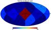Fig. 3 Angular distribution of the number of type Ia SNe per pixel. The total SN sample is divided into subsamples grouped by pixels in the HEALPix pixelation scheme. The number of SNe in each pixel is printed in the centre of the pixel. The pixel indices { 1, 2, 3, 4, 5, 6, 7, 8, 9, 10, 11, 12 } correspond to the SN counts { 15, 14, 95, 7, 380, 38, 70, 26, 10, 6, 6, 73 } . The dashed line represents the Galactic equator.

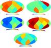Fig. 4 Angular distribution of the estimated parameters { ΩM,ΩΛ,H0 } k,cosmic_var and the derived parameters Ωκ and q0 at each pixel k. The subsample of type Ia SNe in each pixel is used to estimate the value of the parameters { ΩM,ΩΛ,H0 } in that pixel, resulting in a map for each parameter. Operating the estimated maps, results in the derived maps for Ωκ and q0. Subtracting the fiducial values, results in corresponding difference maps. The fiducial values are $\mathrm{\left\{}{\mathrm{\Omega }}_{\mathrm{M}}^{\mathrm{fid}}\mathit{,}{\mathrm{\Omega }}_{\mathrm{\Lambda }}^{\mathrm{fid}}\mathit{,}{\mathit{H}}_{\mathrm{0}}^{\mathrm{fid}}\mathrm{\right\}}\mathrm{=}\mathrm{\left\{}\mathrm{0.256}\mathit{,}\mathrm{0.715}\mathit{,}\mathrm{71.17}\mathrm{\right\}}\mathit{,}$${\mathrm{\Omega }}_{\mathit{\kappa }}^{\mathrm{fid}}\mathrm{=}\mathrm{0.029}\mathit{,}$ and ${\mathit{q}}_{\mathrm{0}}^{\mathrm{fid}}\mathrm{=}\mathrm{-}\mathrm{0.586.}$

3.2. Local parameter estimation: cosmic variance

We proceed to divide the SNe into subsamples grouped by regions in the sky. From each subsample, we aim to estimate the parameters x_i = { Ω_M,Ω_Λ,H₀ } and produce maps such that the values in each region are given by the values of the parameters estimated with the subsample in that region. Hence we must guarantee that the regions have the same surface area and all contain SNe. Ideally each pixel should also have a SN subsample that covers a range of z enough to break the degeneracies among the parameters in Eq. (11). We use the HEALPix pixelation scheme to divide the sphere into pixels of equal surface area (Gorski et al. 2005), hence defining the regions as pixels. In the HEALPix pixelation scheme, we select nside= 1, which produces a map divided into npixel= 12 pixels. The number of SNe in each pixel is indicated in Fig. 3. In this description, the complete sample is equivalent to npixel= 1 pixel.

We then use the SN subsample in each pixel to estimate the maximum-likelihood values for the parameters { Ω_M,Ω_Λ,H₀ } . This estimation is performed, as in the case of the complete sample, on realizations of the original SN distribution in redshift and in space, i.e. for the original dependence of redshift with the position and for the original sampling per pixel. The variance of the estimation in each pixel determines the accuracy with which we can measure the parameters with this sample. For this reason we call this estimation “Cosmic variance”. In each pixel, we ran 30 realizations of Markov chains of length 10⁴. In each pixel, the starting point of each realization is randomly generated as for the case of the complete sample. Also, as in the complete sample, we perform the burnt-in selection and the thinning reduction of the Markov chains in each pixel. Hence from each chain j, at each pixel k, we obtain an estimate for each parameter x_i. The parameter estimation results in maps x_ijk = { Ω_M,Ω_Λ,H₀ } _jk. We average the maps of each parameter over the chains by taking the mean weighted by the number of SNe in each pixel, Since the number of SNe in each pixel is the same for the different chains, this averaging is equivalent to the simple mean of the maps by pixel. We denote the resulting mean maps of the parameters by To assess the convergence, we compute the Gelman–Rubin ratio, finding r_GR ≈ 0.90 for the estimation of all parameters at all pixels.

For better visualization, we compute difference maps $\mathrm{\Delta }\mathit{x̅}{}_{\mathit{ik}}\mathrm{=}\mathit{x̅}{}_{\mathit{ik}}\mathrm{-}{\mathit{x}}_{\mathit{i}}^{\mathrm{fid}}$ by subtracting the fiducial values $\mathrm{\left\{}{\mathrm{\Omega }}_{\mathrm{M}}^{\mathrm{fid}}\mathit{,}{\mathrm{\Omega }}_{\mathrm{\Lambda }}^{\mathrm{fid}}\mathit{,}{\mathit{H}}_{\mathrm{0}}^{\mathrm{fid}}\mathrm{\right\}}$ off the corresponding maps { Ω_M,Ω_Λ,H₀ } _{k,cosmic_var}. Averaging over the various realizations of Markov chains at each pixel, we obtain the difference maps shown in Fig. 4. Similarly, using the maps obtained in the “Cosmic variance” estimation, we compute the maps for Ω_κ and q₀. The difference maps ΔΩ_κ and Δq₀, obtained by subtracting ${\mathrm{\Omega }}_{\mathit{\kappa }}^{\mathrm{fid}}$ and ${\mathit{q}}_{\mathrm{0}}^{\mathrm{fid}}$, respectively, from the corresponding maps, are shown Fig. 4. Comparing the difference maps with the fiducial values, we measure fluctuations of order 10–100% for Ω_M, 1–30% for Ω_Λ, and up to 3% for H₀. Similarly, we measure fluctuations of order 0.1–1000% for Ω_κ and of order 10–60% for q₀. Although the fluctuations of Ω_κ are mostly small, they assume very high values in the pixels where { Ω_M,Ω_Λ } fluctuate in the same direction. From the difference maps, we observe that the fluctuations in the Ω_M map are predominantly towards values higher than ${\mathrm{\Omega }}_{\mathrm{M}}^{\mathrm{fid}}\mathit{,}$ whereas the fluctuations in the Ω_Λ map are predominantly towards values lower than ${\mathrm{\Omega }}_{\mathrm{\Lambda }}^{\mathrm{fid}}\mathit{.}$ The fluctuations in the H₀ map are equally distributed from lower to higher values than the fiducial.

To compare our results with previous studies, we define the largest fluctuation in the difference maps as $\begin{array}{ccc}\max \mathrm{\left(}\mathrm{\Delta }\mathit{x̅}\mathit{ik}\mathrm{\right)}\mathrm{\equiv }\max \mathrm{\left(}\mathit{x̅}\mathit{ik}\mathrm{\right)}\mathrm{-}\min \mathrm{\left(}\mathit{x̅}\mathit{ik}\mathrm{\right)}\mathit{,}& & \end{array}$(14)which yields max( { ΔΩ_M,ΔΩ_Λ,ΔH₀ } ) = { 0.352,0.286,3.84 } ,max(ΔΩ_κ) = 0.363, and max(Δq₀) = 0.452. We recall the results obtained in other SN studies. Kalus et al. found 2.0 <max(ΔH₀)<3.4 km s^-1 Mpc^-1 from the Union 2 data for fixed q₀ = −0.601 (Kalus et al. 2013). Bengaly et al. found max(ΔH₀) = { 4.6,5.6 } km s^-1 Mpc^-1 and max(Δq₀) = { 2.56,1.62 } from the Union 2.1 data and JLA data, respectively (Bengaly et al. 2015). Our results for H₀ are intermediate between the previous results, whereas our results for q₀ are more stringent than those of Bengaly et al. Our results for { Ω_M,Ω_Λ } , and subsequently for Ω_κ are, to the best of our knowledge, the first measurements of this kind.

We also observe a mild negative correlation between the number of SNe in each pixel and the fluctuations about the fiducial values, which hints at a poor sampling derived from an inhomogeneous coverage of the sky, both in angular and redshift space, by the SN surveys. This is further supported by the negative correlation between the number of SNe and the standard deviation of the parameters estimated in each pixel. A poor sampling into pixels implies a poor sampling in redshift, which limits the constraint of the degeneracies among the parameters and hence compromises the estimation of the parameters. Figure 5 illustrates these observations. In order to quantify this correlation, we define the correlation between the maps of the parameters and the number of SNe per pixel N_SNk by $\begin{array}{ccc}\mathrm{Corr}\mathrm{\left[}\mathrm{\Delta }\mathit{x̅}\mathit{ik}\mathit{,}{\mathit{N}}_{\mathrm{SN}\mathit{k}}\mathrm{\right]}& \mathrm{=}& \sum _{\mathit{k}}^{\mathrm{Npixel}}\mathrm{(}\mathrm{\Delta }\mathit{x̅}\mathit{ik}\mathrm{-}{⟨\mathrm{\Delta }\mathit{x̅}\mathit{ik}⟩}_{\mathit{k}}\mathrm{)}\mathrm{(}{\mathit{N}}_{\mathrm{SN}\mathit{k}}\mathrm{-}{⟨{\mathit{N}}_{\mathrm{SN}\mathit{k}}⟩}_{\mathit{k}}\mathrm{)}\\ & & \mathrm{\times }\hspace{0.17em}\frac{\mathrm{1}}{\sqrt{{\sum }_{\mathit{k}}^{\mathrm{Npixel}}\mathrm{(}\mathrm{\Delta }\mathit{x̅}\mathit{ik}\mathrm{-}{⟨\mathrm{\Delta }\mathit{x̅}\mathit{ik}⟩}_{\mathit{k}}{\mathrm{)}}^{\mathrm{2}}}}\\ & & \mathrm{\times }\hspace{0.17em}\frac{\mathrm{1}}{\sqrt{{\sum }_{\mathit{k}}^{\mathrm{Npixel}}\mathrm{(}{\mathit{N}}_{\mathrm{SN}\mathit{k}}\mathrm{-}{⟨{\mathit{N}}_{\mathrm{SN}\mathit{k}}⟩}_{\mathit{k}}{\mathrm{)}}^{\mathrm{2}}}}\mathit{,}\end{array}$which takes values in [−1,1] . Similarly, we define the correlation between the sigma maps of the parameters ${\mathit{\sigma }}_{\mathit{x̅}{\mathit{ik}}_{}}$ and the number of SNe per pixel N_SNk. We find N_SNk] = {−0.394,0.397,−0.113 } and N_SNk] = {−0.408,−0.452,−0.328 } . The values of show that the angular variations of H₀ are less sensitive to the number of SNe per pixel than the angular variations of Ω_M or Ω_Λ. The comparison of the values of with the values of shows that the angular variations of the parameters are not as correlated with the number of SNe per pixel as the corresponding standard deviations.

The Galactic plane could contribute a spurious inhomogeneity in the local parameter estimation. However, an inspection of the pixels through which the Galactic plane crosses does not consistently show higher or lower values of the fluctuations to suggest a correlation.

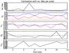Fig. 5 Correlation of the number of SNe per pixel with the fluctuations of the estimated parameters about the fiducial values. At each pixel we plot a) in the first panel, the number of SNe; b) in the second panel, the value of the parameters {ΩM,ΩΛ} as solid red and solid blue lines, respectively, with dashed red and dashed blue lines representing the corresponding fiducial values; c) in the third panel, the standard deviation { σΩM,σΩΛ} as solid red and solid blue lines, respectively; d) in the fourth plot, the value of H0 as a solid black line, with the dashed black line representing the corresponding fiducial value; and e) in the fifth panel, the standard deviation σH0 as a solid black line.

These results are based on the assumption that both μ_data(z) and σ_μdata are independent. The existence of correlations would effectively reduce the number of independent SNe, which would aggravate the parameter estimation in the less SN-populated pixels. Assuming independent errors as a first approximation and having observed that the results are highly affected by the inhomogeneity of the SN surveys, the consideration of correlated errors would be a higher order effect and, hence, safely negligible for the current SN sample.

To assess how the local estimation can be improved, we reduce the number of free parameters by fixing one parameter at a time to the corresponding fiducial value estimated from the complete sample. We observe that the estimation of the Hubble parameter is largely unaffected by the size of the pixel subsample. Conversely the estimation of the energy densities depends highly on the size of the pixel subsample.

4. Inhomogeneity tests

In order to further establish the validity of the method, we perform the following tests of the inhomogeneity of the SN surveys. In the first and second test, following Kalus et al. (2013), we randomize the dependence of the redshift with the position by shuffling the SNe in z. In the first test, we keep the inhomogeneous spatial distribution of the SNe (i.e. we keep the positions of the SNe as in the JLA sample) and, in the second test, we simulate a homogeneous spatial distribution (i.e. we choose random positions for the SNe). In the third test, we hypothesize a noise bias as a measure of the inhomogeneity in the SNe sampling and remove it from the local “Cosmic variance” estimation.

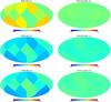Fig. 6 Angular distribution of the parameters { ΩM,ΩΛ,H0 } k,shuffle_sn and { ΩM,ΩΛ,H0 } k,random_pix estimated at each pixel k. The subsample of type Ia SNe in each pixel is used to estimate the value of the parameters in that pixel, which results in a map. Left column: test from shuffling the SNe. Right column: test from randomizing the pixelation. Top panel: difference map $\mathrm{\Delta }{\mathrm{\Omega }}_{\mathrm{M}}\mathrm{=}{\mathrm{\Omega }}_{\mathrm{M}}\mathrm{-}{\mathrm{\Omega }}_{\mathrm{M}}^{\mathrm{fid}}\mathit{.}$Middle panel: difference map $\mathrm{\Delta }{\mathrm{\Omega }}_{\mathrm{\Lambda }}\mathrm{=}{\mathrm{\Omega }}_{\mathrm{\Lambda }}\mathrm{-}{\mathrm{\Omega }}_{\mathrm{\Lambda }}^{\mathrm{fid}}\mathit{.}$Bottom panel: difference map $\mathrm{\Delta }{\mathit{H}}_{\mathrm{0}}\mathrm{=}{\mathit{H}}_{\mathrm{0}}\mathrm{-}{\mathit{H}}_{\mathrm{0}}^{\mathrm{fid}}\mathit{.}$ The fiducial values are $\mathrm{\left\{}{\mathrm{\Omega }}_{\mathrm{M}}^{\mathrm{fid}}\mathit{,}{\mathrm{\Omega }}_{\mathrm{\Lambda }}^{\mathrm{fid}}\mathit{,}{\mathit{H}}_{\mathrm{0}}^{\mathrm{fid}}\mathrm{\right\}}\mathrm{=}\mathrm{\left\{}\mathrm{0.256}\mathit{,}\mathrm{0.715}\mathit{,}\mathrm{71.17}\mathrm{\right\}}\mathit{.}$

4.1. Inhomogeneity test: shuffle the SNe

In this test, we randomize the dependence of redshift with the position for the original sample by shuffling the SNe in z while keeping the positions in the sky. This way, we average out the inhomogeneities in the SN distribution in redshift for the same subsampling per pixel.

Similar to the “Cosmic variance” estimation, we use the SN subsample in each pixel to estimate the maximum-likelihood values for the parameters { Ω_M,Ω_Λ,H₀ } . We call this estimation “Shuffle SNe”. In each pixel, we ran 100 realizations of Markov chains of length 10⁴. For each chain, the SN redshift is randomly shuffled for the same positions. In each pixel, the starting point of each realization is randomly generated as for the case of the complete sample. Also, as in the complete sample, we perform the burnt-in selection and thinning reduction of the Markov chains in each pixel. From each chain, the parameter estimation results in maps x_ijk = { Ω_M,Ω_Λ,H₀ } _{jk,shuffle_sn}. We average the maps for each parameter over the chains. Since the number of SNe in each pixel is the same for the different chains, we average the maps by taking the simple mean by pixel. We denote the resulting mean maps of the parameters by

For better visualization, we compute difference maps by subtracting the fiducial values $\mathrm{\left\{}{\mathrm{\Omega }}_{\mathrm{M}}^{\mathrm{fid}}\mathit{,}{\mathrm{\Omega }}_{\mathrm{\Lambda }}^{\mathrm{fid}}\mathit{,}{\mathit{H}}_{\mathrm{0}}^{\mathrm{fid}}\mathrm{\right\}}$ from the corresponding maps. Averaging over the various realizations of Markov chains at each pixel, we obtain the difference maps shown in the left column of Fig. 6. For an easier comparison, we use the same colour scale for the maps that we used in the “Cosmic variance” estimation.

Comparing the difference maps with $\mathrm{\left\{}{\mathrm{\Omega }}_{\mathrm{M}}^{\mathrm{fid}}\mathit{,}{\mathrm{\Omega }}_{\mathrm{\Lambda }}^{\mathrm{fid}}\mathit{,}{\mathit{H}}_{\mathrm{0}}^{\mathrm{fid}}\mathrm{\right\}}\mathit{,}$ we measure fluctuations of order 1–60% for Ω_M, 1–20% for Ω_Λ, and up to 3% for H₀. We observe that the fluctuations in the Ω_M are predominantly towards values higher than ${\mathrm{\Omega }}_{\mathrm{M}}^{\mathrm{fid}}\mathit{,}$ whereas the fluctuations in the Ω_Λ and H₀ are predominantly towards values lower than the corresponding fiducial values. We also observe the same negative correlation between the number of SNe in each pixel and the fluctuations about the fiducial values as in the “Cosmic variance” estimation.

These fluctuations measure the inhomogeneity in the SN sampling, as observed in Fig. 1, which is reflected in the inhomogeneity of the subsampling into pixels. As observed, increasing the number of realizations increasingly homogenizes the sampling in each pixel and hence reduces the fluctuations about the fiducial values in pixels with large subsamples of SNe; however, increasing the number of realizations does not affect the estimation in pixels with small subsamples of SNe because the cosmic variance is large. For a sufficiently large number of realizations, such that the average is consistent with a homogeneous sampling into pixels with large subsamples of SNe, we hypothesize that this test measures the noise bias in the parameter estimation because of the inhomogeneity of the SN sampling. This noise bias is measured by the average maps produced in this test. Hence by removing this noise bias from the “Cosmic variance” estimation, we would obtain a parameter estimation that is independent of sampling inhomogeneities albeit with increased error.

4.2. Inhomogeneity test: randomize the pixelation

In this test, we randomize the dependence of the redshift with the position for a homogeneous sample per pixel by distributing the SNe in randomly chosen positions in the sky. This way we are averaging out inhomogeneities in the SN distribution in redshift and we simultaneously average out inhomogeneities in the sampling.

Similar to the “Cosmic variance” estimation, we use the SN subsample in each pixel to estimate the maximum-likelihood values for the parameters { Ω_M,Ω_Λ,H₀ } . We call this estimation “Random pixelation”. In each pixel, we ran 100 realizations of Markov chains of length 10⁴. For each chain, the SNe redshift is randomly distributed in a homogeneous way throughout the sky. In each pixel, the starting point of each realization is randomly generated as for the case of the complete sample. Also, as in the complete sample, we perform the burnt-in selection and thinning reduction of the Markov chains in each pixel. From each chain, the parameter estimation results in maps x_ijk = { Ω_M,Ω_Λ,H₀ } _{jk,random_pix}. We average the maps for each parameter over the chains. Since the number of SNe in each pixel varies among the chains, we average the maps by taking the mean weighted by the number of SNe in each pixel. We denote the resulting mean maps of the parameters by .

For better visualization, we compute difference maps by subtracting the fiducial values $\mathrm{\left\{}{\mathrm{\Omega }}_{\mathrm{M}}^{\mathrm{fid}}\mathit{,}{\mathrm{\Omega }}_{\mathrm{\Lambda }}^{\mathrm{fid}}\mathit{,}{\mathit{H}}_{\mathrm{0}}^{\mathrm{fid}}\mathrm{\right\}}$ off the corresponding maps. Averaging over the various realizations of Markov chains at each pixel, we obtain the difference maps { ΔΩ_M,ΔΩ_Λ,ΔH₀ } _{k,random_pix} shown in the right column of Fig. 6.

Comparing the difference maps with $\mathrm{\left\{}{\mathrm{\Omega }}_{\mathrm{M}}^{\mathrm{fid}}\mathit{,}{\mathrm{\Omega }}_{\mathrm{\Lambda }}^{\mathrm{fid}}\mathit{,}{\mathit{H}}_{\mathrm{0}}^{\mathrm{fid}}\mathrm{\right\}}\mathit{,}$ we measure fluctuations of order 10% for Ω_M and Ω_Λ, and of order less than 1% for H₀. These fluctuations measure the limitation of an equal subsampling per pixel of the original sample. Since these fluctuations are smaller than the error of the global parameter estimation, they are consistent with a homogeneous sampling in all pixels, which implies that the original sample is large enough to be divided into subsamples.

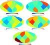Fig. 7 Angular distribution of the estimated parameters { ΩM,ΩΛ,H0 } k,cosmic_var at each pixel k after noise bias removal. The subsample of type Ia SNe in each pixel is used to estimate the value of the parameters { ΩM,ΩΛ,H0 } in that pixel, resulting in a map for each parameter. Subtracting the maps { ΩM,ΩΛ,H0 } k,shuffle_sn averaged over the different realizations, results in the corresponding unbiased maps. Operating the estimated maps results in the derived maps for Ωκ and q0. Subtracting the fiducial values, results in the corresponding difference maps. The fiducial values are $\mathrm{\left\{}{\mathrm{\Omega }}_{\mathrm{M}}^{\mathrm{fid}}\mathit{,}{\mathrm{\Omega }}_{\mathrm{\Lambda }}^{\mathrm{fid}}\mathit{,}{\mathit{H}}_{\mathrm{0}}^{\mathrm{fid}}\mathrm{\right\}}\mathrm{=}\mathrm{\left\{}\mathrm{0.256}\mathit{,}\mathrm{0.715}\mathit{,}\mathrm{71.17}\mathrm{\right\}}\mathit{.}$

4.3. Inhomogeneity test: remove the noise bias

We now proceed to test the hypothesis suggested in the context of the “Shuffle SNe” estimation. We let x_ijk and ${\mathit{x}}_{\mathit{i}{\mathit{j}}^{\mathrm{\prime }}\mathit{k}}^{\mathrm{bias}}$ denote maps produced by j chains of the “Cosmic variance” estimation and j′ chains of the “Shuffle SNe” estimation, respectively. Then for each chain j, we define the unbiased maps as ${\mathit{x}}_{\mathit{ijk}}^{\mathrm{unbias}}\mathrm{\equiv }{\mathit{x}}_{\mathit{ijk}}\mathrm{-}\mathit{x̅}\begin{array}{c}\mathrm{bias}\\ \mathit{ik}\end{array}\mathrm{+}{\mathit{x}}_{\mathit{i}}^{\mathrm{fid}}\mathit{,}$ where $\mathit{x̅}\begin{array}{c}\mathrm{bias}\\ \mathit{ik}\end{array}\mathrm{\equiv }⟨{\mathit{x}}_{\mathit{i}{\mathit{j}}^{\mathrm{\prime }}\mathit{k}}^{\mathrm{bias}}{⟩}_{{\mathit{j}}^{\mathrm{\prime }}}$ is the average over the j′ realizations of the “Shuffle SNe” estimation. The unbiased maps averaged over the chains j are $\mathit{x̅}\begin{array}{c}\mathrm{unbias}\\ \mathit{ik}\end{array}\mathrm{\equiv }⟨{\mathit{x}}_{\mathit{ijk}}{⟩}_{\mathit{j}}\mathrm{-}\mathit{x̅}\begin{array}{c}\mathrm{bias}\\ \mathit{ik}\end{array}\mathrm{+}{\mathit{x}}_{\mathit{i}}^{\mathrm{fid}}\mathit{,}$ and the corresponding unbiased difference maps are $\mathrm{\Delta }\mathit{x̅}\begin{array}{c}\mathrm{unbias}\\ \mathit{ik}\end{array}\mathrm{\equiv }\mathit{x̅}\begin{array}{c}\mathrm{unbias}\\ \mathit{ik}\end{array}\mathrm{-}{\mathit{x}}_{\mathit{i}}^{\mathrm{fid}}\mathit{.}$ We show $\mathrm{\Delta }\mathit{x̅}\begin{array}{c}\mathrm{unbias}\\ \mathit{ik}\end{array}\mathrm{=}\left\{\mathrm{\Delta }{\mathrm{\Omega }}_{\mathrm{M}}\mathit{,}\mathrm{\Delta }{\mathrm{\Omega }}_{\mathrm{\Lambda }}\mathit{,}\mathrm{\Delta }{\mathit{H}}_{\mathrm{0}}\right\}\begin{array}{c}\mathrm{unbias}\\ \mathit{k}\end{array}$ in Fig. 7 to be compared with Fig. 4. Comparing the unbiased difference maps with $\mathrm{\left\{}{\mathrm{\Omega }}_{\mathrm{M}}^{\mathrm{fid}}\mathit{,}{\mathrm{\Omega }}_{\mathrm{\Lambda }}^{\mathrm{fid}}\mathit{,}{\mathit{H}}_{\mathrm{0}}^{\mathrm{fid}}\mathrm{\right\}}\mathit{,}$ we measure fluctuations of order 5–95% for Ω_M, 1–25% for Ω_Λ, and up to 5% for H₀. Similarly, we measure fluctuations of order 35–900% for Ω_κ and 1–50% for q₀.

For the correlations of the number of SNe per pixels with the difference maps and sigma maps, we find $\mathrm{Corr}\mathrm{[}\mathrm{\Delta }\mathit{x̅}\begin{array}{c}\mathrm{unbias}\\ \mathit{ik}\end{array}\mathit{,}$N_SNk] = { −0.117,0.162,−0.343 } and $\mathrm{Corr}\mathrm{\left[}{\mathit{\sigma }}_{\mathit{x̅}\begin{array}{c}\mathrm{unbias}\\ \mathit{ik}\end{array}}\mathit{,}{\mathit{N}}_{\mathrm{SN}\mathit{k}}\mathrm{\right]}\mathrm{=}\mathrm{\{}\mathrm{-}\mathrm{0.653}\mathit{,}\mathrm{-}\mathrm{0.348}\mathit{,}\mathrm{-}\mathrm{0.689}\mathrm{\}}$, respectively. For the unbiased maps in comparison with the original maps, the correlation with the difference maps decreases, whereas the correlation with the error maps increases, as expected. These results seem to indicate the validity of $\mathit{x̅}\begin{array}{c}\mathrm{bias}\\ \mathit{ik}\end{array}$ as a measure of the noise bias from the inhomogeneity of the SN sampling. Figure 8 illustrates these observations to be compared with Fig. 5.

5. Angular power spectrum of the parameters

In order to probe anisotropies in the parameters, we compute the angular power spectrum of the difference maps that result from each realization normalized to the corresponding fiducial parameter. We consider the cosmic variance estimation. For each estimated parameter i, for each realization j, we define the map of the fluctuations about the fiducial value at each pixel k as $\mathit{\delta }{\mathit{x}}_{\mathit{ijk}}\mathrm{=}\mathrm{(}{\mathit{x}}_{\mathit{ijk}}\mathrm{-}{\mathit{x}}_{\mathit{i}}^{\mathrm{fid}}\mathrm{)}\mathit{/}{\mathit{x}}_{\mathit{i}}^{\mathrm{fid}}\mathit{.}$ The map defined over the full sky can be decomposed into spherical harmonics according to $\begin{array}{ccc}\mathit{\delta }{\mathit{x}}_{\mathit{ijk}}\mathrm{\left(}{{n}}_{\mathit{k}}\mathrm{\right)}\mathrm{=}\sum _{\mathit{\ell }\mathrm{=}\mathrm{0}}^{\mathrm{\infty }}\sum _{\mathit{m}\mathrm{=}\mathrm{-}\mathit{\ell }}^{\mathit{\ell }}{\mathit{a}}_{\mathit{\ell m,ij}}{\mathit{Y}}_{\mathit{\ell m}}\mathrm{\left(}{{n}}_{\mathit{k}}\mathrm{\right)}\mathit{,}& & \end{array}$(18)where each pixel k defines a unit direction vector n_k on the sky. The harmonic coefficients are given by $\begin{array}{ccc}{\mathit{a}}_{\mathit{\ell m,ij}}\mathrm{=}\mathrm{\int }\mathrm{d}{\mathrm{\Omega }}_{\mathit{k}}\mathit{\delta }{\mathit{x}}_{\mathit{ijk}}\mathrm{\left(}{{n}}_{\mathit{k}}\mathrm{\right)}{\mathit{Y}}_{\mathit{\ell m}}^{\mathrm{\ast }}\mathrm{\left(}{{n}}_{\mathit{k}}\mathrm{\right)}\mathit{,}& & \end{array}$(19)which for a pixelated map with N_pix pixels can be estimated by $\begin{array}{ccc}\mathit{â}\mathit{\ell m,ij}\mathrm{=}\frac{\mathrm{4}\mathit{\pi }}{{\mathit{N}}_{\mathrm{pixel}}}\sum _{\mathit{k}\mathrm{=}\mathrm{1}}^{{\mathit{N}}_{\mathrm{pixel}}}\mathit{\delta }{\mathit{x}}_{\mathit{ijk}}{\mathit{Y}}_{\mathit{\ell m}}^{\mathrm{\ast }}\mathrm{\left(}{{n}}_{\mathit{k}}\mathrm{\right)}\mathit{.}& & \end{array}$(20)Assuming statistical isotropy, the â_ℓm,ij can be used to estimate the power spectrum Ĉ_ℓ,ij according to $\begin{array}{ccc}⟨{\mathit{a}}_{\mathit{\ell m,ij}}{\mathit{a}}_{{\mathit{\ell }}^{\mathrm{\prime }}{\mathit{m}}^{\mathrm{\prime }}}^{\mathrm{\ast }}⟩\mathrm{=}{\mathit{\delta }}_{\mathit{\ell }{\mathit{\ell }}^{\mathrm{\prime }}}{\mathit{\delta }}_{\mathit{m}{\mathit{m}}^{\mathrm{\prime }}}{\mathit{C}}_{\mathit{\ell ,ij}}\mathit{,}& & \end{array}$(21)which can be inverted to yield the power spectrum of the parameter i from the map realization j$\begin{array}{ccc}\mathit{Ĉ}\mathit{\ell ,ij}\mathrm{=}\frac{\mathrm{1}}{\mathrm{(}\mathrm{2}\mathit{\ell }\mathrm{+}\mathrm{1}\mathrm{)}}\sum _{\mathit{m}\mathrm{=}\mathrm{-}\mathit{\ell }}^{\mathit{\ell }}\mathrm{|}\mathit{â}\mathit{\ell m,ij}{\mathrm{|}}^{\mathrm{2}}\mathit{.}& & \end{array}$(22)The variable ℓ can be written approximately as ℓ = 2π/θ, where θ ranges from the angular size of the map to twice the size of the pixel, which corresponds to the Nyquist frequency. The minimum value of ℓ is determined by the largest scale probed by the map, hence θ = 2π and ℓ_min = 1. Conversely the maximum value of ℓ is determined by the smallest scale probed by the map, hence θ = 2 × (pixelsize) and ℓ_max = 3.

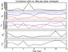Fig. 8 Correlation of the number of SNe per pixel with the estimated parameter fluctuations about the fiducial values after the noise bias removal. At each pixel we plot a) in the first panel, the number of SNe; b) in the second panel, the value of the parameters { ΩM,ΩΛ } as solid red and solid blue lines, respectively, with the dashed red and dashed blue lines representing the corresponding fiducial values; c) in the third panel, the standard deviation { σΩM,σΩΛ } as solid red and solid blue lines, respectively; d) in the fourth plot, the value of H0 as a solid black line, with the dashed black line representing the corresponding fiducial value; e) in the fifth panel, the standard deviation σH0 as a solid black line.

Averaging the power spectra over the different realizations, we obtain the mean power spectrum Ĉ_ℓ,i for the parameters { Ω_M,Ω_Λ,H₀ } _{cosmic_var}$\begin{array}{ccc}\mathit{Ĉ}\mathit{\ell ,i}\mathrm{=}{\mathrm{⟨}\mathit{Ĉ}{\mathit{\ell ,ij}}^{\mathrm{⟩}}}_{\mathit{j}}\mathit{.}& & \end{array}$(23)The variance of the estimator is given by $\begin{array}{ccc}\mathrm{Var}\mathrm{[}\mathit{Ĉ}\mathit{\ell ,i}{\mathrm{]}}^{\mathrm{estimator}}\mathrm{=}\frac{\mathrm{2}}{\mathrm{2}\mathit{\ell }\mathrm{+}\mathrm{1}}\mathit{Ĉ}\begin{array}{c}\mathrm{2}\\ \mathit{\ell ,i}\end{array}\mathit{.}& & \end{array}$(24)Hence the total variance of Ĉ_ℓ,i is the sum of the sample variance about the mean value and the variance of the estimator $\begin{array}{ccc}\mathrm{Var}\mathrm{\left[}\mathit{Ĉ}\mathit{\ell ,i}\mathrm{\right]}\mathrm{=}\mathrm{Var}\mathrm{[}\mathit{Ĉ}\mathit{\ell ,i}{\mathrm{]}}^{\mathrm{sample}}\mathrm{+}\mathrm{Var}\mathrm{[}\mathit{Ĉ}\mathit{\ell ,i}{\mathrm{]}}^{\mathrm{estimator}}\mathit{.}& & \end{array}$(25)The resulting power spectra are plotted in Fig. 9 as dashed lines.

For the density parameters, as well as for the deceleration parameter, we observe that the power spectrum has a maximum at the quadrupole (ℓ = 2). The Ω_M power spectrum is significantly larger than the Ω_Λ power spectrum over all scales, ranging from 5 to 20 times larger. For the Hubble parameter, the power spectrum always increases with the multipole. The quadrupole is approximately { 2.0,1.6,5.4 } times the dipole (ℓ = 1) in the { Ω_M,Ω_Λ,H₀ } _{cosmic_var} power spectra, respectively.

In Bengaly et al. (2015), the dipole was the dominant scale of the H₀ power spectrum produced from the low-redshift (z ≤ 0.20) SNe of the JLA sample. This effect was attributed either to the bulk motion (i.e. the recessional velocity component due to the global expansion) or to the inhomogeneous distribution of the data set.

In order to establish the validity of the method for the power spectrum analysis, we use the average “Shuffle SNe” estimation over j′ realizations, denoted by $\mathit{x̅}\begin{array}{c}\mathrm{bias}\\ \mathit{ik}\end{array}\mathit{,}$ as a measure of the noise bias due to the inhomogeneity of the SN sampling. For each estimated parameter i, we define the average map of the fluctuations about the fiducial value at each pixel k as $\mathit{\delta }\mathit{x̅}\begin{array}{c}\mathrm{bias}\\ \mathit{ik}\end{array}\mathrm{=}\mathrm{(}\mathit{x̅}\begin{array}{c}\mathrm{bias}\\ \mathit{ik}\end{array}\mathrm{-}{\mathit{x}}_{\mathit{i}}^{\mathrm{fid}}\mathrm{)}\mathit{/}{\mathit{x}}_{\mathit{i}}^{\mathrm{fid}}\mathit{.}$ From the decomposition into spherical harmonics of $\mathit{\delta }\mathit{x̅}\begin{array}{c}\mathrm{bias}\\ \mathit{ik}\end{array}\mathit{,}$ we compute $\mathit{Ĉ}\begin{array}{c}\mathrm{bias}\\ \mathit{\ell ,i}\end{array}\mathit{.}$ We define the unbiased power spectrum as $\begin{array}{ccc}\mathit{Ĉ}\begin{array}{c}\mathrm{unbias}\\ \mathit{\ell ,i}\end{array}\mathrm{=}\mathit{Ĉ}\mathit{\ell ,i}\mathrm{-}\mathit{Ĉ}\begin{array}{c}\mathrm{bias}\\ \mathit{\ell ,i}\end{array}& & \end{array}$(26)with total variance $\begin{array}{ccc}\mathrm{Var}\mathrm{\left[}\mathit{Ĉ}\begin{array}{c}\mathrm{unbias}\\ \mathit{\ell ,i}\end{array}\mathrm{\right]}\mathrm{=}\mathrm{Var}\mathrm{\left[}\mathit{Ĉ}\mathit{\ell ,i}\mathrm{\right]}\mathrm{+}\mathrm{Var}\mathrm{[}{\mathit{Ĉ}\mathit{\ell ,i}}^{\mathrm{bias}}{\mathrm{]}}^{\mathrm{estimator}}\mathit{.}& & \end{array}$(27)The resulting power spectra are plotted in Fig. 9 with the bias power spectra as dotted lines and the unbiased power spectra as solid lines. The unbiased power spectra of the density parameters and of the Hubble parameter have the same behaviour, albeit less pronounced, as the corresponding power spectra before the noise bias removal. The exception is the deceleration parameter whose subtle maximum at ℓ = 2 is erased with the noise bias removal. After the noise bias removal, the quadrupole is approximately { 1.3,1.4,5.1 } times the dipole in the { Ω_M,Ω_Λ,H₀ } _{cosmic_var} power spectra, respectively. Although these results seem to indicate the validity of $\mathit{Ĉ}\begin{array}{c}\mathrm{bias}\\ \mathit{\ell ,i}\end{array}$ as a measure of the noise bias and the dominance of the quadrupole as the presence an inhomogeneity scale, the errors are too large to validate the measurements, thus rendering the results compatible with a flat spectrum.

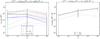Fig. 9 Power spectrum of the parameters estimated from the JLA type Ia SN sample. The dashed lines represent the average power spectra from the cosmic variance estimation, the dotted lines represent the power spectra of the average shuffle SNe estimation, and the solid lines are the unbiased power spectra defined as the difference between the former two. Left panel: power spectra of the matter energy density ΩM and dark energy density ΩΛ (estimated parameters), curvature energy density Ωκ, and the deceleration parameter q0 (derived parameters). Right panel: power spectrum of the Hubble parameter H0 (estimated parameter).

6. Average over the local estimations

We proceed to compute average values of the parameters from the corresponding locally estimated values. We use the maps obtained in the “Cosmic variance” estimation. Given the mean maps over the chains , we want to average the map of each parameter over the pixel subsamples.

One way of averaging consists in taking the mean weighted by the inverse of the variance of the parameter in each pixel k,$\begin{array}{ccc}\mathit{x̅}\mathit{i}\mathrm{=}⟨\mathit{x̅}\mathit{ik}{⟩}_{\mathit{k}}\mathrm{=}\frac{{\sum }_{\mathit{k}}^{{\mathit{N}}_{\mathrm{pixel}}}{\mathit{w}}_{\mathit{k}}\mathit{x̅}\mathit{ik}}{{\sum }_{\mathit{k}}^{{\mathit{N}}_{\mathrm{pixel}}}{\mathit{w}}_{\mathit{k}}}\mathrm{·}& & \end{array}$(28)For the estimated parameters, we find $\mathrm{\left\{}{\overline{\mathrm{\Omega }}}_{\mathrm{M}}\mathit{,}{\overline{\mathrm{\Omega }}}_{\mathrm{\Lambda }}\mathit{,}{\overline{\mathit{H}}}_{\mathrm{0}}\mathrm{\right\}}\mathrm{=}\mathrm{\{}\mathrm{0.242}\mathit{,}$0.607,71.06 } ± { 0.099,0.115,0.87 } and $\mathrm{\{}{\overline{\mathrm{\Omega }}}_{\mathrm{M}}\mathit{,}{\overline{\mathrm{\Omega }}}_{\mathrm{\Lambda }}\mathit{,}{\overline{\mathit{H}}}_{\mathrm{0}}{\mathrm{\}}}_{\mathrm{flat}}\mathrm{=}\mathrm{\{}\mathrm{0.276}\mathit{,}$0.724,70.93 } ± { 0.041,0.041,0.64 } . These values are consistent with, but systematically smaller than, the fiducial values estimated from the complete sample (see Table 2). After the noise bias removal, we find $\mathrm{\{}{\overline{\mathrm{\Omega }}}_{\mathrm{M}}\mathit{,}{\overline{\mathrm{\Omega }}}_{\mathrm{\Lambda }}\mathit{,}{\overline{\mathit{H}}}_{\mathrm{0}}{\mathrm{\}}}_{\mathrm{unbias}}\mathrm{=}\mathrm{\{}\mathrm{0.294}\mathit{,}\mathrm{0.679}\mathit{,}\mathrm{71.37}\mathrm{\}}\mathrm{\pm }${ 0.115,0.120,0.94 } and $\mathrm{\{}{\overline{\mathrm{\Omega }}}_{\mathrm{M}}\mathit{,}{\overline{\mathrm{\Omega }}}_{\mathrm{\Lambda }}\mathit{,}{\overline{\mathit{H}}}_{\mathrm{0}}{\mathrm{\}}}_{\mathrm{unbias,flat}}\mathrm{=}\mathrm{\{}\mathrm{0.256}\mathit{,}\mathrm{0.715}\mathit{,}$71.17 } ± { 0.056,0.056,0.90 } . These values are consistent with the fiducial values. We also observe that the flatness condition yields a lower H₀ than in the absence of the flatness condition, which is the opposite trend of that observed in the estimation from the complete sample.

Similarly, we compute the pixel average of the maps for Ω_κ and q₀ derived from the maps obtained in the “Cosmic variance” estimation. The average value of Ω_κ over the pixels is ${\overline{\mathrm{\Omega }}}_{\mathit{\kappa }}\mathrm{=}\mathrm{0.078}\mathrm{\pm }\mathrm{0.131}$ and ${\overline{\mathrm{\Omega }}}_{\mathit{\kappa ,}\mathrm{flat}}\mathrm{=}\mathrm{0.000}\mathrm{\pm }\mathrm{0.058}\mathit{,}$ and after the noise bias removal it is ${\overline{\mathrm{\Omega }}}_{\mathit{\kappa ,}\mathrm{unbias}}\mathrm{=}\mathrm{0.002}\mathrm{\pm }\mathrm{0.135}$ and ${\overline{\mathrm{\Omega }}}_{\mathit{\kappa ,}\mathrm{unbias,flat}}\mathrm{=}$0.029 ± 0.079. The average value of q₀ over the pixels is and and after the noise bias removal it is and (see Table 2). After the noise bias removal, the pixel average values of both Ω_κ and q₀ become closer to the corresponding values estimated from the complete sample. We also observe that the flatness condition yields a smaller q₀.

Since we are averaging over inhomogeneous maps, we consider a toy model of an inhomogeneous space-time consisting of disjoint, locally homogeneous regions with different expansion factors. Hence another way of averaging consists in taking the mean weighted by the 3-volume V_k of each pixel k,$\begin{array}{ccc}\mathit{x̅}\mathit{i}\mathrm{=}⟨\mathit{x̅}\mathit{ik}{⟩}_{{\mathit{V}}_{\mathit{k}}}\mathrm{=}\frac{{\sum }_{\mathit{k}}^{{\mathit{N}}_{\mathrm{pixel}}}{\mathit{V}}_{\mathit{k}}\mathit{x̅}\mathit{ik}}{{\sum }_{\mathit{k}}^{{\mathit{N}}_{\mathrm{pixel}}}{\mathit{V}}_{\mathit{k}}}\mathrm{·}& & \end{array}$(29)This averaging requires a choice of time slice. Since all pixels have the same surface area and hence the angular directions expand the same way today, we can assume that the radial direction also expands the same way today, which implies that the three-volume is the same today for all pixels. This amounts to identifying a volume as a pixel. Defining v_k = V_k/ ∑ _kV_k and generalizing the result in Räsänen (2006) for N_pixel disjoint regions, the average of the Hubble parameter is given by $\begin{array}{ccc}{⟨\frac{\mathit{ȧ}}{\mathit{a}}⟩}_{{\mathit{V}}_{\mathit{k}}}\mathrm{=}\sum _{\mathit{k}}^{{\mathit{N}}_{\mathrm{pixel}}}{\mathit{v}}_{\mathit{k}}\frac{\mathit{ȧ}}{\mathit{a}}\mathrm{·}& & \end{array}$(30)Taking the derivative, it follows that $\begin{array}{ccc}{⟨\frac{\begin{array}{c}\mathrm{¨}\\ \mathit{a}\end{array}}{\mathit{a}}⟩}_{{\mathit{V}}_{\mathit{k}}}\mathrm{=}\sum _{\mathit{k}}^{{\mathit{N}}_{\mathrm{pixel}}}{\mathit{v}}_{\mathit{k}}\frac{\begin{array}{c}\mathrm{¨}\\ \mathit{a}\end{array}}{\mathit{a}}\mathrm{+}\mathrm{2}\sum _{\mathit{k}}^{{\mathit{N}}_{\mathrm{pixel}}}\sum _{\mathit{l}\mathit{>}\mathit{k}}^{{\mathit{N}}_{\mathrm{pixel}}}{\mathit{v}}_{\mathit{k}}{\mathit{v}}_{\mathit{l}}{\left({\mathit{H}}_{\mathrm{0}\mathit{,k}}\mathrm{-}{\mathit{H}}_{\mathrm{0}\mathit{,l}}\right)}^{\mathrm{2}}\mathit{,}& & \end{array}$(31)which decomposes into a linear term in the pixel average of $\mathrm{(}\begin{array}{c}{}_{\mathrm{¨}}\\ \mathit{a}\end{array}\mathit{/}\mathit{a}\mathrm{)}$ and a quadratic term in differences of H₀ between pairs of pixels. The quadratic (backreaction) term generates an acceleration that is due not to regions speeding up locally, but instead to the slower regions becoming less represented in the average. In the absence of the quadratic term, the volume average reduces to the pixel average above. Then the volume average of q₀ becomes $\begin{array}{ccc}{⟨{\mathit{q}}_{\mathrm{0}}⟩}_{{\mathit{V}}_{\mathit{k}}}& \mathrm{=}& \sum _{\mathit{k}}^{{\mathit{N}}_{\mathrm{pixel}}}{\mathit{v}}_{\mathit{k}}{\mathit{q}}_{\mathrm{0}\mathit{,k}}\\ & & \mathrm{-}\frac{\mathrm{2}}{{\left({\sum }_{\mathit{k}}^{{\mathit{N}}_{\mathrm{pixel}}}{\mathit{v}}_{\mathit{k}}{\mathit{H}}_{\mathrm{0}\mathit{,k}}\right)}^{\mathrm{2}}}\sum _{\mathit{k}}^{{\mathit{N}}_{\mathrm{pixel}}}\sum _{\mathit{l}\hspace{0.17em}\mathit{>}\hspace{0.17em}\mathit{k}}^{{\mathit{N}}_{\mathrm{pixel}}}{\mathit{v}}_{\mathit{k}}{\mathit{v}}_{\mathit{l}}{\left({\mathit{H}}_{\mathrm{0}\mathit{,k}}\mathrm{-}{\mathit{H}}_{\mathrm{0}\mathit{,l}}\right)}^{\mathrm{2}}\mathit{.}\end{array}$Using the fluctuations in H₀ measured in the local parameter estimation, we find and and after the noise bias removal we find and (see Table 2). After the noise bias removal, the volume average values become closer to the value for the deceleration estimated from the complete sample. The results from both averaging methods strengthen the validity of $\mathit{x̅}\begin{array}{c}\mathrm{bias}\\ \mathit{ik}\end{array}$ as a measure of the noise bias due to the inhomogeneity of the SN sampling.

The quadratic term is of order 10^-3 (or lower) times the linear term, which means that the error of the difference is below the standard deviation. Hence for the angular fluctuations in H₀ measured with this SN sample, the contribution of the quadratic term in Eq. (31) is insignificant, which renders the volume averaging equivalent to the pixel averaging. Hence in the context of this toy model of an inhomogeneous space-time, backreaction is not a viable dynamical mechanism to emulate cosmic acceleration.

7. Conclusions

In this paper, we developed a method to probe the inhomogeneity of the large-scale structure and cosmic acceleration and applied to type Ia SN data. In particular, we subsampled the original SN sample into pixels of equal surface area and in each pixel we estimated the cosmological parameters that affect the luminosity distance, namely { Ω_M,Ω_Λ,H₀ } , assuming a local Friedmann-Lemaître-Roberston-Walker metric in each pixel. This local parameter estimation resulted in maps of the cosmological parameters with the same pixelation as the SN subsamples.

We measured fluctuations about the average values of order 5–95% for the matter energy density Ω_M, 1–25% for the dark energy density Ω_Λ, and to 5% for the Hubble parameter H₀, which translate into fluctuations about the average values of order 35–900% for the curvature energy density Ω_κ and 1–50% for the deceleration parameter q₀. The comparison of our results with those obtained in other SN studies indicates convergence of the results and consistency among the measurements. Owing to the spatial inhomogeneity of the SN surveys, as demonstrated by the tests performed, the pixel subsamples are statistically unequal. As a result, well-sampled pixels return robust estimations, whereas poorly sampled pixels return weak constraints. We also assessed how the local estimation can be improved by fixing one parameter. From this test, we observed that the estimation of H₀ is largely unaffected by the size of the pixel subsample, whereas the estimation of the energy densities depends highly on the size of the pixel subsample. For more robust results on { Ω_M,Ω_Λ } , and subsequently on Ω_κ, we would need a SN survey that covered the sky more homogeneously so that all pixels were sufficiently sampled both in number of supernovae and in redshift range.

We also computed the power spectrum of the corresponding maps of the parameters. As a result of the size of each pixel, which was selected so that all pixels contained SNe, the largest multipole accessible is the octopole ℓ = 3. Previous measurements were aimed at the measurement of the dipole ℓ = 1 only.

For an analytical toy model of an inhomogeneous ensemble of homogeneous pixels, we derived the backreaction term in the deceleration parameter due to the fluctuations of H₀ across the sky. The overall deceleration parameter, computed as the average over the pixels assuming (a) no backreaction and (b) backreaction, results in a difference of order 10^-3 between the two averaging methods. This means that, for the toy model considered, the backreaction generates insignificant extra acceleration.

This paper is a proof of concept to measure deviations from homogeneity. Despite the limitations of the SN data available to date, we demonstrated that this method can measure deviations from homogeneity in the cosmological parameters across the sky. Investigating the averaging variability can be relevant to look for a dynamical mechanism that emulates a cosmic acceleration as a derived, instead of fundamental, effect. An idea worth exploring would be to repeat the local estimation for the

dependence of other parameters without an a priori dark energy component, for example using a kinematic parametrization of the luminosity distance expressed in terms of time derivatives of the scale factor. Investigating the angular distribution of the parameters can also be relevant to characterize the pattern of overdensed regions (filaments) and underdensed regions (voids) observed on large scales. Another idea worth exploring would be to correlate the angular distribution of the cosmological parameters with probes of the large-scale structure from which a pattern of matter distribution might emerge. Yet another idea would be to use the σ₈–H₀ degeneracy to explore the implications of the angular variation of the cosmic expansion to neutrino physics (∑ m_ν or N_eff).

Further investigation along these lines can be important for the formulation and validation of inhomogeneous models on the basis of an unprecedented amount of data that we anticipate having in the near future.

Acknowledgments

The authors thank I. Hooke, V. Marra, N. Nunes, and S. Räsänen for useful discussions. CSC is funded by Fundação para a Ciência e a Tecnologia (FCT), Grant No. SFRH/BPD/65993/2009.

References

Appendix A: Estimation method

We aim to find the values { Ω_M,Ω_Λ,H₀ } that best fit μ_theo to μ_data. The probability that a given combination of values { Ω_M,Ω_Λ,H₀ } fits the data is known as the posterior probability P_post and is defined as $\begin{array}{ccc}{\mathit{P}}_{\mathrm{post}}\mathrm{\left(}{\mathrm{\Omega }}_{\mathit{M}}\mathit{,}{\mathrm{\Omega }}_{\mathrm{\Lambda }}\mathit{,}{\mathit{H}}_{\mathrm{0}}\mathrm{\right|}\mathrm{\left\{}{\mathit{\mu }}_{\mathrm{data}}\mathrm{\right(}{\mathit{z}}_{\mathit{i}}\mathrm{\left)}\mathrm{\right\}}\mathrm{)}\mathrm{=}\frac{\mathit{P}\mathrm{\left(}\mathrm{\right\{}{\mathit{\mu }}_{\mathrm{data}}\mathrm{\left(}{\mathit{z}}_{\mathit{i}}\mathrm{\right)}\mathrm{\left\}}\mathrm{\right|}{\mathrm{\Omega }}_{\mathit{M}}\mathit{,}{\mathrm{\Omega }}_{\mathrm{\Lambda }}\mathit{,}{\mathit{H}}_{\mathrm{0}}\mathrm{)}}{\mathit{P}\mathrm{\left(}\mathrm{\right\{}{\mathit{\mu }}_{\mathrm{data}}\mathrm{\left(}{\mathit{z}}_{\mathit{i}}\mathrm{\right)}\mathrm{\}}}{\mathit{P}}_{\mathrm{prior}}\mathit{.}& & \end{array}$(A.1)The probability of the data given the values for the model parameters (the numerator) is known as the likelihood, and the integral of the likelihood over the parameters’ space (the denominator) is known as the evidence. The prior probability P_prior describes informed constraints that we impose a priori on the parameters.

We assume that the measurements of μ at the different zs are independent and that the noise is Gaussian as a first approximation. Then the likelihood is given by $\begin{array}{ccc}& & \mathrm{ℒ}\mathrm{\left(}{\mathrm{\Omega }}_{\mathit{M}}\mathit{,}{\mathrm{\Omega }}_{\mathrm{\Lambda }}\mathit{,}{\mathit{H}}_{\mathrm{0}}\mathrm{\right)}\mathrm{\equiv }\mathit{P}\mathrm{\left(}\mathrm{\right\{}{\mathit{\mu }}_{\mathrm{data}}\mathrm{\left(}{\mathit{z}}_{\mathit{i}}\mathrm{\right)}\mathrm{\left\}}\mathrm{\right|}{\mathrm{\Omega }}_{\mathit{M}}\mathit{,}{\mathrm{\Omega }}_{\mathrm{\Lambda }}\mathit{,}{\mathit{H}}_{\mathrm{0}}\mathrm{)}\\ & \mathrm{=}& \frac{\mathrm{1}}{\mathrm{(}\mathrm{2}\mathit{\pi }{\mathrm{)}}^{{\mathit{N}}_{\mathrm{SNe}}\mathit{/}\mathrm{2}}{\mathrm{􏽑}}_{\mathit{i}}^{{\mathit{N}}_{\mathrm{SNe}}}{\mathit{\sigma }}_{{\mathit{\mu }}_{\mathrm{data}}}\mathrm{\left(}{\mathit{z}}_{\mathit{i}}\mathrm{\right)}}\\ & & \mathrm{\times }\exp \left[\mathrm{-}\frac{\mathrm{1}}{\mathrm{2}}\sum _{\mathit{i}}^{{\mathit{N}}_{\mathrm{SNe}}}{\left(\frac{{\mathit{\mu }}_{\mathrm{data}}\mathrm{\left(}{\mathit{z}}_{\mathit{i}}\mathrm{\right)}\mathrm{-}{\mathit{\mu }}_{\mathrm{theo}}\mathrm{\left(}{\mathit{z}}_{\mathit{i}}\mathrm{;}{\mathrm{\Omega }}_{\mathrm{M}}\mathit{,}{\mathrm{\Omega }}_{\mathrm{\Lambda }}\mathit{,}{\mathit{H}}_{\mathrm{0}}\mathrm{\right)}}{{\mathit{\sigma }}_{{\mathit{\mu }}_{\mathrm{data}}}\mathrm{\left(}{\mathit{z}}_{\mathit{i}}\mathrm{\right)}}\right)}^{\mathrm{2}}\right]\mathrm{·}\end{array}$

Each combination of values { Ω_M,Ω_Λ,H₀ } _trial is generated from a Gaussian distribution and defines a trial. We implement the Metropolis-Hastings algorithm to produce Markov chains where the samples are generated from the conditional posterior distribution with the following priors: (a) Θ(Ω_M)Θ(Ω_Λ)Θ(H₀) and (b) Θ(1−Ω_M)Θ(1−Ω_Λ), with Θ standing for the Heaviside function. For each trial we define $\begin{array}{ccc}{\mathit{\chi }}_{\mathrm{trial}}^{\mathrm{2}}\mathrm{=}\sum _{\mathit{i}}^{{\mathit{N}}_{\mathrm{SNe}}}{\left(\frac{{\mathit{\mu }}_{\mathrm{data}}\mathrm{\left(}{\mathit{z}}_{\mathit{i}}\mathrm{\right)}\mathrm{-}{\mathit{\mu }}_{\mathrm{theo}}\mathrm{\left(}{\mathit{z}}_{\mathit{i}}\mathrm{;}\mathrm{\right\{}{\mathrm{\Omega }}_{\mathrm{M}}\mathit{,}{\mathrm{\Omega }}_{\mathrm{\Lambda }}\mathit{,}{\mathit{H}}_{\mathrm{0}}{\mathrm{\}}}_{\mathrm{trial}}\mathrm{)}}{{\mathit{\sigma }}_{{\mathit{\mu }}_{\mathrm{data}}}\mathrm{\left(}{\mathit{z}}_{\mathit{i}}\mathrm{\right)}}\right)}^{\mathrm{2}}\mathit{,}& & \end{array}$(A.5)and compare the likelihood between the trial combination and the previous combination by taking the ratio of the corresponding likelihoods times the prior as follows: $\begin{array}{ccc}\mathit{LR}\mathrm{=}\exp \left[\mathrm{-}\frac{\mathrm{1}}{\mathrm{2}}\mathrm{(}{\mathit{\chi }}_{\mathrm{trial}}^{\mathrm{2}}\mathrm{-}{\mathit{\chi }}_{\mathrm{prev}}^{\mathrm{2}}\mathrm{)}\right]\frac{{\mathit{P}}_{\mathrm{prior}}\mathrm{\left(}\mathrm{\right\{}{\mathrm{\Omega }}_{\mathrm{M}}\mathit{,}{\mathrm{\Omega }}_{\mathrm{\Lambda }}\mathit{,}{\mathit{H}}_{\mathrm{0}}{\mathrm{\}}}_{\mathrm{trial}}\mathrm{)}}{{\mathit{P}}_{\mathrm{prior}}\mathrm{\left(}\mathrm{\right\{}{\mathrm{\Omega }}_{\mathrm{M}}\mathit{,}{\mathrm{\Omega }}_{\mathrm{\Lambda }}\mathit{,}{\mathit{H}}_{\mathrm{0}}{\mathrm{\}}}_{\mathrm{prev}}\mathrm{)}}\mathrm{·}& & \end{array}$(A.6)If the ratio is larger than one, then the trial combination is accepted and added to the chain. Otherwise, the ratio is compared with a trial from a uniform distribution defined in [0,1] , and if the ratio is larger, then the trial combination is accepted and added to the chain; otherwise, the trial combination is rejected and the previous combination is added to the chain instead.

All Tables

All Figures

	Fig. 1 Angular distribution of the JLA type Ia SN sample in celestial coordinates. The sample consists of type Ia SNe compiled from different surveys as described in Betoule et al. (2014). The blue dots indicate low-z data. The green dots indicate SDSS–II data. The yellow dots indicate SNLS data. The red dots indicate HST data. The dashed line represents the Galactic equator.
In the text

Fig. 2 Left panel: distance modulus as a function of redshift. The dots are coloured according to the SN survey and indicate the distance modulus μdata computed from the data on each SN in the sample. The black line indicates the distance modulus μtheo computed theoretically for the values of { ΩM,ΩΛ,H0 } estimated from the complete sample. The black dashed and black dotted lines indicate the distance modulus for two extreme cases: ΩM = 0,ΩΛ = 1 and ΩM = 1,ΩΛ = 0, respectively. Right panel: Markov chain of one realization. The dots indicate the entries in the Markov chain. The position in the graph indicates the values of (ΩM,ΩΛ) of each entry according to the axes, whereas the coloured dots indicate the value of H0 according to the side colour bar. The dashed line represents ΩM + ΩΛ = 1 and the dotted line represents ΩM/ 2−ΩΛ = 0.

In the text

Fig. 3 Angular distribution of the number of type Ia SNe per pixel. The total SN sample is divided into subsamples grouped by pixels in the HEALPix pixelation scheme. The number of SNe in each pixel is printed in the centre of the pixel. The pixel indices { 1, 2, 3, 4, 5, 6, 7, 8, 9, 10, 11, 12 } correspond to the SN counts { 15, 14, 95, 7, 380, 38, 70, 26, 10, 6, 6, 73 } . The dashed line represents the Galactic equator.

In the text

Fig. 4 Angular distribution of the estimated parameters { ΩM,ΩΛ,H0 } k,cosmic_var and the derived parameters Ωκ and q0 at each pixel k. The subsample of type Ia SNe in each pixel is used to estimate the value of the parameters { ΩM,ΩΛ,H0 } in that pixel, resulting in a map for each parameter. Operating the estimated maps, results in the derived maps for Ωκ and q0. Subtracting the fiducial values, results in corresponding difference maps. The fiducial values are $\mathrm{\left\{}{\mathrm{\Omega }}_{\mathrm{M}}^{\mathrm{fid}}\mathit{,}{\mathrm{\Omega }}_{\mathrm{\Lambda }}^{\mathrm{fid}}\mathit{,}{\mathit{H}}_{\mathrm{0}}^{\mathrm{fid}}\mathrm{\right\}}\mathrm{=}\mathrm{\left\{}\mathrm{0.256}\mathit{,}\mathrm{0.715}\mathit{,}\mathrm{71.17}\mathrm{\right\}}\mathit{,}$${\mathrm{\Omega }}_{\mathit{\kappa }}^{\mathrm{fid}}\mathrm{=}\mathrm{0.029}\mathit{,}$ and ${\mathit{q}}_{\mathrm{0}}^{\mathrm{fid}}\mathrm{=}\mathrm{-}\mathrm{0.586.}$

In the text

Fig. 5 Correlation of the number of SNe per pixel with the fluctuations of the estimated parameters about the fiducial values. At each pixel we plot a) in the first panel, the number of SNe; b) in the second panel, the value of the parameters {ΩM,ΩΛ} as solid red and solid blue lines, respectively, with dashed red and dashed blue lines representing the corresponding fiducial values; c) in the third panel, the standard deviation { σΩM,σΩΛ} as solid red and solid blue lines, respectively; d) in the fourth plot, the value of H0 as a solid black line, with the dashed black line representing the corresponding fiducial value; and e) in the fifth panel, the standard deviation σH0 as a solid black line.

In the text

Fig. 6 Angular distribution of the parameters { ΩM,ΩΛ,H0 } k,shuffle_sn and { ΩM,ΩΛ,H0 } k,random_pix estimated at each pixel k. The subsample of type Ia SNe in each pixel is used to estimate the value of the parameters in that pixel, which results in a map. Left column: test from shuffling the SNe. Right column: test from randomizing the pixelation. Top panel: difference map $\mathrm{\Delta }{\mathrm{\Omega }}_{\mathrm{M}}\mathrm{=}{\mathrm{\Omega }}_{\mathrm{M}}\mathrm{-}{\mathrm{\Omega }}_{\mathrm{M}}^{\mathrm{fid}}\mathit{.}$Middle panel: difference map $\mathrm{\Delta }{\mathrm{\Omega }}_{\mathrm{\Lambda }}\mathrm{=}{\mathrm{\Omega }}_{\mathrm{\Lambda }}\mathrm{-}{\mathrm{\Omega }}_{\mathrm{\Lambda }}^{\mathrm{fid}}\mathit{.}$Bottom panel: difference map $\mathrm{\Delta }{\mathit{H}}_{\mathrm{0}}\mathrm{=}{\mathit{H}}_{\mathrm{0}}\mathrm{-}{\mathit{H}}_{\mathrm{0}}^{\mathrm{fid}}\mathit{.}$ The fiducial values are $\mathrm{\left\{}{\mathrm{\Omega }}_{\mathrm{M}}^{\mathrm{fid}}\mathit{,}{\mathrm{\Omega }}_{\mathrm{\Lambda }}^{\mathrm{fid}}\mathit{,}{\mathit{H}}_{\mathrm{0}}^{\mathrm{fid}}\mathrm{\right\}}\mathrm{=}\mathrm{\left\{}\mathrm{0.256}\mathit{,}\mathrm{0.715}\mathit{,}\mathrm{71.17}\mathrm{\right\}}\mathit{.}$

In the text

Fig. 7 Angular distribution of the estimated parameters { ΩM,ΩΛ,H0 } k,cosmic_var at each pixel k after noise bias removal. The subsample of type Ia SNe in each pixel is used to estimate the value of the parameters { ΩM,ΩΛ,H0 } in that pixel, resulting in a map for each parameter. Subtracting the maps { ΩM,ΩΛ,H0 } k,shuffle_sn averaged over the different realizations, results in the corresponding unbiased maps. Operating the estimated maps results in the derived maps for Ωκ and q0. Subtracting the fiducial values, results in the corresponding difference maps. The fiducial values are $\mathrm{\left\{}{\mathrm{\Omega }}_{\mathrm{M}}^{\mathrm{fid}}\mathit{,}{\mathrm{\Omega }}_{\mathrm{\Lambda }}^{\mathrm{fid}}\mathit{,}{\mathit{H}}_{\mathrm{0}}^{\mathrm{fid}}\mathrm{\right\}}\mathrm{=}\mathrm{\left\{}\mathrm{0.256}\mathit{,}\mathrm{0.715}\mathit{,}\mathrm{71.17}\mathrm{\right\}}\mathit{.}$

In the text

Fig. 8 Correlation of the number of SNe per pixel with the estimated parameter fluctuations about the fiducial values after the noise bias removal. At each pixel we plot a) in the first panel, the number of SNe; b) in the second panel, the value of the parameters { ΩM,ΩΛ } as solid red and solid blue lines, respectively, with the dashed red and dashed blue lines representing the corresponding fiducial values; c) in the third panel, the standard deviation { σΩM,σΩΛ } as solid red and solid blue lines, respectively; d) in the fourth plot, the value of H0 as a solid black line, with the dashed black line representing the corresponding fiducial value; e) in the fifth panel, the standard deviation σH0 as a solid black line.

In the text

Fig. 9 Power spectrum of the parameters estimated from the JLA type Ia SN sample. The dashed lines represent the average power spectra from the cosmic variance estimation, the dotted lines represent the power spectra of the average shuffle SNe estimation, and the solid lines are the unbiased power spectra defined as the difference between the former two. Left panel: power spectra of the matter energy density ΩM and dark energy density ΩΛ (estimated parameters), curvature energy density Ωκ, and the deceleration parameter q0 (derived parameters). Right panel: power spectrum of the Hubble parameter H0 (estimated parameter).

In the text

References

- Adamek, A., Clarkson, C., Durrer, R., & Kunz, M. 2015, Phys. Rev. Lett., 114, 051302 [NASA ADS] [CrossRef] [Google Scholar]
- Amendola, L., Appleby, S., Bacon, D., et al. 2013, Liv. Rev. Relat., 16, 6 [Google Scholar]
- Bengaly, C. A. P., Bernui, A., & Alcaniz, J. S. 2015, ApJ, 808, 39 [NASA ADS] [CrossRef] [Google Scholar]
- Betoule, M., Rodríguez, E., & Amado, P. J. 2014, A&A, 568, A32 [CrossRef] [Google Scholar]
- Blomqvist, M., Enander, J., & Mortsell, E. 2010, JCAP, 10, 018 [NASA ADS] [CrossRef] [Google Scholar]
- Bonvin, C., Durrer, R., & Gasparini, M. A. 2006, Phys. Rev. D, 73, 023523 [NASA ADS] [CrossRef] [Google Scholar]
- Buchert, T. 2000, General Relativity Gravitation, 32, 105 [Google Scholar]
- Chiesa, M., Maino, D., & Majerotto, E. 2014, JCAP, 12, 49 [Google Scholar]
- Clarkson, & Umeh 2011, Classical Quantum Gravity, 28 [Google Scholar]
- Conley, A., Guy, J., Sullivan, M., et al. 2011, ApJS, 192, 1 [NASA ADS] [CrossRef] [EDP Sciences] [Google Scholar]
- Cooray, A., Holz, D. E., & Caldwell, R. 2010, JCAP, 11, 15 [NASA ADS] [CrossRef] [Google Scholar]
- Hinshaw, G., Larson, D., Komatsu, E., et al. 2013, ApJS, 208, 19 [NASA ADS] [CrossRef] [Google Scholar]
- Górski, K. M., Hivon, E., Banday, A. J., et al. 2005, ApJ, 622, 759 [NASA ADS] [CrossRef] [Google Scholar]
- Javanmardi, B., Porciani, C., Kroupa, P., & Pflamm-Altenburg, J. 2015, ApJ, 810, 47 [NASA ADS] [CrossRef] [Google Scholar]
- Kalus, B., Schwarz, D. J., Seikel, M., & Wiegand, A. 2013, A&A, 553, A56 [NASA ADS] [CrossRef] [EDP Sciences] [Google Scholar]
- Kolb, E. W., Matarrese, S., & Riotto, A. 2006, New J. Phys., 8, 322 [NASA ADS] [CrossRef] [Google Scholar]
- Larena, J., Alimi, J. M., Buchert, T., Kunz, M., & Corasaniti, P. S. 2009, Phys. Rev. D, 79, 083011 [NASA ADS] [CrossRef] [Google Scholar]
- Perlmutter, S., Aldering, G., Goldhaber, G., et al. 1999, ApJ, 517, 565 [NASA ADS] [CrossRef] [Google Scholar]
- Planck Collaboration XVI. 2014, A&A, 571, A16 [NASA ADS] [CrossRef] [EDP Sciences] [Google Scholar]
- Räsänen, S. 2006, JCAP, 11, 003 [Google Scholar]
- Riess, A. G., Filippenko, A. V., Challis, P., et al. 1998, AJ, 116, 1009 [NASA ADS] [CrossRef] [Google Scholar]
- Riess, A. G., Macri, L., Casertano, S., et al. 2011, ApJ, 730, 119 [NASA ADS] [CrossRef] [Google Scholar]
- Sako, M., Bassett, B., Becker, A. C., et al. 2016, ApJS, submitted [arXiv:1401.3317] [Google Scholar]
- Scrimgeour, M. I., Davis, T., Blake, C., et al. 2012, MNRAS, 425, 116 [NASA ADS] [CrossRef] [Google Scholar]
- Valkenburg, W., Marra Valerio, & Clarkson, C. 2014, MNRAS, 438, 6 [NASA ADS] [CrossRef] [Google Scholar]
- Watson, W. A., Iliev, I. T., Diego, J. M., et al. 2013, MNRAS, 437, 3776 [NASA ADS] [CrossRef] [Google Scholar]
- Wotjak, R., Knebe, A., Watson, W. A., et al. 2014, MNRAS, 438, 1805 [NASA ADS] [CrossRef] [Google Scholar]