| Issue |
A&A
Volume 592, August 2016
|
|
|---|---|---|
| Article Number | A22 | |
| Number of page(s) | 12 | |
| Section | Extragalactic astronomy | |
| DOI | https://doi.org/10.1051/0004-6361/201628117 | |
| Published online | 06 July 2016 | |
An innovative blazar classification based on radio jet kinematics
1 LUTH, Observatoire de Paris, PSL, CNRS, Université Paris Diderot, 5 place Jules Janssen, 92190 Meudon, France
e-mail: This email address is being protected from spambots. You need JavaScript enabled to view it.
2 Santa Cruz Institute for Particle Physics and Department of Physics, University of California at Santa Cruz, Santa Cruz, CA 95064, USA
Received: 12 January 2016
Accepted: 30 April 2016
Abstract
Context. Blazars are usually classified following their synchrotron peak frequency (νF(ν) scale) as high, intermediate, low frequency peaked BL Lacs (HBLs, IBLs, LBLs), and flat spectrum radio quasars (FSRQs), or, according to their radio morphology at large scale, FR I or FR II. However, the diversity of blazars is such that these classes seem insufficient to chart the specific properties of each source.
Aims. We propose to classify a wide sample of blazars following the kinematic features of their radio jets seen in very long baseline interferometry (VLBI).
Methods. For this purpose we use public data from the MOJAVE collaboration in which we select a sample of blazars with known redshift and sufficient monitoring to constrain apparent velocities. We selected 161 blazars from a sample of 200 sources. We identify three distinct classes of VLBI jets depending on radio knot kinematics: class I with quasi-stationary knots, class II with knots in relativistic motion from the radio core, and class I/II, intermediate, showing quasi-stationary knots at the jet base and relativistic motions downstream.
Results. A notable result is the good overlap of this kinematic classification with the usual spectral classification; class I corresponds to HBLs, class II to FSRQs, and class I/II to IBLs/LBLs. We deepen this study by characterizing the physical parameters of jets from VLBI radio data. Hence we focus on the singular case of the class I/II by the study of the blazar BL Lac itself. Finally we show how the interpretation that radio knots are recollimation shocks is fully appropriate to describe the characteristics of these three classes.
Key words: radiation mechanisms: non-thermal / galaxies: active / galaxies: jets / Galaxy: abundances / quasars: general / BL Lacertae objects: general
© ESO, 2016
1. Introduction
Radio very long baseline interferometry (VLBI) can achieve angular resolutions that are smaller than milliarcseconds. This has revealed the structure of active galactic nuclei (AGN) jets in close contact with the radio core, reaching subparsec scale on the sky plan for the nearest sources. Radio VLBI jets present bright knots with origin and properties still poorly understood. Some of these knots are observed to have relativistic motions in the jet, which are identifiable by their superluminal apparent velocities. Knot properties, such as size, apparent velocity, and luminosity, are used in various studies to constrain the Doppler factor of the non-thermal emission zone (e.g. Lähteenmäki & Valtaoja 1999; Jorstad et al. 2005; Hovatta et al. 2009).
Recent works show that flat spectrum radio quasars (FSRQs) have on average radio apparent velocities higher than BL Lacs (Lister et al. 2013). Some BL Lacs presenting quasi-stationary knots, however, are known to exhibit variabilities on very short timescale and show significant flux level at very high energies, de facto requiring very high Lorentz factors. Current scenarios attempting to explain this phenomenon propose that jets could mark a strong deceleration near the core, implying that the variable emission zone is situated upstream from the radio knots (Georganopoulos & Kazanas 2003; Piner & Edwards 2004). Such deceleration near the core is hardly compatible with the size of radio jets observed reaching up to Mpc, thus requiring a strong kinetic power preserved at large scale. Moreover some sources show relativistic motions far from the core and quasi-stationary knots upstream, such as the M 87 radio galaxy (Kovalev et al. 2007; Giroletti et al. 2012), which is not consistent with the interpretation of a strong flow deceleration. Another scenario, developed by Marscher & Gear (1985) and deepened by Meier (2013), considers a strong stationary recollimation shock at the jet base that is responsible for the high energy emission of the source. Such a shock could be associated with either the radio core or with a stationary knot at the jet base (Cohen et al. 2014), implying that the knot motion is decorrelated from the underlying flow velocity.
In this paper we approach various questions regarding the singular kinematics of radio knots and its relevance in the current blazar classification scheme with the study of a sample of 161 sources. In Sect. 2, we discuss criteria that effectively link the kinematic properties of the radio knots to the spectral class of blazars. In Sect. 3, we develop a method allowing the deduction of some jet physical parameters from the radio knots properties. Hence in Sect. 4, we study valuable information about the nature of the knots that is given by the intermediate blazar BL Lac itself. Finally, in Sect. 5, a qualitative discussion highlighting the interpretation of knotty structures by multiple recollimation shocks is presented.
In the following, we use a cosmology with H0 = 71 km s-1 Mpc-1, ΩM = 0.27, and ΩV = 0.73.
2. Relevance of a kinematical blazar classification
The average maximal apparent velocity of the radio knots of FSRQs is slightly higher than that of BL Lacs, nevertheless there is a strong overlap that prevents an efficient discrimination between these different classes of objects based on this criterion alone (Lister et al. 2013). These authors also mentioned that BL Lacs are more likely to show quasi-stationary knots than FSRQs.
In order to investigate the role of apparent velocities and quasi-stationary features in blazar jets more deeply, we focus on the largest well-monitored sample of AGN radio VLBI jets: the MOJAVE1 collaboration source catalogue. From the original sample of 200 AGN, we selected
-
blazars with known redshift to access the projected real size of jets and components;
-
blazars that are sufficiently monitored to allow an estimation of apparent velocities by MOJAVE.
This leads to a sample of 161 sources, which can be classified by distinct kinematic structures of jets. Indeed all HBLs in the sample have radio knot apparent velocities βapp< 2 (in c units), when knots in other blazar types exhibit strong relativistic motions. Distinguished by minimal and maximal apparent velocities, three classes are identified:
-
Class I: Blazars with quasi-stationary knots or with “low” apparent velocities (max(βapp) < 2): 25 sources.
-
Class II: Blazars with knots in relativistic motion from the jet base (max(βapp) ≥ 2): 99 sources.
-
Class I/II: Blazars with quasi-stationary knots close to the jet base (min(βapp) ≤ 1) and in relativistic motion downstream (max(βapp) ≥ 2): 37 sources.
These criteria highlight the various kinematic structures shown in Fig. 1. The name of the last class, I/II, is chosen considering its hybrid nature between classes I and II.
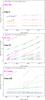 |
Fig. 1 Temporal evolution of knot-core distances for three blazars representative of the three kinematic classes I, II and I/II, selected from the MOJAVE database. |
The presence of non-trivial kinematic behaviours in some sources leads us to clarify some aspects of the classes assignation. Sources with relativistic apparent velocities from their jet base are classified as II, even if they show one or several quasi-stationary knots downstream. The main criterion defining the class II is the ability of producing relativistic knots very close to the core. The sources B2 0202+31, S4 0917+44, 4C +29.45, PKS 1655+077, PHL 5225, CTA 102, 3C 418, PKS 2134+004, 4C +31.63, and also 3C 454.3, as noticed by Jorstad et al. (2013), show this feature. Also, sources with knots close to the core without associated apparent velocities but with relativistic velocities downstream are classified as I/II. The sources Ap Librae, TXS 0730+504, and TXS 2005+403 show this feature.
Some biases can also affect this classification. A lack of monitoring of a source I/II increases the risk of detecting only velocities from quasi-stationary knots, leading to confusion with class I. This effect does not significantly impact the class II sample, as described above; only 10% of this sample presents quasi-stationary components. Finally, all sources close to the discriminating apparent velocity max(βapp) = 2 have a higher risk to be misclassified. To estimate this bias, we count the borderline sources in the interval max(βapp) ∈ [1.5,2.5]. They represent 28% of class I, 3% of class I/II and 4% of class II. This effect is thus potentially significant for class I, which is not surprising because an isotropic repartition of velocities between 0 and 2 c gives 25% of sources in this interval.
2.1. Overlap with spectral classes
A first test of the consistency of this classification is to check its overlap with the standard spectral classes. Blazars are divided in three spectral classes: FSRQs, LBLs/IBLs, and HBLs, which correspond to 125, 23, and 5 sources in our sample, respectively (Table 1). Only sources with well-defined spectral classes are taken into account. The HBL class, which is less luminous in radio, is unfortunately under-represented in the MOJAVE database.
All five blazars referenced as HBLs belong to class I. The IBLs and LBLs belong predominantly to class I/II, but show a significant spread in the other classes. The strong presence of IBLs/LBLs in class I (32%) could be due to the observational bias previously expressed that the less a source is monitored in VLBI, the more chances there are to interpret the source as a class I. The FSRQs are clearly grouped in class II (75%) with a more pronounced spread in class I/II than I, as expected.
This new kinematic classification of blazars proposed here shows a strong link with the standard spectral classification. The discovery of such a link for IBLs and LBLs may provide a valuable key to the understanding of transitions between different classes.
2.2. Overlap with large-scale radio jets
Large-scale, radio-loud AGN morphologies, FR I and FR II, are strongly dependent on extended jets luminosities in radio. Such a link has been highlighted from radio jet samples by Landt et al. (2006) and extended by Kharb et al. (2010). A large number, 118 blazars, of our sample belong to the Kharb sample. This allows us to check the eventual links between VLBI kinematic classes and the large-scale morphologies. The distributions of 1.4 GHz extended radio luminosities of sources and their core/extended jet ratio are plotted in Fig. 2 for the three kinematic classes. As in Kharb et al. (2010), the solid lines indicate FR I-FR II divide with an undifferentiated area FRI/II between (FR II have extended luminosities Lext ≥ 1026 W Hz-1 and FR I Lext ≤ 1024.5 W Hz-1).
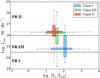 |
Fig. 2 Box plots of extended jets radio luminosities vs. core-extended jet luminosities ratio for the three kinematic classes. Boxes are delimited by the first and last quartiles, middle lines are medians, and dashed lines account for the maximum size of distributions. Horizontal black lines delimit regions where the luminosities of extended jets are typical of FR I or FR II morphologies. |
Overlap of the kinematic classification with spectral classification.
Classes I/II and II are mostly in the FR II domain with strong extended radio luminosities, contrary to class I, which present a median extended luminosity that is almost two orders of magnitude lower than the other classes. This could suggest that large-scale radio jet properties are more affected by the VLBI kinematic difference between class I and the other classes than between classes I/II and II. Their median values, favouring a continuity of extended jet luminosities and extended-core luminosity ratios, are expressed in Table 2.
Knowing that FR II AGN have much more powerful jets than FR I AGN, this trend indicates that the extended jet power follows the VLBI kinematic classification; however, the wide dispersion made this link weak for a source-by-source study. This highlights a potentially different process in jet propagation from the class I sources, which differentiates them from the other populations.
3. Jet physical parameters
Radio VLBI measures, such as apparent velocities, sizes, and luminosities of knots (Lister et al. 2013), allow us to deduce jet physical parameters. Thus, the three kinematical behaviours defined above can be now characterised following physical criteria.
3.1. Doppler factors, Lorentz factors, and angles with the line of sight
Apparent velocities of radio knots are usually associated with the Doppler factor of underlying beam flow (Daly et al. 1996; Jorstad et al. 2005; Onuchukwu & Ubachukwu 2013; Hervet et al. 2015). However, knots of class I sources present quasi-stationary motions that are incompatible with the high Doppler and Lorentz factors suggested by the fast variability of HBLs. We thus only associate apparent velocities and Doppler factors with the sources belonging to classes I/II and II. For each source we assume that the maximum detected apparent velocity is representative of the flow velocity of jets.
Medians of the extended radio jets luminosities (log [W Hz-1]) and of the luminosities ratio core/extended for the three VLBI kinematic classes.
The Doppler factor δ depends on the apparent velocity βapp, but also on the angle θ between the direction of the jet and line of sight, 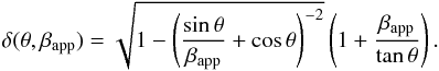 (1)We simulate the radio detection probability on this angle and the maximal measured apparent velocity P(θ,βapp) to define realistic θ angles for the selected sources. For each source, the angle θ is chosen where the probability function is at maximum.
This probability function can be seen as the combination of
-
the intrinsic angle distribution of jets projected on the sky planePproj(θ);
-
the source detection probability depending on the relativistic beaming Pbeam(θ,βapp).
Considering an isotropic distribution of AGN jet directions, their angles to the line-of-sight θ ∈ [θ1,θ2], (θ1<θ2) is proportional to the annulus area of the solid angle described by θ2−θ1. So we can express the distribution Pproj(θn) as ![Mathematical equation: \begin{equation} P_{\rm proj}(\theta_n) \propto \left[\cos \theta_{n-1} - \cos \theta_{n} \right]. \end{equation}](/articles/aa/full_html/2016/08/aa28117-16/aa28117-16-eq42.png) (2)This distribution favours large angles to the line of sight with a maximum at θ = 90°. Hence, if the AGN jets where not relativistic, one should observe many more misaligned radio galaxies than blazars.
(2)This distribution favours large angles to the line of sight with a maximum at θ = 90°. Hence, if the AGN jets where not relativistic, one should observe many more misaligned radio galaxies than blazars.
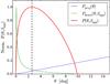 |
Fig. 3 Normalised probability of the jet angle with the line of sight for a given apparent velocity. The probability function shown here is based on the calculated median value of class II sources maximal apparent velocities, namely βapp = 11.6. The angle with a maximal probability, indicated with a dotted line, corresponds to θ = 2.6 deg. |
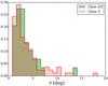 |
Fig. 4 Distribution of the most probable angles θ for classes I/II and II. Areas are normalised. |
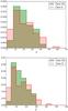 |
Fig. 5 Distribution of the most probable Doppler and Lorentz factors for classes I/II and II. Areas are normalised. |
However, jets are highly relativistic and blazars are strongly beamed, so we have to quantify their overexposure. Knowing that the jet radio flux F comes from synchrotron radiation amplified by Doppler boosting, and that the associated radio spectrum is relatively flat, we have the relation F ∝ δ3. Hence, using the Eq. (1), we can express the source detection probability depending on the relativistic beaming,  (3)With the product of Pproj(θ) and Pbeam(θ,βapp), the general probability can be expressed as a function of a jet direction,
  (4)This probability depends only on the angle to the line of sight, where βapp is an observational constraint. Thus for each source of kinematic classes I/II and II, we can determine the most probable angle of the jet with the line of sight, as shown in Fig. 3.
This method is very effective for knots with high apparent velocities with a well-peaked probability at low angles. This efficiency decreases at low velocities and, because of the weak beaming constraint, the probability tends to the isotropic distribution. The angular distribution of class I/II and II sources deduced from this method is represented in Fig. 4.
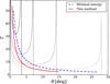 |
Fig. 6 Lorentz factor and jet angle for various values of apparent velocities βapp ∈ [2;50]. We compare results from our method developed here and the minimal energy method. Greyscale lines represent the Lorentz factor values following jet angles for a sample of given apparent velocities (lower to upper lines: 2 c, 4 c, 8 c, 16 c, and 32 c). |
We can deduce the Doppler factor distribution from this angular distribution via Eq. (1). Similarly, we also deduce the Lorentz factor distribution via the equation 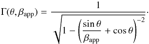 (5)Doppler and Lorentz factors distributions are shown in Fig. 5, which shows that the distribution peaks of class I/II and II coincide, suggesting similar launching processes of the flow. Class II presents slightly wider distributions than those of class I/II.
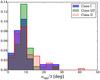 |
Fig. 7 Inner jet half opening angles distribution for classes I, I/II et II. Areas are normalised. |
Our method can be compared to the method that minimises the intrinsic kinetic power of the jet. From the principle of least action, we can assume that the observation angle is close to the observation angle that minimises the Lorentz factor value for a given apparent velocity. We present in Fig. 6 the Lorentz factor values for the “minimal energy” and our method. In any case the Lorentz factor found in our method remains close to the lowest possible value, which reinforces the relevance of our statistical approach. All of the observation angles, Doppler and Lorentz factor deduced in this section are reported in Table A.1.
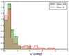 |
Fig. 8 Intrinsic half opening angles distribution for classes I/II et II. Areas are normalised. |
3.2. Inner jets aperture angles
In Hervet et al. (2015), we showed that the radio knots of the blazar AP Librae increases linearly with the radio core distance. This allowed us to define an aperture angle of the inner jet. Now we apply this method for the blazars of our three classes to understand whether these aperture angles are dependent on the knot kinematics.
The radio knot flux distributions on the sky plane are fitted by 2D symmetrical Gaussians (Lister et al. 2013), thus we can estimate the apparent half aperture angles by making a linear regression of their half full-width at half-maximum (FWHM) following their distances to the radio core. This method was already used in Jorstad et al. (2005) and Hervet et al. (2015).
Sources with a correlation coefficient of the linear regression, R2 > 0.1, are selected in our sample, and only three sources do not pass this selection; thus, this gives us very strong confidence in the conical description of blazar jets. The apparent angles distribution deduced from this method is shown for each class in Fig. 7, and reported source by source in Table A.1.
Knowing the apparent aperture angle αapp and the jet angle to the line-of-sight θ, calculated in Sect. 3.1, we can deduce the intrinsic aperture angle of the inner jet α = αappsin(θ). Having no strong constraints on the θ angle for class I sources, we present these intrinsic angles for classes I/II and II only. The distribution of α angles is shown in Fig. 8 and the values are given in Table A.1.
3.3. Radio knot evolution
In previous sections we showed that classes I/II and II do not present any significant differences in terms of jet angles with the line of sight, Doppler factors, Lorentz factors, or inner jet aperture angles. Thus, the kinematical differences between these classes cannot be strongly linked with any of these parameters.
It is also possible to study the knot evolution for the three classes with the radio knot features given in Lister et al. (2013), such as radio flux and Gaussian FWHM, which we can link to their sizes. The knot-core distance evolution is not used in this study because of its strong dependence on the observation angles, poorly constrained in class I sources. Hence, we determine the flux and size median evolutions, dFk/dt and dDk/dt, for each source, respectively. Their importance is balanced by their visibility time in radio to avoid an over-representation of some knots. Of course, only knots identified during multiple observations are taken into account.
Figure 9 shows a clear distinction between the three kinematic classes. The median values of class I sources show an almost non-evolution of their knots, regarding their flux or size. The other classes show a clear expansion and cooling with values increasing continuously between class I/II and II. Median values of size and flux evolutions are referenced in Table 3, quantifying the continuity between dominant regimes for the three classes.
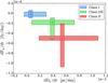 |
Fig. 9 Box plots of knot diameter evolution vs. knot flux evolution for sources of the three kinematic classes. Boxes are delimited by the first and last quartiles; middle lines are medians. |
This confirms that knots with quasi-stationary motion at the jet base also have a quasi-stationary evolution without cooling nor expansion contrary to knots expelled in jets of classes I/II and II, which mainly follow an adiabatic expansion. This implies that knots of class I sources have a stable energy tank over long periods. The description of these knots as structural stable stationary shocks in jets powered by a continuous underlying flow, as developed in the following sections, happens to be the most likely explanation of this phenomenon.
4. Study of an intermediate blazar, the BL Lac case
The hybrid kinematics of class I/II VLBI jets is very surprising. Intuitively one would expect a smooth kinematical transition between classes I and II with knots at intermediate velocities, but this is not the case and Lorentz factor values of class I/II, which were deduced in Sect. 3.1, are not significantly different from those of class II. This hybrid behaviour with quasi-stationary knots near the base and relativistic knots downstream seems to give a valuable clue regarding the intrinsic nature of these zones.
To further study these objects, we now focus on the blazar BL Lac itself, which is the most studied blazar of the intermediate class, and presents one of the best radio VLBI monitoring over numerous years.
Median values of the size and flux evolution of radio knots for the three classes, illustrating a continuity between VLBI jet behaviours.
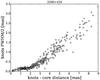 |
Fig. 10 Half FWHMs of BL Lac radio knots following their apparent distance to the radio core. A clear change of the opening angle happens around 2 mas from the core. Adapted from data published in Lister et al. (2013). |
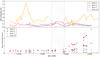 |
Fig. 11 Evolution of flux and size of four radio knots of BL Lac 5,6,7 and 10. The grey hatching area represents the duration of the perturbation propagation in the VLBI jet from the knot 10 to the knot 5 between the October 14th 2001 and the July 7th 2002. The non-observation of the knot 7 and the appearance of the knot 10 during the perturbation propagation is a sign of an abrupt evolution of the same knot. |
In Fig. 10 we notice a strong increase of the inner jet aperture angle for the apparent core distance Lapp,jet = 2 mas. By linear approximation, we deduce two apparent aperture angles αapp,1/ 2 = 4.6° and αapp,2/ 2 = 21.5° upstream and downstream 2 mas.
4.1. Transient knots and propagation of a perturbation
Some of the apparent motions of BL Lac radio knots present a quick evolution. Indeed, some long-term quasi-stationary knots are quickly accelerated to relativistic velocities, as shown in Fig. 12. We call these “transient knots” because they exhibit a transition between knots of class I and those of the class II.
Figure 12 shows that three knots (5,6 and 10) are accelerated in a short time around the beginning of 2002. This suggests that the internal jet undergoes a perturbation on several parsecs during few months in the observer frame. We estimate a temporal gap of 266 days between the ejection of knot 10 at the base of the jet on October 14, 2001 and the acceleration of knot 6 at 2.6 mas from the core around July 7, 2002. The apparent velocity of such a propagation would be βapp,P = 14.9, which is significantly higher than the highest apparent velocity measured in VLBI at 9.95 c.
The propagation velocity of a perturbation could be a more reliable indicator of the intrinsic flow velocity than the knot motions. Indeed the radio knots are supposed to have particle density that is higher than the underlying flow. Admitting that this flow carries the knots along, the radio knot velocities should systematically underestimate the flow velocity. As presented in Sect. 2, the fastest radio knot is chosen to minimise this bias.
This effect can be balanced, however, especially for class II sources. In these jets, radio knots have relativistic velocities from the radio core and propagate over large distances, and we can thus assume that they reach a kinetic equilibrium with the underlying flow more quickly and, thereby, are more effective velocity markers. With this direct indicator of the intrinsic flow velocity in the blazar BL Lac, we can constrain various physical parameters, as developed in Sect. 3.1 (see Table 4).
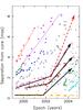 |
Fig. 12 Knot distances to the radio core of BL Lac over 7 yr, adapted from Lister et al. (2013). Knots 5 and 6 are identified as transients; knot 10 seems ejected from the closest stationary zone from the core. The dashed red arrow represents the displacement of a probable perturbation along the jet having modified the kinematics of knots. |
Physical parameters of BL Lac deduced from the fast propagation of a perturbation in the jet.
4.2. Transient knot evolution
The effects of the perturbation described above on the knot evolution is now studied. The intrinsic properties of radio knots can be defined by two observables, size and flux evolution; these are presented in Fig. 11.
We notice that knot 10 shows a high flux when detected and then decreases quickly. During its ejection (0.513 mJy and 0.14 mas, respectively), the flux and size of knot 10 are relatively close to those of the stationary knot 7 just before (0.681 mJy and 0.12 mas). Also, knot 7 is no longer detected during the four following observations between August 6, 2001 and June 15, 2002. Thus, all these evidences suggest that knot 10 is nothing else than knot 7 ejected from its stationary zone accompanied by a strong decrease in flux. The effect of this perturbation on knots 5 and 6 farther from the core is less obvious with a slight increase and decrease of their flux during the interval estimated for the propagation of this perturbation.
One can also see in Fig. 11 that the three knots (5, 6, and 10) are in expansion regime after the perturbation passage. This is consistent with their motion observed in the jet. Knot 5 shows a faster expansion in accordance with the increase of the inner jet opening angle after 2 mas (see Fig. 10). The reobservation of stationary knot 7 after the perturbation indicates that this unstable zone is naturally reforming, highlighting an intrinsic structure of the jet, which we develop in the following section.
5. Discussion and interpretation
We propose here a qualitative scenario that is able to take the various radio knot characteristics discussed above into account. Observed apparent velocities, variabilities, and also multi-wavelength modellings prove that AGN jets host strong flows with relativistic velocities. As these velocities are usually much higher than the Alfven velocity, it is very likely to have the formation of recollimation shocks. Such shocks are commonly invoked for the radio core description (Marscher & Gear 1985) or for some stationary knots as HST1 in M 87 (Bromberg & Levinson 2009) and knot 7 of BL Lac (C7 in Cohen et al. 2014). These scenarios are based on the presence of one powerful recollimation shock that is able to change the jet structure; this is usually known as the master recollimation shock (MRS). The stationary knot string structure present in class I and I/II sources, as defined in this paper, provides evidence about the possible presence of multiple recollimation shocks in jets. These multi-shocks structures are also predicted by relativistic MHD simulations. For example, Mizuno et al. (2015) recently highlighted the impact of magnetic field topologies on the efficiency of recollimation shock on particle acceleration. These authors show that a longitudinal magnetic field induces more powerful recollimation shocks than any other magnetic topology. Otherwise, magnetic field topologies deduced from the Faraday rotation in radio jets by Kharb et al. (2008a,b) and confirmed by Gabuzda et al. (2014) indicate that HBLs are dominated by a longitudinal field. In contrast, LBLs and FSRQs present a two-component structure with an inner jet that is dominated by a toroidal field included in a wider external jet that is dominated by a longitudinal field.
These various observed magnetic topologies support the scenario of multiple recollimation shocks. Dominant longitudinal fields observed in HBLs are more able to effectively accelerate particles in shocks, and multiple shock structures, as in class I sources, can further increase the particle acceleration (Meli & Biermann 2013). The VHE properties of HBLs suggest that these objects are, by nature, the most efficient particle accelerators of all of the blazars, which is consistent with that scheme. Thus, the synchrotron peak frequency appears to be linked to the shock efficiency, depending on the jet magnetic topologies.
We focus now on various kinematics of radio knots. A key point in differentiating blazars is the jet power. It is recognised that spectral classes are a function of the jet power, that is PFSRQ>PLBL/IBL>PHBL (Meyer et al. 2011; Celotti & Ghisellini 2008). However, these powers alone do not explain why some knots are stationary while others are not. The kinematic classification presented in this paper supports an interpretation as described below. We give a schematic view of this scheme in Fig. 13. This scheme does not intend to describe the complexity of each individual source of this study, but summarises the dominating behaviour of the three blazar populations considered for this classification.
-
Kinematic class I: the presence of stable recollimation shocks in class I sources, as shown in Sect. 3.3, suggests that the longitudinal magnetic field plays a more important role than in other sources. A strong magnetic compression induced by a longitudinal field associated with a low kinetic power maintains a stable structure along the jet up to the magnetic field dissipation after successive shocks, in which particle acceleration occurs at the expense of the magnetic energy. In accordance to this interpretation, HBL sources that belong to class I are known to be closer to the equipartition than FSRQs with a more significant magnetic field. Also, the peculiar large-scale low luminosity of class I, shown in Fig. 2, is in agreement with this peculiar magnetic topology, which should induce a strong dissipation of energy before the large scales.
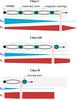
Fig. 13 Scheme of the three kinematic classes I, I/II, and II. We suppose that the various kinematics come from various balances between the internal jet magnetic energy, Em, and the kinetic energy, Ec. The width of these components is representative to their relative strength along the jets.
-
•
Kinematic class II: associated with class II, FSRQs have jets that are widely dominated by particle kinetic energy and do not allow the existence of a successive standing shock structure. Recollimation shocks can be generated at the jet base, where the magnetic field is the most powerful, but seems highly unstable and systematically carried downstream by the underlying flow. As these shock zones are no longer magnetically constrained, they follow an adiabatic expansion along jets, as shown in Sect. 3.3.
-
•
Intermediate kinematic class I/II: intermediate sources are very interesting because they have stationary knots at the jet base and relativistic velocities detected downstream. We assume that the magnetic energy is sufficient near the jet base to maintain a stationary shock structure. This energy is however dissipated in each shock into radiative and kinetic energy. From a certain distance to the core, the magnetic structure becomes unstable and shocks are finally carried out in the same way as those of class II before they are naturally reformed, since they depend on the internal structure and power equilibrium of jets.
Another aspect to take into account is that sources of classes I/II and II are more likely to have an imbricated jet structure. This structure generates instabilities because the shearing is able to break the recollimation shock strings of the internal jet, but maintain a good general collimation because of its strong kinetical power (Meliani & Keppens 2007, 2009).
This general interpretation, which is consistent with the observations, brings the idea that blazars jets are not described by one powerful recollimation shock alone, but the number and kinematics of these recollimation shocks depends on the energetic balances of jets. Furthermore, a newly published paper from Gómez et al. (2016), regarding the ultra high resolution of the BL Lac jet, reports on the detection of two other stationary knots that are closer to the core than knot 7 described above; these authors associate these knots with several recollimation shocks. This study reinforces our proposed scenario describing class I/II.
6. Conclusion
The usual blazar classification based on the SED shape informs the microphysics of a small portion at high energy of the total particle population of jets. Conversely, the new kinematical classification proposed in this paper, provides macrophysics information about the structure and propagation of jets. Because the VLBI resolution is able to access projected sizes at the submilliarcsecond scale, we can reach the regions closest to those responsible for high energy emissions.
The link that we found between spectral and kinematic classifications (class I corresponding to HBLs, class I/II corresponding to IBLs and LBLs, and class II corresponding to FSRQs) gives valuable clues to the area and mechanisms responsible for the particle acceleration. A scenario of multiple recollimation shocks is favoured to interpret this link and also to describe the various behaviours of VLBI jets. We highlight some long-standing issues of AGN classification, which are naturally explained within such a scenario:
It can resolve the apparent Lorentz factor paradox between jets showing evidence for high Lorentz factor values and quasi-stationary VLBI knots.
It account for the singular VLBI behaviour of intermediate sources classified as I/II.
It can chart the destructuration and restructuration of a knotty VLBI structure after a strong flare, as observed in BL Lac.
It provides a consistent scheme linking magnetic topology, synchrotron peak frequency, and jet VLBI kinematics.
Possible biases that can affect the significance of the results are the lack of detailed VLBI monitoring of certain sources that can lead to uncertainties about the detected velocities of the knots. It was shown, however, that these effects are only potentially significant for class I. Thus, the global scenario presented here is not jeopardised.
In any case this scenario with multiple recollimation shocks in blazars will be tested along several paths. The MHD modelling aspect will be deepened to test the viability of shocks and to find out, in particular, if we can reasonably reproduce the behaviour of class I/II sources. Class I knots are associated with multiple stationary shocks. This gives constraintson their sizes and inter-shocks distances, which can be checked by VLBI studies. Still, in class I sources, one would expect that perturbations propagate in their jets without destructuring them, passing through shocks by increasing their luminosities. Variability measures that are consistent with the time delay between shocks could also efficiently test this scenario.
Monitoring Of Jets in Active galactic nuclei with VLBA Experiments, http://www.physics.purdue.edu/MOJAVE/
Acknowledgments
This research has made use of data from the MOJAVE database that is maintained by the MOJAVE team (Lister et al. 2009).
References
- Bromberg, O., & Levinson, A. 2009, ApJ, 699, 1274 [NASA ADS] [CrossRef] [Google Scholar]
- Celotti, A., & Ghisellini, G. 2008, MNRAS, 385, 283 [NASA ADS] [CrossRef] [Google Scholar]
- Cohen, M. H., Meier, D. L., Arshakian, T. G., et al. 2014, ApJ, 787, 151 [NASA ADS] [CrossRef] [Google Scholar]
- Daly, R. A., Guerra, E. J., & Guijosa, A. 1996, in Energy Transport in Radio Galaxies and Quasars, eds. P. E. Hardee, A. H. Bridle, & J. A. Zensus, ASP Conf. Ser., 100, 73 [Google Scholar]
- Gabuzda, D. C., Reichstein, A. R., & O’Neill, E. L. 2014, MNRAS, 444, 172 [NASA ADS] [CrossRef] [Google Scholar]
- Georganopoulos, M., & Kazanas, D. 2003, ApJ, 594, L27 [NASA ADS] [CrossRef] [Google Scholar]
- Giroletti, M., Hada, K., Giovannini, G., et al. 2012, A&A, 538, L10 [NASA ADS] [CrossRef] [EDP Sciences] [Google Scholar]
- Gómez, J. L., Lobanov, A. P., Bruni, G., et al. 2016, ApJ, 817, 96 [NASA ADS] [CrossRef] [Google Scholar]
- Hervet, O., Boisson, C., & Sol, H. 2015, A&A, 578, A69 [NASA ADS] [CrossRef] [EDP Sciences] [Google Scholar]
- Hovatta, T., Valtaoja, E., Tornikoski, M., & Lähteenmäki, A. 2009, A&A, 494, 527 [NASA ADS] [CrossRef] [EDP Sciences] [Google Scholar]
- Jorstad, S. G., Marscher, A. P., Lister, M. L., et al. 2005, AJ, 130, 1418 [NASA ADS] [CrossRef] [Google Scholar]
- Jorstad, S. G., Marscher, A. P., Smith, P. S., et al. 2013, ApJ, 773, 147 [NASA ADS] [CrossRef] [Google Scholar]
- Kharb, P., Gabuzda, D., & Shastri, P. 2008a, MNRAS, 384, 230 [NASA ADS] [CrossRef] [Google Scholar]
- Kharb, P., Lister, M. L., & Shastri, P. 2008b, Int. J. Mod. Phys. D, 17, 1545 [NASA ADS] [CrossRef] [Google Scholar]
- Kharb, P., Lister, M. L., & Cooper, N. J. 2010, ApJ, 710, 764 [NASA ADS] [CrossRef] [Google Scholar]
- Kovalev, Y. Y., Lister, M. L., Homan, D. C., & Kellermann, K. I. 2007, ApJ, 668, L27 [NASA ADS] [CrossRef] [Google Scholar]
- Lähteenmäki, A., & Valtaoja, E. 1999, ApJ, 521, 493 [NASA ADS] [CrossRef] [Google Scholar]
- Landt, H., Perlman, E. S., & Padovani, P. 2006, ApJ, 637, 183 [NASA ADS] [CrossRef] [Google Scholar]
- Lister, M. L., Cohen, M. H., Homan, D. C., et al. 2009, AJ, 138, 1874 [NASA ADS] [CrossRef] [Google Scholar]
- Lister, M. L., Aller, M. F., Aller, H. D., et al. 2013, AJ, 146, 120 [NASA ADS] [CrossRef] [Google Scholar]
- Marscher, A. P., & Gear, W. K. 1985, ApJ, 298, 114 [NASA ADS] [CrossRef] [Google Scholar]
- Meier, D. L. 2013, in Eur. Phys. J. Web Conf., 61, 1001 [Google Scholar]
- Meli, A., & Biermann, P. L. 2013, A&A, 556, A88 [NASA ADS] [CrossRef] [EDP Sciences] [Google Scholar]
- Meliani, Z., & Keppens, R. 2007, A&A, 475, 785 [NASA ADS] [CrossRef] [EDP Sciences] [Google Scholar]
- Meliani, Z., & Keppens, R. 2009, ApJ, 705, 1594 [NASA ADS] [CrossRef] [Google Scholar]
- Meyer, E. T., Fossati, G., Georganopoulos, M., & Lister, M. L. 2011, ApJ, 740, 98 [NASA ADS] [CrossRef] [Google Scholar]
- Mizuno, Y., Gómez, J. L., Nishikawa, K.-I., et al. 2015, ApJ, 809, 38 [NASA ADS] [CrossRef] [Google Scholar]
- Onuchukwu, C. C., & Ubachukwu, A. A. 2013, Ap&SS, 348, 193 [NASA ADS] [CrossRef] [Google Scholar]
- Piner, B. G., & Edwards, P. G. 2004, ApJ, 600, 115 [NASA ADS] [CrossRef] [Google Scholar]
Appendix A: Additional table
Kinematic classification and physical parameters of our source sample.
All Tables
Medians of the extended radio jets luminosities (log [W Hz-1]) and of the luminosities ratio core/extended for the three VLBI kinematic classes.
Median values of the size and flux evolution of radio knots for the three classes, illustrating a continuity between VLBI jet behaviours.
Physical parameters of BL Lac deduced from the fast propagation of a perturbation in the jet.
All Figures
|
Fig. 1 Temporal evolution of knot-core distances for three blazars representative of the three kinematic classes I, II and I/II, selected from the MOJAVE database. |
| In the text | |
|
Fig. 2 Box plots of extended jets radio luminosities vs. core-extended jet luminosities ratio for the three kinematic classes. Boxes are delimited by the first and last quartiles, middle lines are medians, and dashed lines account for the maximum size of distributions. Horizontal black lines delimit regions where the luminosities of extended jets are typical of FR I or FR II morphologies. |
| In the text | |
|
Fig. 3 Normalised probability of the jet angle with the line of sight for a given apparent velocity. The probability function shown here is based on the calculated median value of class II sources maximal apparent velocities, namely βapp = 11.6. The angle with a maximal probability, indicated with a dotted line, corresponds to θ = 2.6 deg. |
| In the text | |
|
Fig. 4 Distribution of the most probable angles θ for classes I/II and II. Areas are normalised. |
| In the text | |
|
Fig. 5 Distribution of the most probable Doppler and Lorentz factors for classes I/II and II. Areas are normalised. |
| In the text | |
|
Fig. 6 Lorentz factor and jet angle for various values of apparent velocities βapp ∈ [2;50]. We compare results from our method developed here and the minimal energy method. Greyscale lines represent the Lorentz factor values following jet angles for a sample of given apparent velocities (lower to upper lines: 2 c, 4 c, 8 c, 16 c, and 32 c). |
| In the text | |
|
Fig. 7 Inner jet half opening angles distribution for classes I, I/II et II. Areas are normalised. |
| In the text | |
|
Fig. 8 Intrinsic half opening angles distribution for classes I/II et II. Areas are normalised. |
| In the text | |
|
Fig. 9 Box plots of knot diameter evolution vs. knot flux evolution for sources of the three kinematic classes. Boxes are delimited by the first and last quartiles; middle lines are medians. |
| In the text | |
|
Fig. 10 Half FWHMs of BL Lac radio knots following their apparent distance to the radio core. A clear change of the opening angle happens around 2 mas from the core. Adapted from data published in Lister et al. (2013). |
| In the text | |
|
Fig. 11 Evolution of flux and size of four radio knots of BL Lac 5,6,7 and 10. The grey hatching area represents the duration of the perturbation propagation in the VLBI jet from the knot 10 to the knot 5 between the October 14th 2001 and the July 7th 2002. The non-observation of the knot 7 and the appearance of the knot 10 during the perturbation propagation is a sign of an abrupt evolution of the same knot. |
| In the text | |
|
Fig. 12 Knot distances to the radio core of BL Lac over 7 yr, adapted from Lister et al. (2013). Knots 5 and 6 are identified as transients; knot 10 seems ejected from the closest stationary zone from the core. The dashed red arrow represents the displacement of a probable perturbation along the jet having modified the kinematics of knots. |
| In the text | |
|
Fig. 13 Scheme of the three kinematic classes I, I/II, and II. We suppose that the various kinematics come from various balances between the internal jet magnetic energy, Em, and the kinetic energy, Ec. The width of these components is representative to their relative strength along the jets. |
| In the text | |
Current usage metrics show cumulative count of Article Views (full-text article views including HTML views, PDF and ePub downloads, according to the available data) and Abstracts Views on Vision4Press platform.
Data correspond to usage on the plateform after 2015. The current usage metrics is available 48-96 hours after online publication and is updated daily on week days.
Initial download of the metrics may take a while.